I. INTRODUCTION

B i n d Source Separation (BSS) is a high-level image/sign processing mechanism with numerous applications including sound signals, communication, images, and biomedicine [1,2,3,4]. The goal of BSS is to recover the source (signals/images) from a noisy source with little known information. Non-Gaussianity [5,6], mutual information minimization [7,8], maximum likelihood [9], and neural networks [10,11,12] are some of the BSS algorithms that have been debated from various perspectives. Denoising and optimization procedures are critical in BSS. The noise separation step determines the separability of the noise, and the optimization step determines the best solution for the objective function obtained from the denoising algorithm. Because of the variable features of generalized distributions, they generally produce good blind denoising results.

In the Independent Component Analysis (ICA) framework, precisely estimating the statistical model of the sources remains an open and difficult problem [2]. Practical BSS procedures make use of difficult, complicated source distributions, as well as situations involving abundant sources with varying mixed probability density functions (pdf). Numerous parametric density models have been made available in recent literature in this direction. Similar models include the generalized gamma density [13], the generalized Alfa-Beta distribution (AB-divergences) [14], and combinations and generalizations such as the super and generalized Gaussian admixture model [15], the generalized Gaussian density [16], the Pearson family of distributions [17], and the so-called extended generalized lambda distribution [18], which is an extended parameterization of the previously mentioned generalized lambda distribution and generalized beta distribution models [19].

We can find out how medical signals studies are very important and many researches are published continuously, for instants, Stationary wavelet transform based Electrocardiogram (ECG) signal denoising method [20], Electrocardiogram signal denoising [21], semi-supervised deep blind compressed sensing for analysis and reconstruction of biomedical signals from compressive measurements [22], biomedical signals reconstruction and zero-watermarking using separable fractional order Charlier-Krawtchouk transformation and sine cosine algorithm [23], research on AR-AKF model denoising of the Electromyography (EMG) signal [24], threshold parameters selection for empirical mode decomposition-based EMG signal denoising[25], Variational Mode Decomposition (VMD)-based denoising methods for surface electromyography signals [26], ECG signal denoising method using conditional generative adversarial net [27], motion artifacts suppression from Electromyogram (EEG) signals using an adaptive signal denoising method [28], research on improved Flexible Analysis Wavelet Transform (FAWT) signal denoising method in evaluation of firefighter training efficacy based on sEMG [29], lung sound signal denoising using discrete wavelet transform and artificial neural network [30], deep learning-based framework For ECG signal denoising [31], denoising of ECG signals using weighted stationary wavelet total variation [32], denoising of medical images utilizing neural network [33], denoising of biomedical images using two-dimensional Fourier-Bessel series [34].

Although Fast ICA has drawbacks, such as the difficulty of optimizing the log-likelihood function, which means the suitable source signals aren't insulated, and the order of the independent components (ICs) is difficult to determine, it is still one of the most robust methods and generally drives veritably good results.

In addition, we present Sparse Code Shrinkage [35], a statistically principled method. which is very similar to independent component analysis.

Still, studying medical signals has become extremely important and necessary; it is extremely difficult to extract useful information from these signals in the time domain simply by observing them. They are fundamentally non-linear and non-stationary. Biomedical signals are generally affected by various types of noise, which is considered a difficult and difficult problem. For example, one of the challenges of EEG technology is that the electrical activity generated by the brain is minute, on the order of a millionth of a volt. As a result, scalp recorded electrical pulses are a mixture of genuine brain signals mixed with a lot of noise-called artifact-generated by other parts of the body, such as heart activity, eye movements and blinks, other facial muscle movements, and so on, which produce electrical signals 100 times greater than those produced by the brain. Furthermore, the background noise is typically generated outside of the brain.

As a result, in order to extract the important information from the signals, noise must be removed. Many different advanced signal processing mechanisms have been developed to accomplish this. The Fractional Weibull Distribution (FWD) with ICA is presented in this paper for noise removal from biomedical signals. The accuracy of the proposed algorithm is measured, and the numerical results show that the FWD consistently produces good results. The remainder of the paper is structured as follows: Section 2 introduces the BSS model. The FWD is discussed in Section 3. In Section 4, we estimate the parameters of FWD using maximum likelihood. Finally, we demonstrate the computational efficiency of our proposed mechanism.

II. BLIND SOURCE SEPARATION (BSS) MODEL

denotes an independent source signal vector that comes from N signal sources, then we can get the observed mixtures

$\mathbf{X}(\mathfrak{t})=[{\mathbf{x}}_1(\mathfrak{t}),{\mathbf{x}}_2(\mathfrak{t}),\dots ,{\mathbf{x}}_{\mathrm{K}}(\mathfrak{t}){]}^{\mathrm{T}}(\mathbf{N}=\mathbf{K})$ under the circumstances of the instantaneous linear mixture. This leads us to the BSS model

where $A$ is a $N\times N$ mixing matrix. The target of the BSS algorithm is to recover the sources from mixtures $x(t)$ by using

where $\mathbf{W}$ is a $\mathbf{N}\times \mathbf{N}$ separation matrix and $\mathbf{U}(t)=[{\mathbf{u}}_1(t),{\mathbf{u}}_2(t),\dots ,{\mathbf{u}}_N(t){]}^{\mathrm{T}}$ is the estimate of $\mathbf{N}$ sources.

Generally, sources are assumed to be unit-variance and zero-mean signals with at most one of Gaussian distribution. To solve the source estimation problem, the unmixing matrix $W$ must be obtained. Generally, the maturity of BSS approaches performs ICA, by basically optimizing the negative log-likelihood (objective) function concerning the un-mixing matrix $W$ such that:

where $\mathrm{E}[\cdot ]$ represents the expectation operator and ${\mathbf{p}}_{\mathbf{u}\mathbf{1}}({\mathbf{u}}_1)$ is the model for the marginal pdf of ${\mathbf{u}}_1$, for all $l=1,2,\dots ,N$. In effect, when the distribution of the sources is correctly assumed, the maximum likelihood (ML) principle leads to estimating functions, which are the source score functions [15]

In principle, the separation criterion can be optimized by any suitable ICA algorithm where contrasts are employed (see; e.g., [2]). The FastICA [3], based on

where, as defined in [4]

where $\phi (t)=[{\phi }_1(u_1),{\phi }_2(u_2),\dots ,{\phi }_n(u_n){]}^{\mathrm{T}}$, valid for all $l=1,2,\dots ,n$.

The following section explains FWD for signal modelling.

III. INDEPENDENT COMPONENT ANALYSIS (ICA)

a) Definition of ICA

"It's a technique for identifying underlying factors or components in multivariate (multi-dimensional) statistical data." The ICA differs from other methods in that it seeks components that are both statistically independent and non-Gaussian." [36]

Now, assume that we observe $n$ linear mixtures $x_1,\dots ,x_n$ of $n$ independent components [37].

The time indicator $t$ has been removed; in the ICA model [36,37], it is assumed that each admixture $x_i$ and independent element $s_k$ is an arbitrary variable rather than a suitable time signal. The observed values $x_j(t)$, for example, microphone signals, are a sample of this arbitrary variable. As a preliminary step, we can assume that both the admixture variables and the independent factors have zeremean. If not, the observed variables, $x_i$ can always be centered by reducing the sample mean, resulting in a zero-mean model. It would be possible to use a vector-matrix memo instead of totalities as in the previous equation. Let's denote by $x$ the arbitrary vector whose rudiments are the fusions $x_1,\dots ,x_n$, and by $s$ the arbitrary vector with rudiments $s_1,\dots ,s_n$, and by A the matrix with rudiments $a_{ij}$. The mixing model is written as

Also, can be written as

The statistical model in Eq. 6 is called the ICA model.

It's a generative model that describes how the observed data are generated by a process of mixing the factorssi

The main idea for ICA is veritably simple, assume that the components $si$ are statistically independent. also, they must have non-Gaussian distributions.

b) The Fast ICA Algorithm

We introduced various non-Gaussianity measures [36,37], i.e. objective functions for ICA estimation. In practice, we also require an algorithm for maximizing the cost function. The FastICA Algorithm is one of the most effective ICA algorithms, and it will be used in our new proposed system.

c) Sparse Code Shrinkage

Another example of using the ICA decomposition to find ICA filters for medical (images/signals), removing noise from images (signals) contaminated with Gaussian noise. A collection of medical images was used. As $x$, represent the vector of pixel grey levels of a window in an image. The elements of $x$ are indexed by their position in the image window or patch. The 2-D structure of the windows is irrelevant here:

Row-by-row scanning was used to convert a square image window into a vector.

Now, suppose the noisy image model:

where $nn$ is uncorrelated noise, with elements similarly indexed in the image window as $xx$, and $zz$ is the measured image window contaminated with noise. Assuming that $nn$ is Gaussian and $xx$ is non-Gaussian.

There are numerous methods for removing noise, including Discrete Fourier Transform (DFT) transformation to spatial frequency space, low-pass filtering, and return to image space via Inverse Discrete Fourier Transform (IDFT) [38]. However, this is inefficient. Better methods include the recently introduced Wavelet Shrinkage method [39], which employs a wavelet-based transform, or methods based on median filtering [38]. These methods, however, did not take advantage of image statistics.

We present Sparse Code Shrinkage [35], another statistically principled method that is very similar to independent component analysis. Compactly, if we form the density of $\mathbf{x}$ by ICA, and suppose $\mathbf{n}$ Gaussian, the Maximum Likelihood (ML) solution for $\mathbf{x}$ given the measurement $\mathbf{z}$ can be developed in the signal model (10).

The ML solution can be computed simply, albeit roughly, by using an orthogonalized version of ICA decomposition. The transform can then be given by

where $W$ is an orthogonal matrix which is the best orthogonal approximation of the inverse of the ICA mixing matrix. The noise term $Wn$ is still Gaussian and white. With a quietly suitable choice of orthogonal transform, however, the density of $Wx=s$ becomes largely non-Gaussian, e.g., super-Gaussian with a highly positive kurtosis. This relies obviously on the original $x$ signals, as assuming, in fact, there exists a model $x=W^{T}s$ for the signal, where the "source signals" or elements of $s$ have a positive kurtotic density, in such case the ICA transform gives highly super-Gaussian components.

It was shown in [35] that, assuming a Laplacian density for $s_i$, the ML solution for $s_i$ is given by a "shrinkage function" ${\hat{s}}_i=g([Wz{]}_i)$, or in vector form, $\hat{\mathbf{s}}=g(\mathbf{W}\mathbf{z})$. Function $g(.)$ has a characteristic shape: it is zero close to the origin and then linear after a cutting value depending on the parameters of the Laplacian density and the Gaussian noise density. Supposing other forms for the densities, other optimal shrinkage functions can be obtained [35].

The shrinkage process in the Sparse Code Shrinkage model is performed in the rotated space, and the signal estimation in the original space is obtained by rotating back:

Thus, we obtain the Maximum Likelihood estimation for the image window $\mathbf{x}$ in which most of the noise has been removed. The rotation operator $\mathbf{W}$ is such that the sparsity of the components $\mathbf{s}=\mathbf{W}\mathbf{x}$ is maximized. The operator can be learned with a modification of the FastICA algorithm; see [35] for details. The results of the Sparse Code Shrinkage method and classic wiener filtering are given, indicating that Sparse Code Shrinkage may be a promising approach. The noise is reduced without blurring edges or other sharp features as much as in wiener filtering. This is largely due to the strongly nonlinear nature of the shrinkage operator, which is optimally adapted to the inherent statistics of images.

IV. PROPOSED ALGORITHM

a) Fractional Weibull distribution

Fractional Weibull Distribution (FWD) or the fractional Weibull probability density (FWPD).

where is the shape parameter and is the scale parameter of the Weibull distribution. Compared to the

Hence, the log-likelihood function $\mathcal{L}=\log \ell$ becomes

Therefore, the maximum likelihood estimation of $\lambda$ and $k$ is derived from the derivatives of $\mathcal{L}$. They should satisfy the following equations:

The system of equations (20, 21) must be solved in order to estimate the value of parameters. However, it can be solved using MATLAB or using the Newton-Raphson method as in [19,37]. also, the genetic algorithm (GA) [40,41] can be used as an alternative numerical method to estimate the parameters the GA standard Weibull distribution, equation (13) has a scaling factor (1- $\delta 1$ ) that is smaller than 1.0, which is the reason why equation (13) is called the fractional Weibull distribution, or the fractional Weibull probability density (FWPD).

The corresponding cumulative distribution is given by:

b) Maximum likelihood estimation method

To demonstrate the method, the Maximum Likelihood Estimation (MLE) procedure is used to determine the values of the Weibull parameters, $\lambda$ and $k$, to illustrate the method. For this purpose, the first-order optimality conditions below are used.

c) Parameter stimulation

To estimate the parameters of FWD, the maximum likelihood is used. Let ${\mathbf{X}}_1,{\mathbf{X}}_2,\dots ,{\mathbf{X}}_n$ be a sample of size $N$ from an FWD. Then the log-likelihood function $(\mathcal{L})$ is given by:

V. NUMERICAL RESULTS

Numerical experiments show that the estimated parameters provide an acceptable solution with significantly fewer function evaluations; we generate random samples from the fractional Weibull distribution along with various parameter combinations, and then the ML estimates are obtained.

A procedure called (ga) in MATLAB can be used to obtain the ML estimate, and a similar procedure is extremely fast and accurate. The proposed mechanism produces outstanding results for both EEG and electrocardiogram (ECG) signals.

VI. EXPERIMENTAL RESULTS

Resolve FastICA algorithm for (BSS). It is based on the estimated values of the parameters and an unmixing matrix $W$ estimated by the Fast ICA algorithm, and we used a data sample of size 10 from a real data set (1000). By substituting (7) into (4) for the source estimates $u_l$, $l=1,2,\dots ,n$, it snappily becomes obvious, that the proposed score function inherits a generalized parametric structure, that can be attributed to the flexible FWD parent model. So, a simple calculus yields the flexible BSS score function

In principle ${\phi }_1({\mathsf{u}}_1|\theta )$ is able to model a large number of signals as well as various other types of heavy- and light-tailed distributions. Experiment trials were done to measure the performance of the used method through three applications [one in EEG signal denoising (using two different EEG signals) and one in electrocardiogram (ECG) signal denoising (using two different ECG signals) and the last one on medical images (using two different medical images)] when Gaussian noise is presented.

In all trials, the performance of the method is compared with tanh, skew, pow3 [36], and Gauss [15], we measured performance by Cross-Correlation (CC), the Mean Squared Error (MSE), Signal to Noise Ratio (SNR), Mean Absolute Error (MAE), and Peak Signal to Noise Ratio (PSNR).

Example 1

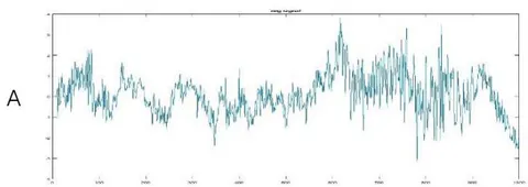
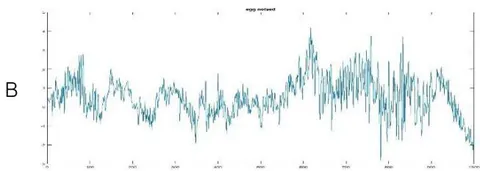
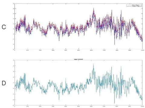
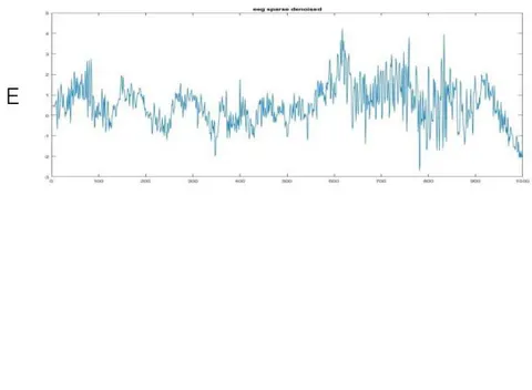
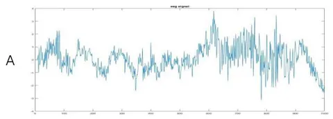
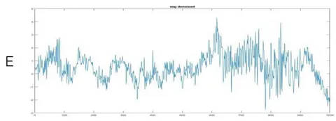
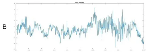
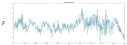
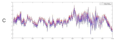
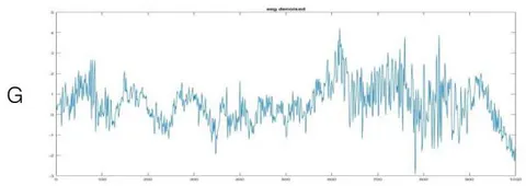
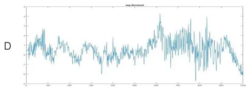
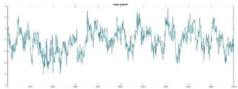
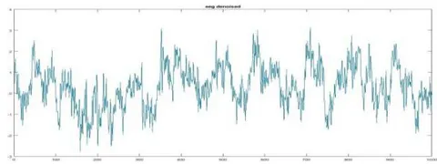
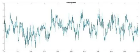
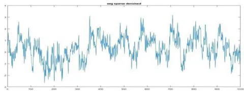
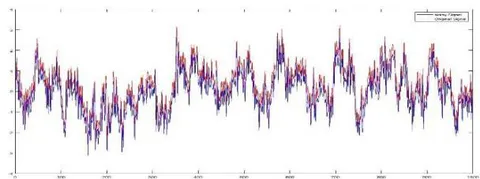
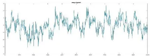
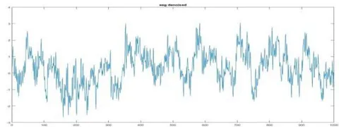
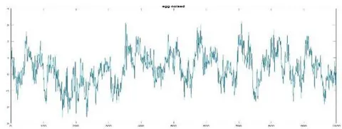
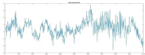
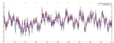
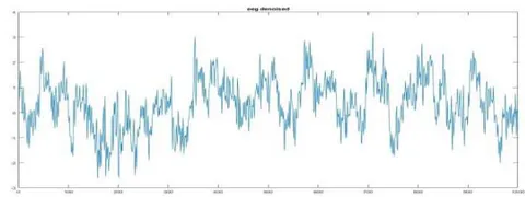
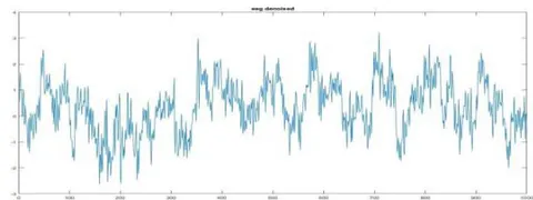
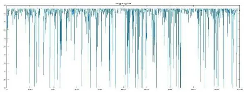
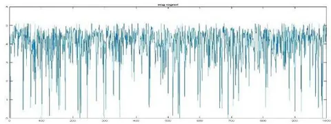
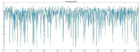
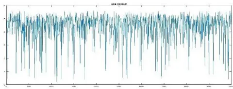
Electroencephalogram (EEG) [42], electrical action from the brain, one of the most vital signals from the human body, studying and improving this field of research is very important to physicians whose work is related to this branch of medicine, monitoring and observing changes in these signals help them to cover, predict, and cure brain diseases. In this example we applied the proposed mechanisms for denoising two different EEG signals, the results are shown in figure.1 for EEG signal 1, and figure.3 for EEG signal 2. The results for EEG signal 1 for the Gauss filter, Pow3 filter, Skew filter, and Tanh filter for EEG signal 1 are shown in figure.2, and in figure.4 for EEG signal 2, The performance is evaluated for all denoising algorithms using: Cross-Correlation (CC), the Mean Squared Error (MSE), Signal to Noise Ratio (SNR), Mean Absolute Error (MAE), and Peak Signal to Noise Ratio (PSNR), shown in table 1. The FWD and Sparse FWD have higher performance compared to other algorithms, while Sparse FWD is even better.

Dist.	Signal	(MSE)	(MAE)	(SNR)	(PSNR)	(CC)
Gauss	EEG1	0.1777	0.4141	7.5456	19.1214	0.9965
	EEG2	0.1769	0.4135	7.5440	16.2369	0.9966
Pow3	EEG1	0.1778	0.4140	7.5429	19.1187	0.9966
	EEG2	0.1758	0.4123	7.5695	16.2624	0.9968
Skew	EEG1	0.1753	0.4109	7.6033	19.1791	0.9962
	EEG2	0.1731	0.4066	7.6671	18.1044	0.9961
Tanh	EEG1	0.1757	0.4108	7.5946	19.1704	0.9963
	EEG2	0.1725	0.4072	7.5684	16.2613	0.9970
FWD	EEG1	0.1683	0.4017	7.7805	19.3563	0.9965
	EEG2	0.1695	0.4025	7.7631	19.1116	0.9968
Sparse FWD	EEG1	0.1673	0.3987	7.8071	19.3828	0.9967
	EEG2	0.1703	0.4050	7.7421	19.0906	0.9968

Example 2

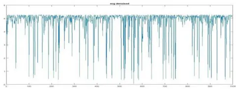
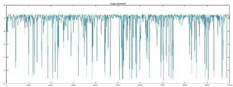
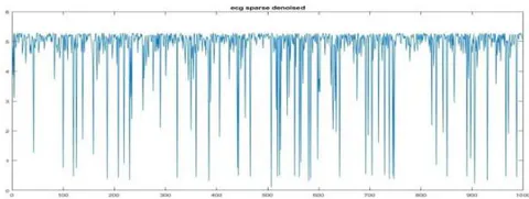
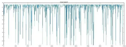
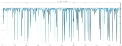
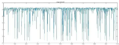
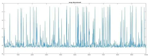
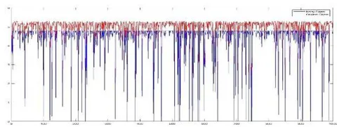
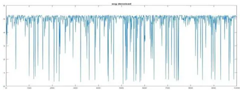
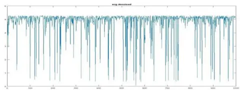
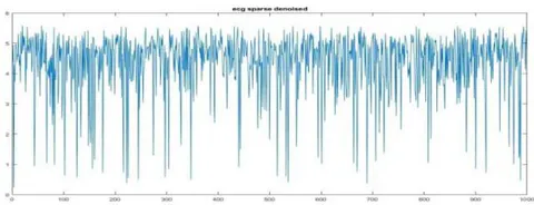
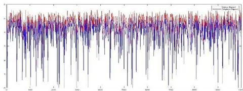
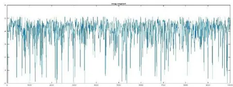
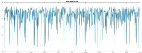
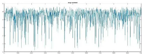
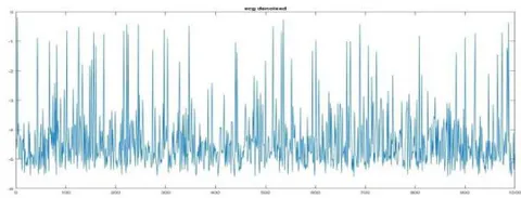
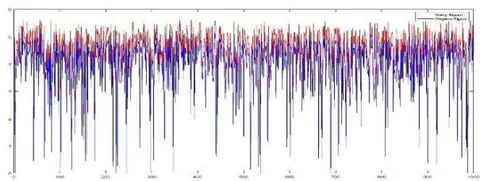
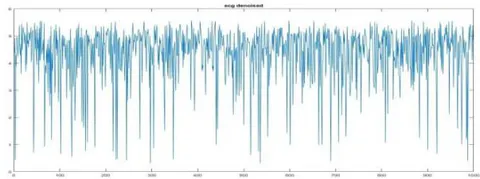
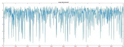
Electroencephalogram (ECG) [43], is an electrical activity from the heart that, like other types of biomedical signals, is frequently contaminated with various types of noise. In this example we used two mechanisms for denoising two different ECG signals, the FWD and the sparse FWD, the results are shown in figure.5 for ECG signal 1, and figure.7 for ECG signal 2,

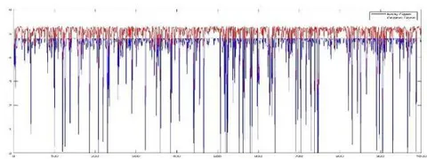
The results for ECG signal 1 for the Gauss filter, Pow3 filter, Skew filter, and Tanh filter for EEG signal 1 are shown in figure.6, and in figure.8 for EEG signal 2, Cross-Correlation (CC), Mean Squared Error (MSE), Signal to Noise Ratio (SNR), Mean Absolute Error

(MAE), and Peak Signal to Noise Ratio (PSNR) are used to evaluate the performance of all denoising algorithms, as shown in Table 2. When compared to other algorithms, FWD and Sparse FWD perform better, with Sparse FWD performing even better.

Dist.	Signal	(MSE)	(MAE)	(SNR)	(PSNR)	(CC)
Gauss	ECG1	0.1936	0.4326	20.1974	20.7429	0.9962
	ECG2	0.1745	0.4103	19.8627	21.7396	0.9965
Pow3	ECG1	0.1653	0.3976	20.8868	21.4323	0.9963
	ECG2	0.1668	0.3988	20.0631	21.9399	0.9961
Skew	ECG1	88.1655	9.1746	-6.3845	-5.8390	0.9969
	ECG2	74.1626	8.3769	-6.4173	-4.5405	0.9965
Tanh	ECG1	0.1707	0.4055	20.7445	21.2900	0.9965
	ECG2	0.1790	0.4163	19.7546	21.6315	0.9965
FWD	ECG1	0.1442	0.3712	21.4790	22.0245	0.9966
	ECG2	0.1424	0.3693	20.7510	22.6278	0.9967
Sparse FWD	ECG1	0.1468	0.3738	21.4014	21.9469	0.9971
	ECG2	0.1570	0.3873	20.3260	22.2029	0.9964

Example 3

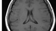
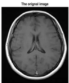
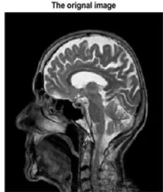
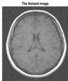
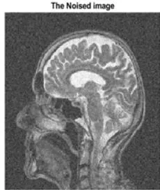
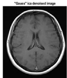
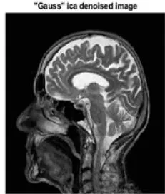
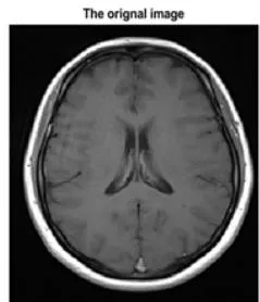
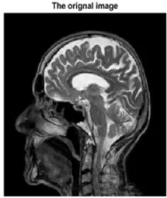
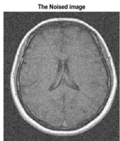
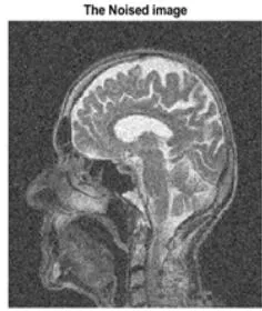
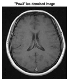
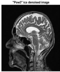
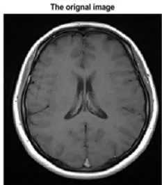
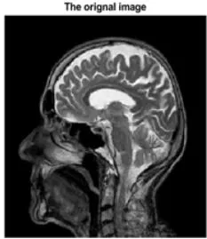
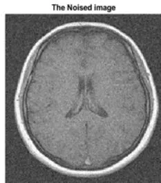
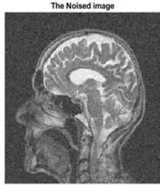
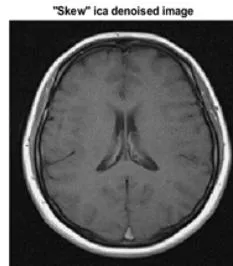
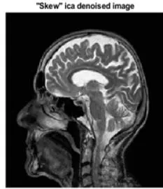
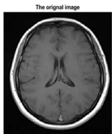
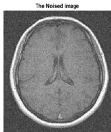
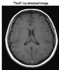
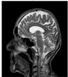
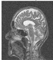
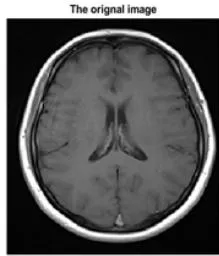
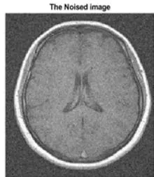
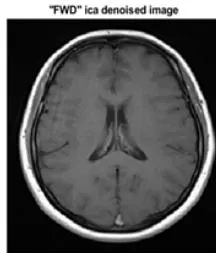
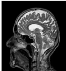
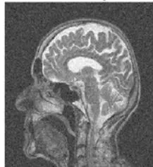
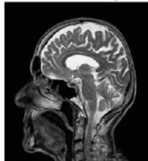
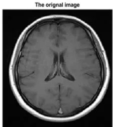
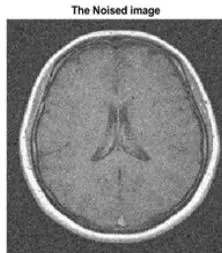
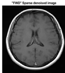
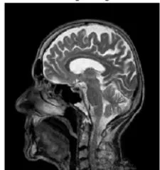
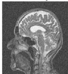
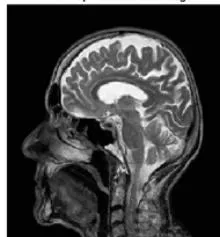
In this example, we show how our algorithm performed for both ICA and Sparse ICA techniques to denoise two medical images from [44]. Where Figures (9,10,11, and 12) show the original images, noised images, and denoised images after applying algorithms of Gauss, pow3, skew, and tanh. However, Figure 17 shows the denoising results for the FWD algorithm, and Figure 18 shows the denoising results for Sparse FWD; the results are illustrated in the Figures, and Table 3 shows the performance of these algorithms. FWD and Sparse FWD outperform other algorithms, with Sparse FWD outperforming them all.

Distribution/PSNR	First Image (Medical)			Second Image (Medical)			Elapsed time (in seconds)
	MSE	RMSE	PSNR	MSE	RMSE	PSNR
Gauss	0.0065	0.0079	85.0652	0.016	0.0128	80.9828	2.416944
Pow3	0.0083	0.0357	77.0871	0.091	0.0302	78.5261	4.316100
Skew	0.0072	0.0374	76.6692	0.051	0.0124	79.2583	2.340723
Tanh	0.0360	0.0188	82.6281	0.033	0.0180	83.0044	2.314567
FWD	0.0053	0.0073	90.8593	0.013	0.0117	86.7631	1.555153
Sparse FWD	0.0058	0.0076	90.4310	0.014	0.0122	86.3910	1.535551

A

D

B

E

C Fig. 3: FWD & Sparse FWD Filters (EEG signal 1): A original signal, B noised signal, C noised signal (original signal in blue and noise in red), D denoised signal (FWD), E denoised signal (Sparse FWD)

A

E

B

F

C

G

D Fig. 4: (EEG signal 2): A original signal, B noised signal, C noised signal (original signal in blue and noise in red), D denoised signal (Gauss filter), E denoised signal (Pow3 filter), F denoised signal (skew filter), G denoised signal (Tanh filter)

A

D

B

E

C Fig. 5: FWD & Sparse FWD Filters (ECG signal 1): A original signal, B noised signal, C noised signal (original signal in blue and noise in red), D denoised signal (FWD), E denoised signal (Sparse FWD)

A

E

B

F

C

G

D Fig. 6: (ECG signal 1): A original signal, B noised signal, C noised signal (original signal in blue and noise in red), D denoised signal (Gauss filter), E denoised signal (Pow3 filter), F denoised signal (skew filter), G denoised signal (Tanh filter)

A

D

B

E

C Fig. 7: FWD & Sparse FWD Filters (ECG signal 2): A original signal, B noised signal, C noised signal (original signal in blue and noise in red), D denoised signal (FWD), E denoised signal (Sparse FWD)

A

E

B

F

C

G

D Fig. 8: (ECG signal 1): A original signal, B noised signal, C noised signal (original signal in blue and noise in red), D denoised signal (Gauss filter), E denoised signal (Pow3 filter), F denoised signal (skew filter), G denoised signal (Tanh filter)

The original image

The Noised image

"Tanh"ica denoised image

The Noised image

"FWD" ica denoised image

The Noised image

"FWD" Sparse denoised image

VII. CONCLUSION

The fractional Weibull distribution and the sparse fractional Weibull distribution were used in this paper to introduce two mechanisms for medical signal denoising and blind source separation. In terms of denoising quality and computational cost, the mechanisms outperform existing solutions. We tested the mechanisms on two different types of biosignals (EEG signals and ECG signals) and two different types of medical images; the results were very good, and the mechanisms could be extended to work on other types of biosignals and medical images.

In future work, we aim to apply the algorithms to natural image denoising and mixed image separation.