## I. INTRODUCTION COVID-19 crises add up to several crises that have hit the globe. Counting the likes of World Warl and II and the great depression, the great recession, and Severe Acute Respiratory Syndrome Coronavirus 2 (SARS-CoV-2). The COVID-19 spread has travelled more than 150 countries and still spreading. By February 2021, globally, the pandemic had reached a case count of 113,467,303 people with a recorded death of 2,520,550 people (WHO, 2021). Governments all over the world have strived to contain the shocks. Countries across the globe adopted a series of containment measures to curb the spread of the novel coronavirus. Some of these strategies include the closure of borders and schools, restrictions on internal and international travel, washing hands with soap under running water with the aid of handwashing stations, use of hand sanitizer, social distancing, lockdown and the rest. These containment measures were to limit the spread of the virus but have unfortunately been attributed to the cause of shocks experienced by firms. Countries have succeeded through these containment measures to successfully rein the virus but unfortunately, the restrictions have hit firms' operations hard. In Africa, Agribusiness has been constrained in access to production inputs and a market for sales of products as a result of the restrictions imposed (Lakuma & Sunday, 2020). Markets were closed down, borders were closed, social distancing became a compulsory practice for everyone, and suspicion resulted in quarantines. Especially for small enterprises who could not innovate responsively to the shocks, they were either closed temporarily or recorded little sales, and hence large declines in business activities were more felt compared to the medium and large-scale enterprises (Lakuma & Sunday, 2020). The agricultural and manufacturing sectors have also suffered various levels of shocks. Business enterprises were encouraged to provide an enabling environment by the provision of handwashing centers and equipment, sanitizer, and lodging of employees within the premises of the business if they were to stay in business. The result of all these consequences have showcased in the massive unemployment rate across countries especially the fragile economies. If countries are to keep or increase the containment measures in a response to the risk pose by COVID 19, unemployment is will keep increasing denying a lot of households a livelihood. In the United State, unemployment shot up from $3.8\%$ to $13.5\%$ in May (Kochhar, 2020). The effect of the pandemic on Ghana is not far from the stories in other countries. This is because COVID-19 is a covariate risk and due to the lockdown of production and economic activities, countries do not benefit from cheaper oil and other commodities. The top ten most heat countries of COVID-19 include the United States of America, India, Brazil, Russia, Colombia, Peru, Spain, Mexico, Argentina, and South Africa. Below is the case count of COVID-19 worldwide by continent and country. By $28^{\text{th}}$ September, the world has reordered a total of thirty-three million cases with an average recovery of the rate of $74.5\%$ which varied across countries and continents from $0.3\%$ to $97.5\%$. Despite the fact that COVID-19 incidence is new, some newspapers and quite some articles like the work of Kahn et al. (2020) have given the subject area some discussions. Many corporate companies and national leadership of business interest have been interested in understanding sources of risk that could arise from this pandemic. Amidst the presence of COVID-19, the study seeks to forecast the volatility of the Ghana stock exchange composite index and examine the presence of asymmetry effect from the filtration of the bad news of fatal COVID-19 for the period October 2017 to February, 2021. This would serve as a yardstick to inform investors' decisions into the future with regards to the investment in the stock market in Ghana. As per the theories that underpin this study (i.e. efficient market theory and rational expectation intertemporal asset pricing theory), availability of market information is often in the prices of equities or stocks and as bad new filter the market, it is only rational to hold a less risky asset. The a priori anticipation of the study is that there will exist significantly high volatility and that asymmetric effect will be negative and significant (Kahn et al., 2020). This study will help to firms, investors, and policymakers to know the extent to how risky Ghana stock exchange composite index is and how the index will be shortly. Policymakers and regulators need to know the forecast of the future trend of the stock market to formulate polices based on that empirical findings. ## II. LITERATURE REVIEW The pandemic is reported to have a severe impact on economies all over the world. The pandemicis said to contract the global economy by $3\%$ which is worse than the previously experienced global crises (World Economic Outlook, 2020). The world came to know of the deadly COVID- 19 when the Wuhan Municipal Health Committee officially announced to the World Health Organisation that a "new pneumonia-like disease of unknown cause" detected in Wuhan, the capital city of Hubei province of China. Governments across the globe had to implement a wide range of policies aimed at protecting workers and supporting businesses to survive the shocks of the pandemic. Containment and economic recovery policies have been in the minds the central government and local governments at the provincial and municipal levels. These policies and long-ranging on tax policies, employment policies, financial policies, health policies, and international trade policies. In the United State of America, monetary and macro-financial policies touched on lowering the federal fund rate by 150bp in March to 0-0.25bp. the cost of discount window lending was reduced and the existing cost of swapping lines with major central banks was also reduced. There was an extension of the maturity of FX operations with a broadened US dollar swap lines to more centralbanks. In Ghana, the containment measures adopted by the government include banding of all kinds of social gathering exceeding 25 people for four weeks; closure of all universities and schools until further notice; closure of borders to travelers; and mandatory 14 - day self-quarantine for any Ghanaian who has been to a country with at least 200 confirmed cases of COVID-19. In the fiscal fonts, as the government intends to commit an amount of GHS 11.2 billion to face COVID-19 and its related social and economic hardships dubbed Coronavirus Alleviation Programme, large government spending has been cut on all economic classifications of government budgeted annual expenditures such as goods and services, transfers, and capital investments. The Coronavirus Alleviation Programme is intended to be used to support industries in the pharmaceutical sector supplying COVID-19 drugs, and equipment, support SMEs, build or upgrade 100 district and regional hospitals and address the availability of test kits, pharmaceuticals, equipment, and bed capacity. To finance pressing needs that COVID 19 has created, the government intends to borrow GH¢ 10 billion from the Bank of Ghana has drawn an amount of US$ 218 million from the stabilization fund. In the monitory and macro-financial sector, the policy rate was cut by 150 basis points to $14.5\%$. as part of efforts in mitigating the effect of the pandemic, the Monetary Policy Committee of Ghana lowered the primary reserve requirement and capital conservation buffer from $10\%$ to $8\%$ and $3\%$ to $1.5\%$ respectively. The cost of mobile payment was also lowered and was accordingly complied by both Banking and Non-Banking financial institutions. There were unfortunately no polices on the exchange rate and balance of payment level. In line with the focus of this study, Kahn et al., (2020) examined the impact of the COVID-19 pandemic on stock markets sixteen countries and found that investors in these countries react to the bad news of the pandemic at the early stage. GPD is claimed to be significantly impacted due to a decline in production among firms (Wren-Lewis, 2020). If the pandemic persists with its magnitude and fatality, Banks will soon fail to meet the financial requirement of firms which will cause the breakdown of the stock markets. The overall downturn in global production as a result of the lockdown of firms and industries risk increasing prices of essential commodities shortly. ## III. STUDY METHODOLOGY The study employed the Autoregressive Integrated Moving Average (ARIMA) model to forecast the Ghana Stock exchange composite index after a period of the 8-months of shock of COVID-19 to Ghana and the world at large. The ARIMA model is also sometimes called the Box Jenkins (2019) methodology. The model uses information derived from its past behaviors to forecast its trend. It is a univariate model and where the variable itself is regressed on its pass value. It uses the philosophy of "let variable speak for itself". There are two underlying assumptions of ARIMA modeling. The first assumption is a concern with the stationarity of the time series in question. The series must exhibit mean reversions, has infinite, and time-invariant variance and must also have a theoretical correlogram that diminishes as the lag length increases. The second is the invertibility assumption which requires that the series should be able to be represented by a finite order MA or convergent autoregressive process. It is also the ACF and PACF for identification. It also implicitly assumes that the series can be approximated by the AR model. ### a) Specification of the ARIMA Model ARIMA model allows a series say $Y_{t}$ to be regressed by lagged values of the same series and error term. As a result, it is often called atheoretic model since it is not obtained from any economic theory. RIMA is composed of an AR model and a MA model. Consider the equation below. $$ Y _ {t} = a + b Y _ {t - 1} + u _ {t} \tag {1} $$ $$ Y_{t} = a + b(LY) + u_{t} \mathrm{or} (1 - bL) = a + u_{t} $$ where $a$ and $u_{t}$ denote constant and stochastic white noise respectively. $Y_{t}$ is the Ghana stock exchange composite index. A key assumption of ARIMA modeling is stationarity and so it is assumed that $|b| > 1$, the composite index will tend to be bigger and bigger at each period time and the composite index will become explosive. More lags can be included as a generalization of the AR model. For instance, an AR (2), AR (3), and AR(p) is given as; $$ \mathrm {A R} (2) \colon Y _ {t} = a + b _ {1} Y _ {t - 1} + b _ {2} Y _ {t - 2} + u _ {t} $$ $$ \operatorname{AR}(3): Y_{t} = a + b_{1}Y_{t-1} + b_{2}Y_{t-2} + b_{3}Y_{t-3} + u_{t} \tag{2} $$ $$ \operatorname{AR}(p): Y_{t} = a + \sum_{q}^{p} b_{i} Y_{t-i} + u_{t} $$ For a moving average model, the composite index is explained by the value of the error term and the immediate past error term. An MA(1), MA(2) and MA(p) can be specified as; $$ \mathrm {M A} (1) \colon Y _ {t} = \gamma + d _ {0} u _ {t} + d _ {1} u _ {t - 1} $$ $$ \mathrm{MA}(2)\colon Y_{t} = \gamma + d_{0}u_{t} + d_{1}u_{t-1} + d_{1}u_{t-2} \qquad (3) $$ $$ \mathrm{MA}(p)\colon Y_{t} = \gamma + d_{0}u_{t} + \sum_{j}^{q} d_{j}u_{t-j} $$ Combining the AR(q) and AR(q) we obtain Autoregressive Moving Average (ARMA) specified in equation (4). $$ \operatorname{ARMA} (p, q): Y _ {t} = a + \sum_ {i} ^ {p} b _ {i} Y _ {t - i} + d _ {0} u _ {t} + \sum_ {j} ^ {q} d _ {j} u _ {t - j} \tag{4} $$ where $p$ lags of the dependent variable and $q$ lags of the error term. Most economic variables are non-stationary and so ARIMA brings in the case of integration of the variable which is not stationary. The difference between ARMA and ARIMA and the integration of the dependent variable. In real-life situations, most time series variables are not stationary and therefore will need to be transformed to be stationary. The ARIMA model can be specified in different ways depending on the lag(s) of the AR and MA. ARIMA $(p, d, q)$ implies there are $p$ number of lags of the dependent variable, the variable has been differenced $d$ times to become stationary and there are $q$ lags of the error term. Parsimoniousmodels give a better forecast than over parameterized model. Therefore, it is important to pick themodels with the smallest number of parameters to be estimated. ### b) Identification of the ARIMA model The identification involves the selection of the ideal lags for the AR and MA process. It is usually done using the correlogram. The correlogram is simply the plots of the ACFs and PACFs against the lad length. PACF measures the correlation between observations that are $k$ time period apart after controlling for correlations at immediate lags. It is important to know the pattern of ACF and PACF before one can decide whether the series is going to follow an AR process, MA process, or a combination of an AR and MA. To know whether it is going to be an ARIMA, Table 2 presents provides a guide to aid one in choosing an appropriate ARIMA model. Table 2: Guide for Identification <table><tr><td>Model</td><td>ACF Pattern</td><td>PACF Pattern</td></tr><tr><td>AR(p)</td><td>Exponential decay or damped sine wave pattern or both</td><td>Significant spikes through first lag</td></tr><tr><td>MA(q)</td><td>Significant spikes through first lag</td><td>Exponential decays</td></tr><tr><td>ARMA (1,1)</td><td>Exponential decays from lag 1</td><td>Exponential decays from lag 1</td></tr><tr><td>ARMA(p,q)</td><td>Exponential decays</td><td>Exponential decays</td></tr></table> ### c) Exponential GARCH Model Exponential GARCH also found out whether the bad news COVID-19 which filtered every part of the world and for that matter Ghana had a significant shock on the volatility of the Ghana stockexchange composite index. The GARCH model was introduced by Tim Bollerslev in 1986 and has been employed by many economists and financial analysts. Following Sunarya (2019), we specify GARCH(1,1) in equation (5) as; $$ h_{t} = \varphi + \theta_{1} h_{t-1} + b_{1} u_{t-1}^{2} \qquad (5) $$ where $h_t$ is the conditional variance, $t$ denotes time, and $u_{t-1}^2$ is the lagged squared error term. The model spelifes that the conditional variance at time $t$ depends on both the past values of the shocks captured by lagged squared error terms and past figures of itself. The GARCH $(p,q)$: $h_t$ model whengeneralized becomes; $$ \mathrm{GARCH}(p,q)\colon h_{t} = \varphi + \sum_{k}^{p} \theta_{k} h_{t-k} + \sum_{i}^{q} b_{i} u_{t-i}^{2} (6) $$ where $P = 0$, equation (6) reduces to $\operatorname{ARCH}(q)$. Drawing insights from GARCH and threshold GARCH, Nelson (1995) introduced exponential GARCH to capture the test for asymmetries. When bad news filter into the market, assets tend to enter into a state of turbulence and volatility increases. Unlike the case of the TGARCH, the EGARCH uses the log of the series as the dependent variable and not the levels. The conditional variance for the EGARCH $(p,q)$ model is given as; $$ \log (h _ {t}) = \varphi + \sum_ {i = 1} ^ {q} \eta_ {i} \left| \frac{u _ {t - i}}{\sqrt{h _ {t - i}}} \right| + \sum_ {i = 1} ^ {q} \lambda_ {i} \left| \frac{u _ {t - i}}{\sqrt{h _ {t - i}}} \right| + \sum_ {k = 1} ^ {p} \theta_ {k} \log (h _ {t - k}) \tag{7} $$ Where $\log (h_t)$ denotes the log of the variance series, which makes the leverage effect exponential instead of quadratic. The implication is that the estimates are non-negative. $\mathsf{V}$ denotes the constant, $\eta$ represents the ARCH effects, $\lambda$ denotes the asymmetric effect, and $\theta$ represents the GARCH effect. The condition is that if $\lambda_1 = \lambda_2 = \dots = 0$, the model is symmetric. However, where $\lambda_i < 0$, it implies that negative shocks generate larger volatility than good news. ### d) Diagnostics test for the EGARCH The preferred model must have the following features; the model must be parsimonious; the ARCH and GARCH coefficients must be statistically significant; the adjusted R-square and the log-likelihood ratio must be high; the SIC information criterion which gives the heaviest penalties for loss of degrees of freedom must be low; and must pass both heteroscedasticity and autocorrelation test. Every model may not pass all these specifications but there could be a reasonable tradeoff. In GARCH diagnostics, a normality test is not necessary because, by nature, the GARCH model have fat tails and are either skewed to the left or right. ## IV. 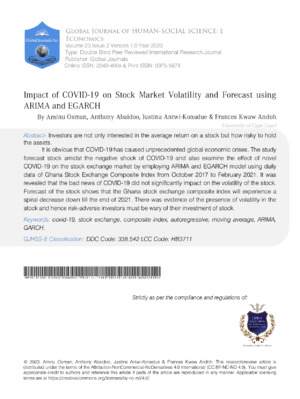RESULTS AND DISCUSSIONS The plot of the GSECI for the period under study is shown in figure 1. The series is observed to be declining sharply from the last quarter of 2018 and continues to depict a slow downward trend till quarter four of 2019 where it gained some momentum increased slightly. At the beginning of 2020, the GSECI showed a downward trend from quarter one to quarter three.   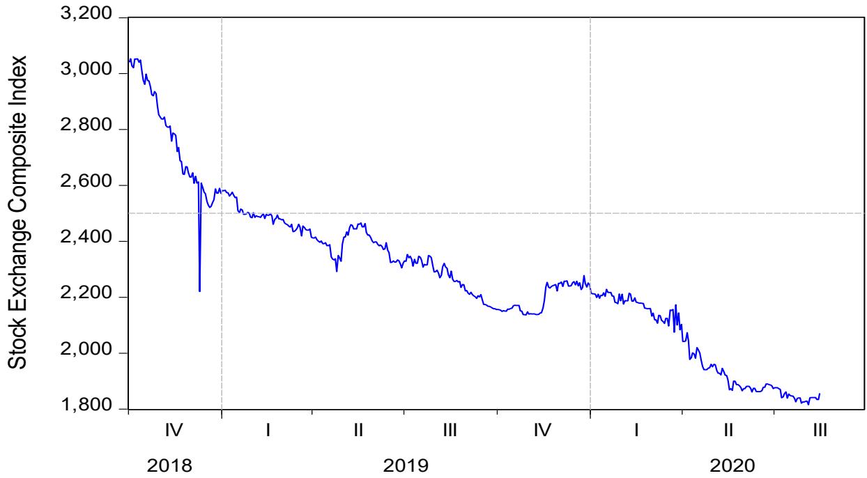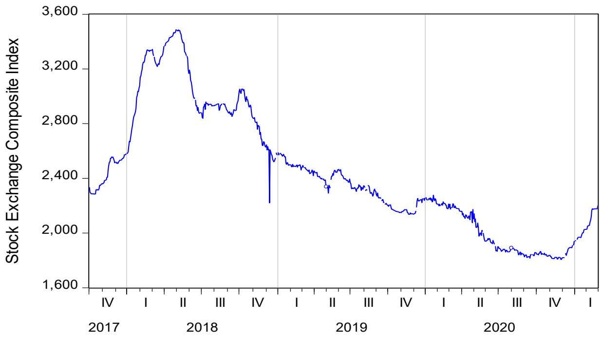Figure 1: Historical Plots of GSECI The plot of the historical daily GSECI shows that the series is trending downwards and not reverting to its mean. By visualizing it, we say the series is nonstationary. fluctuates around some common mean and ### a) Unit Root Test for Stationarity therefore it is non-stationary. This is confirmed with the use of the Dickey-Fuller test for unit root presented in Table 1. Table 1: ADF test statistics <table><tr><td rowspan="2">IGSECI</td><td colspan="2">I (0)</td><td colspan="2">I (1)</td></tr><tr><td>t-Statistic</td><td>P-value</td><td>t-Statistic</td><td>P-value</td></tr><tr><td>AIC</td><td>-3.366978</td><td>0.0566</td><td>-5.599723</td><td>0.0000</td></tr><tr><td>SIC</td><td>-3.242959</td><td>0.0769</td><td>-6.149055</td><td>0.0000</td></tr><tr><td>HQC</td><td>-3.366978</td><td>0.0566</td><td>-5.599723</td><td>0.0000</td></tr></table> Table 1 presents the test for unit roots of the series using all the criteria (i.e. Akaike Information Criterion, Schwarz Info Criterion, and Hanna-Quin Criteria). For all the criterion at the intercept and trend, it is found that the daily series of Ghana Stock exchange composite index for the period under study is not stationary at $5\%$ level and therefore the series must be transformed. It is confirmed by using a correlogram. With the aid of a correlogram, we check for stationarity. In Appendix 1, it is found that the series is not stationary at level since the ACF declines very slowly up to about 36 lags. It showed a significant autocorrelation that is outside the error bounds and decays slowly. It is indicative that the series is nonstationary since they are outside the standard error bounds or confident interval at $95\%$. The PACF also drops immediately after the first and second lag continuously. The series is therefore not stationary.   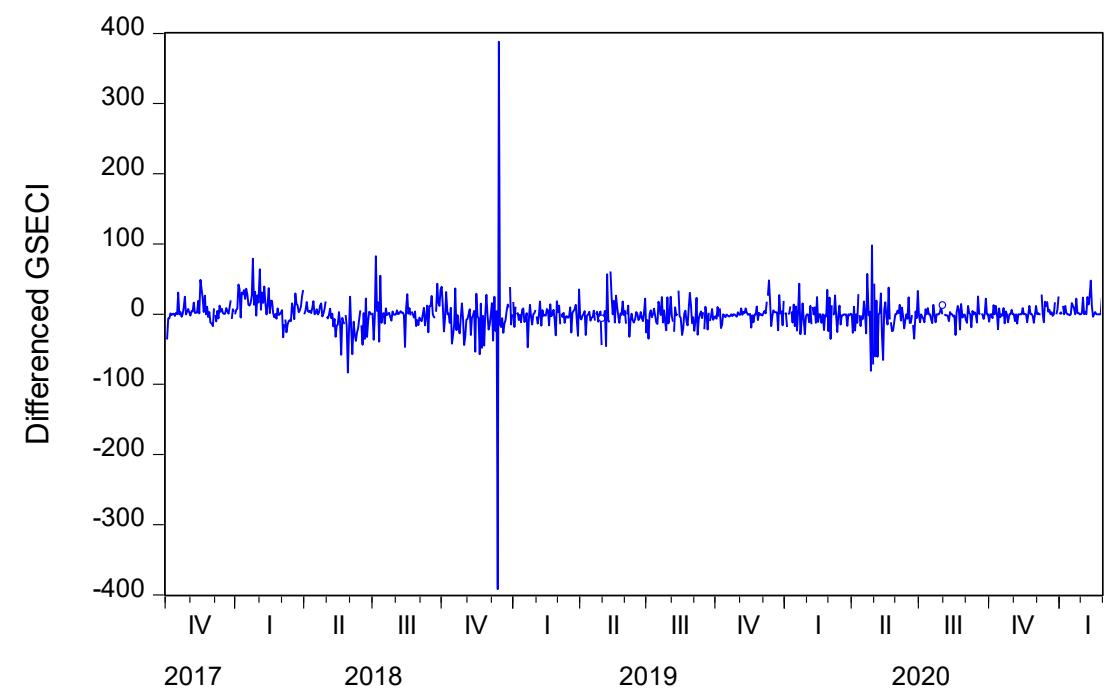Figure 2: Plot of transformed GSECI After first differencing, the series shown in Figure 2, is now mean-reverting. That is, the GSECI is now integrated of order one, I (1). ### b) Estimatesof ARIMA Model ARIMA informs that the series in question has gone through an integration process before being used for any analysis. Before deciding on the appropriate ARIMA model to be used for the data sequence, Figure 1 presents the correlogram plots of the differenced GSECI which indicates the level of significance of the Q-statistics of a specific set of lags from one to inform our decision on the ideal ARIMA model. The decision on the appropriate lags for the ARIMA model is to arrive using the Autocorrelation Function (ACF) and the Partial Autocorrelation Function (PACF). The autocorrelation of the first difference of the Ghana stock exchange composite index shows that at the lag one, the ACF is significant and shows an exponential decay till lag 4 where the ACF extends beyond the confidence interval bounds and continue decaying exponentially. There exists a slight similarity between the ACF and the PACF (see Appendix 2 for the correlogram). Since the pattern of the ACF and PACF looks the same, we can conclude having a set of tentative ARIMA models (1,1,1), ARIMA (1,1,4), ARIMA (4,1,1) and ARIMA (4,1,4). It is advised to choose a model that is parsimonious as it gives a better forecast than an overidentified model. Models with the smallest number of parameters to be estimated are usually parsimonious. From Table 2, between the contest ARIMA (1,1,1) and ARIMA (4,1,1) which all have 2 significant coefficients, ARIMA (4,1,1) is ideal for the study since it has the lowest volatility, highest adjusted R-square, and lowest AIC and SBIC. Table 2: Determination of Appropriate ARIMA Model <table><tr><td>Differenced GSECI</td><td>ARIMA (1,1,1)</td><td>ARIMA (4,1,1)</td><td>ARIMA (1,1,4)</td><td>ARIMA (4,1,4)</td></tr><tr><td>Significant coefficient</td><td>2</td><td>3</td><td>3</td><td>3</td></tr><tr><td>Sigma2(volatility)</td><td>619.0792</td><td>599.9418</td><td>599.9776</td><td>651.5751</td></tr><tr><td>Adj R2</td><td>0.080375</td><td>0.108803</td><td>0.108750</td><td>0.032103</td></tr><tr><td>AIC</td><td>9.275762</td><td>9.244577</td><td>9.244561</td><td>9.327075</td></tr><tr><td>SBIC</td><td>9.298344</td><td>9.267160</td><td>9.267144</td><td>9.349658</td></tr></table> ### c) ARIMA Model Estimate The final model has been determined as ARIMA (4,1,1) and it is presented in Table 3. Table 3: ARIMA (4,1,1) estimates of the Ghana Stock Exchange Composite Index. <table><tr><td>Variable</td><td>Coefficient</td><td>Std. Error</td><td>t-Statistic</td></tr><tr><td>Constant</td><td>-0.161561</td><td>0.976326</td><td>-0.165478</td></tr><tr><td>AR (4)</td><td>0.212911***</td><td>0.014475</td><td>14.70849</td></tr><tr><td>MA (1)</td><td>-0.287736***</td><td>0.007387</td><td>-38.94937</td></tr><tr><td>SIGMASQ</td><td>599.9418***</td><td>5.705647</td><td>105.1488</td></tr></table> ### d) Forecast analysis of GSE-Cl The ARIMA (4,1,1) model is used to forecast the closing price of the Ghana stock exchange composite index from $1^{\text{st}}$ March, 2021 to $26^{\text{th}}$ February, 2022. The forecast of the outer year from March 2021 to February 2022 shows a upwards trend of the GSECI.  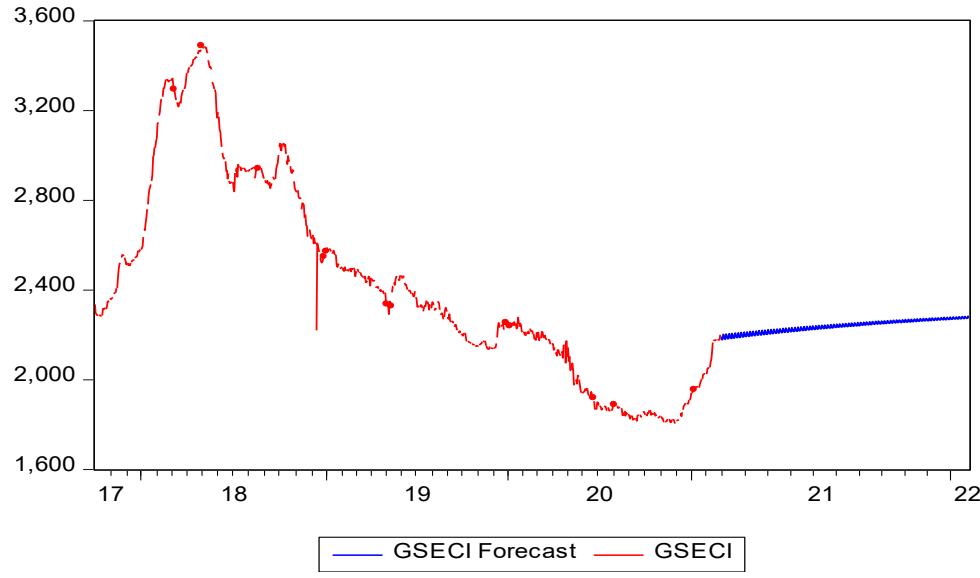Figure 3: Forecast of GSECI showing Actual and Forecast The correlogram after estimation of the ARIMA (4,1,1) model indicates there is no information uncaptured since all the residuals are barely flat and do not lie above the standard error bound. Thus, all the lag structures should lie within the $95\%$ confidence intervals or the standard error bounds. Since all the residuals lie within the standard error bounds, we can conclude that ARIMA $(4,1,1)$ is appropriate. Figure 3 presents the Ljung-Box test for squared residuals; no lag is found to be significant in the correlogram of the residual and hence there is no information leftuncaptured. Figure 4: Correlogram after estimation of ARIMA (4,1,1)Exponential GARCH (1,1) <table><tr><td>Autocorrelation</td><td>Partial Correlation</td><td>AC</td><td>PAC</td><td>Q-Stat</td><td>Prob</td></tr><tr><td>□</td><td>□</td><td>1</td><td>-0.288</td><td>-0.288</td><td>69.788</td></tr><tr><td>□</td><td>□</td><td>2</td><td>0.104</td><td>0.023</td><td>78.953</td></tr><tr><td>□</td><td>□</td><td>3</td><td>-0.005</td><td>0.034</td><td>78.973</td></tr><tr><td>□</td><td>□</td><td>4</td><td>0.165</td><td>0.185</td><td>101.88</td></tr><tr><td>□</td><td>□</td><td>5</td><td>-0.003</td><td>0.101</td><td>101.89</td></tr><tr><td>□</td><td>□</td><td>6</td><td>0.110</td><td>0.129</td><td>112.04</td></tr><tr><td>□</td><td>□</td><td>7</td><td>0.065</td><td>0.130</td><td>115.65</td></tr><tr><td>□</td><td>□</td><td>8</td><td>0.080</td><td>0.109</td><td>121.05</td></tr><tr><td>□</td><td>□</td><td>9</td><td>0.037</td><td>0.069</td><td>122.20</td></tr><tr><td>□</td><td>□</td><td>10</td><td>0.042</td><td>0.022</td><td>123.70</td></tr><tr><td>□</td><td>□</td><td>11</td><td>0.013</td><td>-0.028</td><td>123.84</td></tr><tr><td>□</td><td>□</td><td>12</td><td>0.086</td><td>0.026</td><td>130.16</td></tr><tr><td>□</td><td>□</td><td>13</td><td>0.016</td><td>-0.001</td><td>130.37</td></tr><tr><td>□</td><td>□</td><td>14</td><td>0.034</td><td>-0.013</td><td>131.38</td></tr><tr><td>□</td><td>□</td><td>15</td><td>0.027</td><td>-0.006</td><td>132.02</td></tr><tr><td>□</td><td>□</td><td>16</td><td>0.077</td><td>0.045</td><td>137.07</td></tr><tr><td>□</td><td>□</td><td>17</td><td>-0.032</td><td>-0.026</td><td>137.94</td></tr><tr><td>□</td><td>□</td><td>18</td><td>0.020</td><td>-0.037</td><td>138.30</td></tr><tr><td>□</td><td>□</td><td>19</td><td>0.006</td><td>-0.036</td><td>138.33</td></tr><tr><td>□</td><td>□</td><td>20</td><td>0.060</td><td>0.015</td><td>141.39</td></tr><tr><td>□</td><td>□</td><td>21</td><td>-0.011</td><td>-0.002</td><td>141.50</td></tr><tr><td>□</td><td>□</td><td>22</td><td>0.000</td><td>-0.030</td><td>141.50</td></tr><tr><td>□</td><td>□</td><td>23</td><td>0.012</td><td>-0.012</td><td>141.61</td></tr><tr><td>□</td><td>□</td><td>24</td><td>0.019</td><td>0.000</td><td>141.92</td></tr><tr><td>□</td><td>□</td><td>25</td><td>-0.021</td><td>-0.020</td><td>142.29</td></tr><tr><td>□</td><td>□</td><td>26</td><td>-0.029</td><td>-0.054</td><td>142.99</td></tr><tr><td>□</td><td>□</td><td>27</td><td>0.047</td><td>0.016</td><td>144.88</td></tr><tr><td>□</td><td>□</td><td>28</td><td>0.035</td><td>0.058</td><td>145.97</td></tr><tr><td>□</td><td>□</td><td>29</td><td>0.005</td><td>0.054</td><td>145.99</td></tr><tr><td>□</td><td>□</td><td>30</td><td>-0.012</td><td>0.022</td><td>146.11</td></tr><tr><td>□</td><td>□</td><td>31</td><td>-0.020</td><td>-0.027</td><td>146.45</td></tr><tr><td>□</td><td>□</td><td>32</td><td>-0.021</td><td>-0.057</td><td>146.83</td></tr><tr><td>□</td><td>□</td><td>33</td><td>0.040</td><td>0.015</td><td>148.24</td></tr><tr><td>□</td><td>□</td><td>34</td><td>-0.003</td><td>0.012</td><td>148.25</td></tr><tr><td>□</td><td>□</td><td>35</td><td>-0.007</td><td>-0.013</td><td>148.30</td></tr><tr><td>□</td><td>□</td><td>36</td><td>-0.001</td><td>-0.015</td><td>148.30</td></tr></table> ### e) Exponential GARCH (1,1) The coefficient of interest is the asymmetric term. The term is positive (0.2983) and significant at $1\%$ level. This means that at the time of computation of the results, bad news from COVID-19 has failed to significantly aggravate the behavior of the stock exchange composite index. The outbreak and the bad news of COVID-19 pandemic does not significantly determine the volatility of the Ghana Stock Exchange Composite Index. Table 4: Estimate of EGARCH (1,1) of GSECI <table><tr><td>Variable</td><td>Coefficient</td><td>Std. Error</td><td>t-Statistic</td></tr><tr><td>Constant</td><td>-1.203569**</td><td>0.503448</td><td>-2.390653</td></tr><tr><td>ARCH</td><td>0.505702***</td><td>0.150296</td><td>3.364698</td></tr><tr><td>Asymmetric</td><td>-0.03326</td><td>0.089315</td><td>-0.372384</td></tr><tr><td>GARCH</td><td>0.894308***</td><td>0.050997</td><td>17.53663</td></tr><tr><td>R-squared</td><td>0.996476</td><td>Mean dependent var</td><td>7.779222</td></tr><tr><td>Adjusted R-squared</td><td>0.996472</td><td>S.D. dependent var</td><td>0.180569</td></tr><tr><td>Log likelihood</td><td>3162.471</td><td>Akaike info criterion</td><td>-7.530956</td></tr></table> The exponential terms $(\exp^{0.03326} = 1.2156646)$ indicate that for the Ghana Stock exchange composite index, the bad news of COVID-19 has a rather large symmetric effect on the volatility of the stock. The exponential term was however not significant even at 10% level. But for the insignificance of the asymmetric term, negative shocks invoke greater volatility than a positive shock. The bad news of the COVID-19 did not influence the volatility of the stock exchange. ### f) EGARCH Diagnostics Table 5: Diagnostic test of Appropriateness <table><tr><td>Logged GSECI</td><td>Normal Gaussian</td><td>Student t&#x27;s</td><td>GED</td><td>Student&#x27;s twith fixed df</td></tr><tr><td>Significant Coefficient s</td><td>All*</td><td>2</td><td>2</td><td>3</td></tr><tr><td>ARCH Significance</td><td>Yes</td><td>Yes</td><td>Yes</td><td>Yes</td></tr><tr><td>GARCH Significance</td><td>Yes</td><td>Yes</td><td>Yes</td><td>Yes</td></tr><tr><td>Log-likelihood</td><td>2758.957</td><td>3074.970</td><td>3162.471*</td><td>3020.470</td></tr><tr><td>Adj R²</td><td>0.996443</td><td>0.996469</td><td>0.996472*</td><td>0.996472</td></tr><tr><td>Schwarz IC</td><td>-6.536429</td><td>-7.282604</td><td>-7.491437*</td><td>-7.160566</td></tr><tr><td>Heteroscedasticity</td><td>No</td><td>No</td><td>No</td><td>No</td></tr><tr><td>Autocorrelation</td><td>Yes</td><td>Yes</td><td>Yes</td><td>Yes</td></tr></table> In choosing the preferred model, we depend on the four different error constructs in Table 5 above. The model must be parsimonious. Thus, the ARCH and GARCH coefficients must be statistically significant. The generalized error model has the highest adjusted R-square and the log-likelihood ratio. The Generalized Error Distribution (GED) model also the lowest SIC information criterion which gives the heaviest penalties for loss of degrees of freedom. All the models have the same results for test of heteroscedasticity and serial correlation. The reasonable tradeoff is to choose the generalized error distribution model. From the GARCH (1,1) model in Table 4, both the GARCH and ARCH models are positive and significant at one $1\%$ level. The residual test reveals that the model passes the residual test since the F-statistic is not significant at $1\%$ level. From Table 5, there is no evidence of heteroscedasticity in the residuals. Using the correlogram Q-statistics, there existed no serial correlation in the residuals. The ACF and the PACF lie within the confidence intervals as shown in Figure 2. There exist no probability values of the Q-statistics below the alpha level of $1\%$ indicating that there is no serial correlation. Evidence of serial correlation here is when the p-values of the Q-statistics are statistically significant.   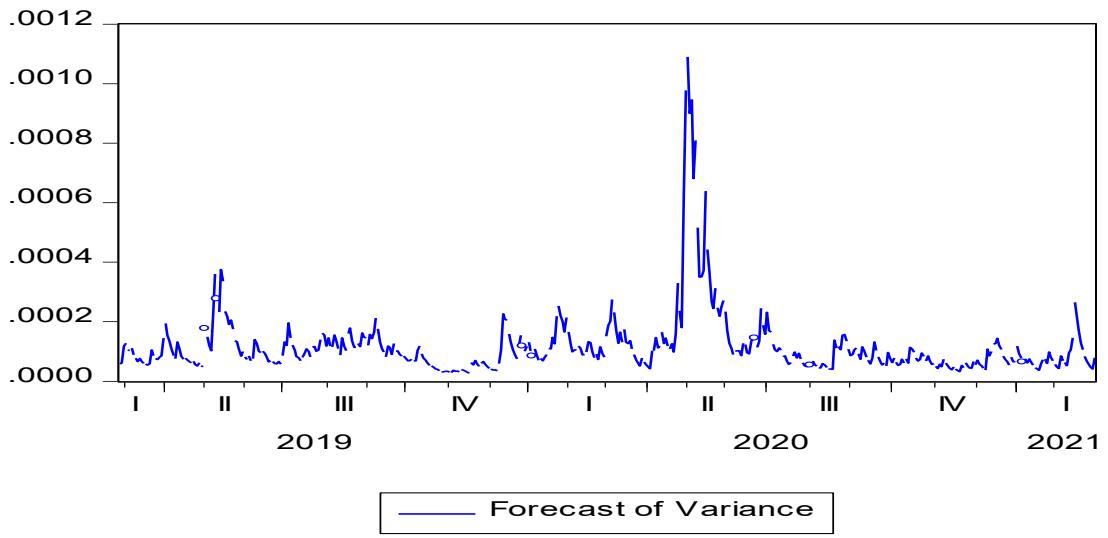Figure 6: Static Plot of Forecast ### g) EGARCH Forecast of GSECI Not much information was obtained from the dynamic forecast of using the EGARCH model. As a result, a static forecast was used and the results are shown in Figure 5. We can conclude from the plot that the return of GSECI is stable but shows intense volatility. Thought it is sown that return on the composite index will be stable over time, there is exist turbulence throughout the period and we can predict that volatility may occur for the outer days, months, and years. Volatility towards the end of the years still shows high volatility. Volatility during the period of COVID-19 was intense in the second quarter of 2020. Volatility was very severe from May to June but slowed in July and become extremely high and slowed towards the end of August 2020. The volatility measures the risky involve when an investor holds an asset in such a stock exchange market. ## V. CONCLUSION The study found that the GSECI data is nonstationary for the period October, 2018 to February 2021. It becomes stationary after first differencing of the original GSECI data. After the comparison made with several tentative models, ARIMA (4,1,1) is found to be ideal for the study. The period of bad news of the COVID-19 adds to the declining trend of the composite index whose volatility begun to subsides towards the end of August, 2020 with some slight turbulence in the first two months of 2021. This might be due to the rising in the COVID-19 case count which hit Ghana after the 2020 General Election on $7^{\text{th}}$ December. The high volatility of the composite index in the EGARCH shows that investors should be careful of the risky nature of the assets since it is very irrational to invest in assets that will not provide a sure profit. However, since the volatility is beginning to slow in the early 2021, investors can be ready to make informed decisions on the index. <table><tr><td>Date</td><td>Forecast Value</td><td>Date</td><td>Forecast Value</td><td>Date</td><td>Forecast Value</td></tr><tr><td>4/10/2020</td><td>2000.80</td><td>10/9/2020</td><td>1733.08</td><td>4/9/2021</td><td>1414.09</td></tr><tr><td>4/13/2020</td><td>1996.79</td><td>10/12/2020</td><td>1730.63</td><td>4/12/2021</td><td>1411.64</td></tr><tr><td>4/14/2020</td><td>1981.93</td><td>10/13/2020</td><td>1728.17</td><td>4/13/2021</td><td>1409.19</td></tr><tr><td>4/15/2020</td><td>2019.68</td><td>10/14/2020</td><td>1725.72</td><td>4/14/2021</td><td>1406.73</td></tr><tr><td>4/16/2020</td><td>2011.97</td><td>10/15/2020</td><td>1723.27</td><td>4/15/2021</td><td>1404.28</td></tr><tr><td>4/17/2020</td><td>2000.12</td><td>10/16/2020</td><td>1720.81</td><td>4/16/2021</td><td>1401.83</td></tr><tr><td>4/20/2020</td><td>1975.81</td><td>10/19/2020</td><td>1718.36</td><td>4/19/2021</td><td>1399.37</td></tr><tr><td>4/21/2020</td><td>1952.12</td><td>10/20/2020</td><td>1715.90</td><td>4/20/2021</td><td>1396.92</td></tr><tr><td>4/22/2020</td><td>1941.03</td><td>10/21/2020</td><td>1713.45</td><td>4/21/2021</td><td>1394.47</td></tr><tr><td>4/23/2020</td><td>1941.03</td><td>10/22/2020</td><td>1711.00</td><td>4/22/2021</td><td>1392.01</td></tr><tr><td>4/24/2020</td><td>1941.03</td><td>10/23/2020</td><td>1708.54</td><td>4/23/2021</td><td>1389.56</td></tr><tr><td>4/27/2020</td><td>1946.14</td><td>10/26/2020</td><td>1706.09</td><td>4/26/2021</td><td>1387.10</td></tr><tr><td>4/28/2020</td><td>1947.54</td><td>10/27/2020</td><td>1703.64</td><td>4/27/2021</td><td>1384.65</td></tr><tr><td>4/29/2020</td><td>1960.63</td><td>10/28/2020</td><td>1701.18</td><td>4/28/2021</td><td>1382.20</td></tr><tr><td>4/30/2020</td><td>1951.41</td><td>10/29/2020</td><td>1698.73</td><td>4/29/2021</td><td>1379.74</td></tr><tr><td>5/1/2020</td><td>1960.61</td><td>10/30/2020</td><td>1696.27</td><td>4/30/2021</td><td>1377.29</td></tr><tr><td>5/4/2020</td><td>1958.06</td><td>11/2/2020</td><td>1693.82</td><td>5/3/2021</td><td>1374.84</td></tr><tr><td>5/5/2020</td><td>1937.65</td><td>11/3/2020</td><td>1691.37</td><td>5/4/2021</td><td>1372.38</td></tr><tr><td>5/6/2020</td><td>1928.66</td><td>11/4/2020</td><td>1688.91</td><td>5/5/2021</td><td>1369.93</td></tr><tr><td>5/7/2020</td><td>1928.66</td><td>11/5/2020</td><td>1686.46</td><td>5/6/2021</td><td>1367.47</td></tr><tr><td>5/8/2020</td><td>1922.27</td><td>11/6/2020</td><td>1684.01</td><td>5/7/2021</td><td>1365.02</td></tr><tr><td>5/11/2020</td><td>1946.08</td><td>11/9/2020</td><td>1681.55</td><td>5/10/2021</td><td>1362.57</td></tr><tr><td>5/12/2020</td><td>1933.65</td><td>11/10/2020</td><td>1679.10</td><td>5/11/2021</td><td>1360.11</td></tr><tr><td>5/13/2020</td><td>1921.29</td><td>11/11/2020</td><td>1676.64</td><td>5/12/2021</td><td>1357.66</td></tr><tr><td>5/14/2020</td><td>1919.85</td><td>11/12/2020</td><td>1674.19</td><td>5/13/2021</td><td>1355.21</td></tr><tr><td>5/15/2020</td><td>1904.24</td><td>11/13/2020</td><td>1671.74</td><td>5/14/2021</td><td>1352.75</td></tr><tr><td>5/18/2020</td><td>1869.20</td><td>11/16/2020</td><td>1669.28</td><td>5/17/2021</td><td>1350.30</td></tr><tr><td>5/19/2020</td><td>1872.79</td><td>11/17/2020</td><td>1666.83</td><td>5/18/2021</td><td>1347.84</td></tr><tr><td>5/20/2020</td><td>1866.90</td><td>11/18/2020</td><td>1664.38</td><td>5/19/2021</td><td>1345.39</td></tr><tr><td>5/21/2020</td><td>1899.90</td><td>11/19/2020</td><td>1661.92</td><td>5/20/2021</td><td>1342.94</td></tr><tr><td>5/22/2020</td><td>1899.34</td><td>11/20/2020</td><td>1659.47</td><td>5/21/2021</td><td>1340.48</td></tr><tr><td>5/25/2020</td><td>1887.65</td><td>11/23/2020</td><td>1657.01</td><td>5/24/2021</td><td>1338.03</td></tr><tr><td>5/26/2020</td><td>1887.65</td><td>11/24/2020</td><td>1654.56</td><td>5/25/2021</td><td>1335.58</td></tr><tr><td>5/27/2020</td><td>1884.03</td><td>11/25/2020</td><td>1652.11</td><td>5/26/2021</td><td>1333.12</td></tr><tr><td>5/28/2020</td><td>1877.53</td><td>11/26/2020</td><td>1649.65</td><td>5/27/2021</td><td>1330.67</td></tr><tr><td>5/29/2020</td><td>1865.69</td><td>11/27/2020</td><td>1647.20</td><td>5/28/2021</td><td>1328.21</td></tr><tr><td>6/1/2020</td><td>1872.77</td><td>11/30/2020</td><td>1644.75</td><td>5/31/2021</td><td>1325.76</td></tr><tr><td>6/2/2020</td><td>1872.77</td><td>12/1/2020</td><td>1642.29</td><td>6/1/2021</td><td>1323.31</td></tr><tr><td>6/3/2020</td><td>1881.45</td><td>12/2/2020</td><td>1639.84</td><td>6/2/2021</td><td>1320.85</td></tr><tr><td>6/4/2020</td><td>1881.45</td><td>12/3/2020</td><td>1637.38</td><td>6/3/2021</td><td>1318.40</td></tr></table>    <table><tr><td>Date</td><td>Forecast Value</td><td>Date</td><td>Forecast Value</td><td>Date</td><td>Forecast Value</td></tr><tr><td>6/5/2020</td><td>1881.45</td><td>12/4/2020</td><td>1634.93</td><td>6/4/2021</td><td>1315.95</td></tr><tr><td>6/8/2020</td><td>1874.21</td><td>12/7/2020</td><td>1632.48</td><td>6/7/2021</td><td>1313.49</td></tr><tr><td>6/9/2020</td><td>1861.24</td><td>12/8/2020</td><td>1630.02</td><td>6/8/2021</td><td>1311.04</td></tr><tr><td>7/31/2020</td><td>1827.80</td><td>1/29/2021</td><td>1536.78</td><td>7/30/2021</td><td>1217.80</td></tr><tr><td>8/3/2020</td><td>1827.80</td><td>2/1/2021</td><td>1534.33</td><td>8/2/2021</td><td>1215.34</td></tr><tr><td>8/4/2020</td><td>1815.77</td><td>2/2/2021</td><td>1531.87</td><td>8/3/2021</td><td>1212.89</td></tr></table>

Generating HTML Viewer...

References

9 Cites in Article
Naveen Donthu,Anders Gustafsson (2020). Effects of COVID-19 on business and research.
K Kahn,H Zhao,H Zhang,H Ya (2020). The Impact of COVID-19 Pandemic on Stock Markets: An Empirical Analysis of World Major Stock Indices.
R Kochhar,P Lakuma (2020). Unemployment rose higher in three months of COVID-19 than it did in two years of the Great Recession.
I Sunarya (2019). Modeling and Forecasting Stock Market Volatility of NASDAQ Composite Index.
Yonggui Wang,Aoran Hong,Xia Li,Jia Gao (2020). Marketing innovations during a global crisis: A study of China firms’ response to COVID-19.
(2021). WHO Coronavirus Disease (COVID-19) Dashboard.
(2020). World Economic Outlook, April 2020.
S Wren-Lewis (2020). The economic effects of a pandemic.
Check for stationary of GSECI using Correlogram Autocorrelation Partial Correlation AC PAC Q.
No ethics committee approval was required for this article type.
Data Availability
Not applicable for this article.
How to Cite This Article
Aminu Osman. 2026. \u201cImpact of COVID-19 on Stock Market Volatility and Forecast using ARIMA and EGARCH\u201d. Global Journal of Human-Social Science - E: Economics GJHSS-E Volume 23 (GJHSS Volume 23 Issue E2): .
Explore published articles in an immersive Augmented Reality environment. Our platform converts research papers into interactive 3D books, allowing readers to view and interact with content using AR and VR compatible devices.
Your published article is automatically converted into a realistic 3D book. Flip through pages and read research papers in a more engaging and interactive format.
Our website is actively being updated, and changes may occur frequently. Please clear your browser cache if needed. For feedback or error reporting, please email [email protected]
Thank you for connecting with us. We will respond to you shortly.