## I. INTRODUCTION Financial inclusion has emerged as a vital component of economic development in recent years, particularly in developing countries like India. The concept refers to providing affordable access to a broad range of financial services to all segments of society, particularly the vulnerable and underprivileged. Financial inclusion aims to integrate the unbanked population into the formal financial system, thereby enhancing their standard of living and contributing to overall economic growth. The Reserve Bank of India (RBI) played a pivotal role in this regard. The RBI shifted its focus in 2005 from merely providing loans to underprivileged groups to offering a broader range of financial services. This marked the formal introduction of "financial inclusion" in India, a term officially presented by then RBI Governor Yaga Venugopal Reddy in the 2005-2006 Annual Policy Statement (RBI, 2005). Recognising the exclusionary nature of existing banking practices, the RBI encouraged banks to reassess and broaden their services to ensure that they catered to all segments of society, with an emphasis on integrating individuals into the financial system rather than simply extending credit. The importance of financial inclusion extends beyond the mere growth of the financial sector; it plays a crucial role in reducing poverty, promoting economic stability and fostering sustainable development. According to the committee on Financial Inclusion, headed by Dr. C. Rangarajan (2008) financial inclusion inclusion is defined as the process of ensuring that vulnerable groups, such as weaker sections and low-income populations, have access to suitable financial products and services at an affordable cost, provided fairly and transparently by mainstream institutional players. Numerous studies have demonstrated that inclusive finance contributes not only to financial stability but also to long-term economic growth, reduced income inequality and poverty eradication. Studies by Schumpeter (1911), Goldsmith (1969) and McKinnon (1973) have emphasised the strong link between financial development and economic growth, suggesting that integrating more people into the financial system can significantly enhance economic outcomes. A substantial body of empirical research highlights the strong influence of financial inclusion on key economic factors like poverty reduction, income inequality, human development and overall economic growth (Laha, 2015; Lenka & Sharma, 2017; Park & Mercado, 2017; Zhang & Posso, 2017). Recognising its pivotal role in shaping broader economic outcomes, both developed and developing nations across the globe are striving to achieve universal access to financial services. However, the success of financial inclusion initiatives is intricately linked to the quality of governance in a country. Good governance, defined as the effective exercise of authority to manage a country's economic, social and political assets, plays a crucial role in ensuring that financial inclusion efforts reach their full potential. Good governance encompasses various dimensions, including the rule of law, transparency, accountability, political stability and the efficient management of public resources. It provides a conducive environment for financial inclusion by ensuring that policies and regulations are implemented effectively, that resources are allocated fairly and that corruption is minimised. Eldomiaty et. al, (2020) identifies six key institutional factors, known as World Governance Indicators (WGIs), that influence financial inclusion globally. These include Control of Corruption, Government Effectiveness, Political Stability, Voice and Accountability, Regulatory Quality and Rule of Law. These indicators reflect the quality of governance and institutional strength within a country and are found to significantly impact the access to and usage of financial services across diverse world economies. While good governance has been widely examined for its role in fostering economic development and social stability, there is still a considerable gap in research regarding its impact on financial inclusion. Despite the well-established potential of good governance to create an enabling environment for financial access by promoting transparency, reducing corruption and strengthening institutional effectiveness, there is a lack of comprehensive studies investigating how governance quality directly influences financial inclusion in India. This gap highlights the need for focused research to fully understand and leverage the role of good governance in advancing financial inclusion in the country. In the context of India, good governance has been a critical factor in the success of financial inclusion initiatives. The Indian government, alongside the RBI, has undertaken various measures to promote financial inclusion, including the implementation of social banking policies, the expansion of digital financial services and the introduction of regulatory frameworks aimed at enhancing financial access for all citizens. However, challenges remain, particularly in rural areas where financial inclusion lags as compared to urban areas. Good governance is essential for the successful implementation of financial inclusion strategies in India. It ensures that financial services are accessible, affordable and fair, particularly for the most vulnerable segments of society. Moreover, good governance fosters an environment of trust and accountability, which is crucial for encouraging people to participate in the formal financial system. As India continues its journey toward greater financial inclusion, the role of good governance cannot be overstated. By ensuring that governance structures are robust, transparent and effective, India can achieve its goal of inclusive financial development, thereby promoting economic growth, reducing poverty and improving the quality of life for all its citizens. To the best of our knowledge, no existing study examines the effect of good governance on financial inclusion in the context of India. This research aims to bridge this gap by highlighting the crucial role of good governance in advancing financial inclusion. By analysing the relationship between governance and financial inclusion, this study provides valuable insights into how India can enhance its financial inclusion efforts. The findings will contribute to the broader discourse on financial inclusion and governance, offering policy recommendations to help India achieve its financial inclusion goals and promote sustainable economic development. The remainder of this research paper is structured as follows: Section on methodology presents the econometrics model, data and variables used in the analysis. The next section describes the estimation techniques employed in the study. The section on results and discussions outlines the results and provides a discussion of the statistical findings. Finally, the last section summarises the key findings of the research and discusses the policy implications. ## II. METHODOLOGY ### a) Econometric Model This section first outlines the econometric model employed to examine the effects of governance indicators on financial inclusion in India. The analysis utilises the Autoregressive Distributed Lag (ARDL) model, as proposed by Pesaran et al. (2001), to assess these effects. The model used in this study is as follows: $$ lnFII_t = \beta_0 + lnCC_t + lnGE_t + lnPS_t + lnRQ_t + lnROL_t + lnVA_t + lnGDPPC_t + lnFDI_t + lnIN_t + \mu_t \tag{1} $$ In equation (1), FII represents the financial inclusion index; CC, GE, PS, RQ, ROL and VA denote governance indicators and GDPPC, FDI and IN are control variables. These variables consist of a mix of macroeconomic and governance indicators. To further examine the impact of good governance on financial inclusion in India, this study utilises data from 1996 to 2021, selected based on the availability of data. The definition and sources of variables used in the study are given in Table 1. Table 1: Definition and Sources of Variables <table><tr><td>Variable</td><td>Symbol</td><td>Definition</td><td>Source</td></tr><tr><td colspan="4">Dependent Variable- Financial Inclusion Index</td></tr><tr><td>Financial Inclusion Index</td><td>FII</td><td>FII measures the extent of access, usage and penetration of financial services within a population.</td><td>Calculated by authors</td></tr><tr><td colspan="4">Independent Variable- Good Governance Indicators</td></tr><tr><td>Control of Corruption</td><td>CC</td><td>CC measures the perception of the degree to which public power is employed to prevent personal gains from public power and public assets. To streamline, this and the subsequent variables are represented as percentile ranks ranging from 0 to 100</td><td>WGI</td></tr><tr><td>Government Effectiveness</td><td>GE</td><td>GE measures the quality of public and civil services provided to citizens, focusing on their operation as politically neutral organisations</td><td>WGI</td></tr><tr><td>Political Stability</td><td>PS</td><td>PS is employed to assess the likelihood of encountering political instability within the pertinent country</td><td>WGI</td></tr><tr><td>Regulatory Quality</td><td>RQ</td><td>RQ assesses a government&#x27;s capacity to formulate and implement effective policies that foster and enhance private-sector engagement and development</td><td>WGI</td></tr><tr><td>Rule of Law</td><td>ROL</td><td>ROL describes the extent to which property rights, agreements, police, courts and legal actions against violence and crime are enforced</td><td>WGI</td></tr><tr><td>Voice and Accountability</td><td>VA</td><td>VA gauges the extent to which citizens enjoy the freedom to choose their government, express themselves freely, associate without constraints and experience media freedom</td><td>WGI</td></tr><tr><td colspan="4">Control Variables</td></tr><tr><td>Gross Domestic Product per capita</td><td>GDPPC</td><td>Per capita GDP is calculated by dividing the GDP by the midyear population. The presented data is expressed in constant 2015 U.S. dollars annually</td><td>WDI</td></tr><tr><td>Foreign Direct Investment</td><td>FDI</td><td>FDI represents the net inflow of foreign investments. The series reflects the net inflows into the Indian economy from foreign investors and is normalised by dividing it by the GDP</td><td>WDI</td></tr><tr><td>Inflation</td><td>IN</td><td>IN shows the rate of price change in the economy as a whole</td><td>WDI</td></tr></table> ### b) Dependent Variable - Financial Inclusion Index for India The dependent variable in this analysis is the Financial Inclusion Index (FII) for India. It is constructed using the methodology given by Sarma (2008). The FII is constructed first by calculating a dimension index for three dimensions of financial inclusion-availability of banking services, banking penetration and usage of the banking system. The study uses six indicators under three dimensions to measure financial inclusion, as mentioned in Table 2. Table 2: Dimensions and Indicators of Financial Inclusion <table><tr><td>S. N.</td><td>Dimensions</td><td>Indicators</td></tr><tr><td>1.</td><td>Availability of Banking Services</td><td>1. Number of bank branches per million population</td></tr><tr><td>2.</td><td>Banking Penetration</td><td>2. Number of deposit accounts per 1,000 population 3. Number of credit accounts per 1,000 population</td></tr><tr><td>3.</td><td>Usage of Banking System</td><td>4. Per capita deposit 5. Per capita credit 6. Credit-to-deposit ratio.</td></tr></table> To calculate the Fll first, the dimension index for each indicator in India is calculated using the following formula: $$ d _ {i} = \frac {A _ {i} - m _ {i}}{M _ {i} - m _ {i}} \tag {2} $$ Where: - $A_{i} =$ Actual value of dimension $i$ - $m_{i} =$ Minimum value of dimension $i$ - $M_{i} =$ Maximum value of dimension $i$ - $d_{i} =$ Dimension index of financial inclusion This formula ensures that $0 \leq d_i \leq 1$. The value of $d_i$ indicates how well a region has performed in a specific dimension. If $n$ dimensions of financial inclusion are considered, a region will be represented as a point $D_i = (d_1, d_2, d_3, \dots, d_n)$ in the $n$ -dimensional Cartesian space. In this n-dimensional space, the point $O = (0,0,0,\dots,0)$ represents the worst-case scenario, while the point $l = (1,1,1,\dots,1)$ represents the best performance across all dimensions. The FII for the $i^{\text{th}}$ region is then calculated using the normalised inverse Euclidean distance of the point $D_{i}$ from the ideal point $l = (1,1,1,\dots)$ using the following formula: $$ FII_{i} = 1 - \frac{\sqrt{(1-d_{1})^{2}+(1-d_{2})^{2}+\cdots+(1-d_{n})^{2}}}{\sqrt{n}} $$ This formula normalises the Euclidean distance of $D_{i}$ from the ideal point by $n$ and the inverse distance is subtracted by 1. This normalisation ensures that the FII value ranges between 0 and 1, where a higher FII value indicates greater financial inclusion. The FII for India, as calculated, is depicted in Figure 1.  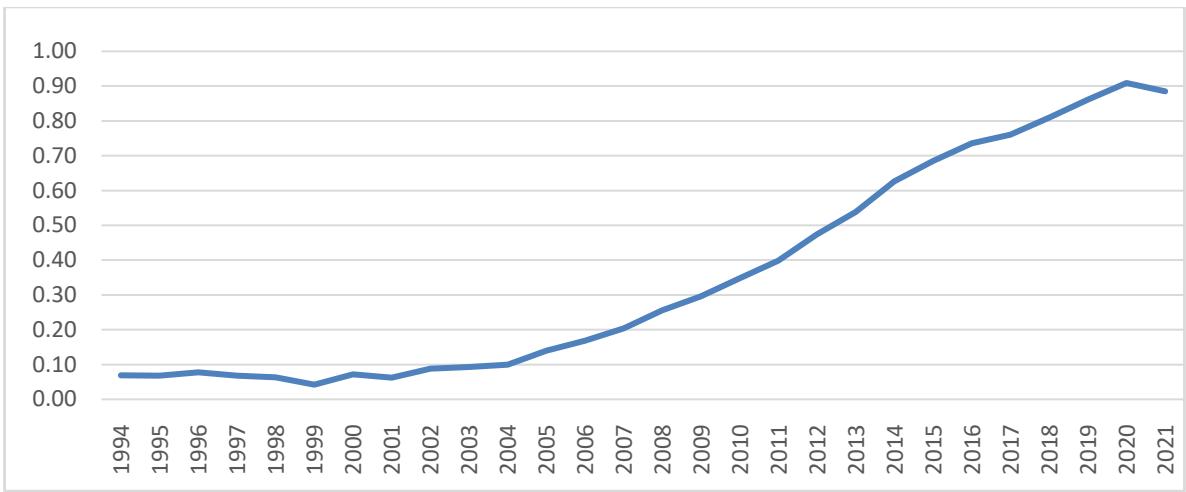Figure 1: Financial Inclusion Index for India Source: Prepared by authors. It is evident from Figure 1 that the FII values have shown a steady increase over the years. The initial years from 1994 to 2002 witnessed minimal growth, with FII values remaining relatively stagnant. However, from 2003 onward, there has been a noticeable upward trend, indicating a significant improvement in the FII values. The highest level of inclusion was observed in 2020, where the FII value approached 0.90. Although there was a slight decline in 2021, the overall trend suggests a consistent improvement in financial inclusion over the selected period. The FII values predominantly lie between 0.20 and 0.90, indicating a transition from low to high levels of financial inclusion in India over time. Additionally, an analysis of six key indicators for India has been conducted to explore the factors that impact the value of FII. This analysis provides important insights into the dynamics of access, usage and market penetration over the period. Figure 2 illustrates the analysis of these six FII indicators for India.  Number of bank branches per million population  No. of deposits a/c per 1000 pop  No. 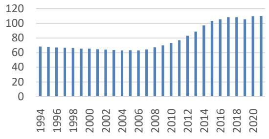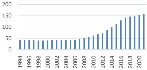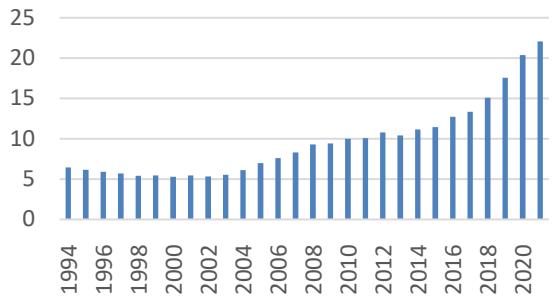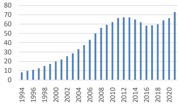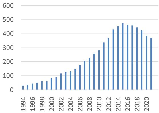of credit a/c per 1000 pop  Per capita deposit  Per capita credit CDR  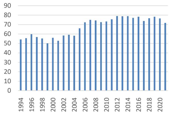Figure 2: Trend of Six Indicators of FII for India Source: Prepared by authors. Figure 2 provides a comprehensive view of financial inclusion in India by illustrating key indicators of financial inclusion over time. The availability of banking services, indicated by the number of bank branches per million population, initially shows a slight decline. This suggests a reduction in the physical banking infrastructure, which may be attributed to the growing reliance on digital banking solutions, reducing the need for traditional brick-and-mortar branches. However, the number of bank branches per million population increased rapidly after 2006. In terms of banking penetration, which is measured by the number of deposit accounts per 1,000 population, the graph reveals some initial fluctuations and a decline. However, as time progresses, the trend begins to stabilise and move upward, signifying an increase in access to banking services for a broader section of the population. This growing access is a positive indicator of enhanced financial inclusion. Credit penetration, represented by the number of credit accounts per 1,000 population, follows a similar pattern. The data shows fluctuations, but overall, India has seen growth in credit access over the years. This increase highlights the expanding availability of credit facilities, allowing more people to engage in economic activities that require borrowing, such as business ventures or personal investments. Per capita deposits have been steadily increasing, as shown by the upward trend in the graph. This rise reflects a greater capacity for saving among the Indian population, which is crucial for financial stability and long-term security. Similarly, per capita credit has also risen, indicating improved borrowing capacity, which supports both consumption and investment- key drivers of economic growth. Lastly, the credit-deposit ratio, which compares the total loans extended by banks to the total deposits, shows a consistent upward trend in India. This indicates that banks are extending credit in proportion to their deposits, reflecting a healthy and balanced financial system. Despite fluctuations in some indicators, the overall trend points toward greater financial inclusion, with improved access to both credit and deposit services, even as the physical banking infrastructure has declined. This highlights India's ongoing transition toward a more digital and inclusive financial environment. ### c) Independent Variables- Good Governance Indicators For the independent variables, the study considers the good governance indicators, which include the following: 1. Control of Corruption (CC): CC measures the extent to which public power is used for private gain, including both petty and grand corruption, as well as the capture of the state by elites and private interests. 2. Government Effectiveness (GE): GE assesses perceptions of public service quality, the independence of the civil service from political pressures, the quality of policy formulation and implementation and the credibility of government commitments. 3. Political Stability (PS): PS evaluates perceptions of political stability and the likelihood of politically motivated violence, including terrorism. 4. Regulatory Quality (RQ): RQ gauges the government's ability to formulate and implement policies and regulations that promote private sector development. 5. Rule of Law (ROL): ROL provides insight into confidence in and adherence to societal rules, focusing on contract enforcement, property rights, the police, the courts and the likelihood of crime and violence. 6. Voice and Accountability (VA): VA reflects perceptions of citizens' participation in selecting their government and includes freedom of expression, association and media freedom. These governance indicators are expressed in percentile ranks from 0 to 100, as shown in Figure 3, where higher ranks indicate stronger governance. For consistency, biannual data from 1996 to 2002 were converted to annual data using linear interpolation. 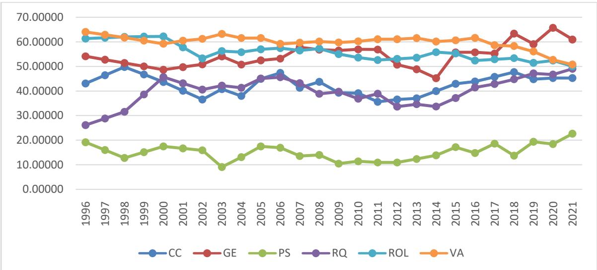 Figure 3: Trend of Good Governance Indicators Source: Prepared by authors. ### d) Control Variables In addition to taking good governance indicators as independent variables, this study also incorporates three control variables that are potentially relevant to financial inclusion. These control variables are GDP per capita, foreign direct investment (FDI) and inflation. These control variables are essential for ensuring the robustness of the analysis and for isolating the specific effects of good governance on financial inclusion. GDP per capita measures the average economic output per person. It is a critical indicator of economic development. A higher GDP per capita generally implies a higher standard of living, greater economic stability and increased access to resources. In the context of financial inclusion, a higher GDP per capita could lead to greater financial literacy, increased demand for financial services and more substantial investment in financial infrastructure. By including GDP per capita as a control variable, this study aims to account for the general level of economic development in India, which could influence the level of financial inclusion independently of governance factors. FDI represents the investment made by foreign entities into the domestic economy. It plays a significant role in economic growth by bringing in capital, technology and expertise. In the context of financial inclusion, FDI can stimulate economic activity, create jobs and increase income levels, all of which can lead to a greater need for and access to financial services. Additionally, FDI can encourage the development of financial institutions and infrastructure, thus promoting financial inclusion. By controlling for FDI, this study accounts for the influence of foreign investments on financial inclusion, ensuring that the effects of good governance are not conflated with the benefits brought by foreign capital. Inflation, the rate at which the general price level of goods and services rises, is another critical macroeconomic variable that can impact financial inclusion. High inflation can erode the value of money, reduce purchasing power and increase uncertainty in the economy. This could lead to a decrease in savings and investment, thereby affecting the demand for financial services. On the other hand, moderate inflation indicates the macroeconomic stability of an economy, which is often associated with economic growth and can lead to increased financial activity. By including inflation as a control variable, this study aims to isolate the impact of governance on financial inclusion from the effects of price level changes in the economy. By incorporating these control variables- GDP per capita, FDI, and inflation this study ensures a more comprehensive and accurate analysis of the relationship between good governance and financial inclusion in India. The inclusion of these variables allows for a clearer understanding of how governance specifically influences financial inclusion, beyond the general economic conditions and external investments that also play a role in this process. All the considered variables are used in their log form for further analysis. ## III. ESTIMATION TECHNIQUE ### a) Pre-Estimation Tests Before estimating the model, several pre-estimation tests are conducted to ensure the robustness and reliability of the selected econometric model. These tests help in understanding the characteristics of the data and verifying the appropriateness of the ARDL model for analysis. The first step involves examining the descriptive statistics of the variables to understand their fundamental properties, such as mean, standard deviation, skewness and kurtosis. This provides insights into the distributional characteristics of the data. Additionally, a correlation matrix is constructed to assess the degree of association between the variables, helping to identify potential multicollinearity issues that may affect the model's performance. Since time-series data is often characterised by trends and non-stationary behaviour, it is crucial to determine the stationarity of the variables before proceeding with model estimation. The order of integration of the variables, which refers to the number of times a series needs to be differenced to achieve stationarity, must be established. To Determine the Order of Integration, the Study Employs Two Widely used Unit Root Tests: The Augmented Dickey-Fuller (ADF) Test (Dickey & Fuller, 1979) to examine the presence of a unit root in the data and determine whether the series is stationary or requires differencing. Phillips-Perron (PP) Test (Phillips & Perron, 1988). This test extends the ADF test by adjusting for heteroskedasticity and autocorrelation, making it a robust alternative for detecting unit roots. Both tests are applied to each variable at levels and first differences to classify them as either stationary at level $[1(0)]$ or stationary after differencing $[1(1)]$. The ARDL model requires that variables be either $1$ (0) or $1$ (1), but not $1$ (2), ensuring that the model is appropriately specified. ### b) Estimation Test Once the stationarity tests confirm that the variables exhibit a mixed order of integration, some being I (0) and others I (1), the ARDL model can be appropriately specified. The ARDL approach to cointegration is particularly advantageous as it allows for the estimation of relationships among variables with different integration properties, making it a robust method for analysing both short-run and long-run dynamics. One of the key strengths of the ARDL model is its flexibility; it can be applied regardless of whether the variables are purely I (0), purely I (1), or a combination of both. This makes it a versatile tool for examining the long-run and short-run interactions between financial inclusion and governance indicators in India. The ARDL model, as specified in Equation (4), determines the optimal number of lags for the variables, facilitating an in-depth analysis of the long-term relationship between financial inclusion and good governance. $$ \begin{array}{l} \Delta l n F I I _ {t} = \alpha_ {0} + \lambda_ {1} l n F I I _ {t - 1} + \lambda_ {2} l n C C _ {t - 1} + \lambda_ {3} l n G E _ {t - 1} + \lambda_ {4} l n P S _ {t - 1} + \lambda_ {5} l n R Q _ {t - 1} + \lambda_ {6} l n R O L _ {t - 1} + \\\lambda_ {7} \ln V A _ {t - 1} + \lambda_ {8} \ln G D P P C _ {t - 1} + \lambda_ {9} \ln F D I _ {t - 1} + \lambda_ {1 0} \ln I N _ {t - 1} + \sum_ {i = 1} ^ {p - 1} \beta_ {1 j} \Delta \ln F I I _ {t - i} + \\\sum_ {j = 0} ^ {q _ {1} - 1} \boldsymbol{\beta} _ {2 j} \Delta \ln C C _ {t - j} + \sum_ {j = 0} ^ {q _ {2} - 1} \boldsymbol{\beta} _ {3 j} \Delta \ln G E _ {t - j} + \sum_ {j = 0} ^ {q _ {3} - 1} \boldsymbol{\beta} _ {4 j} \Delta \ln P S _ {t - j} + \sum_ {j = 0} ^ {q _ {4} - 1} \boldsymbol{\beta} _ {5 j} \Delta \ln R Q _ {t - j} + \sum_ {j = 0} ^ {q _ {5} - 1} \boldsymbol{\beta} _ {6 j} \Delta \ln R O L _ {t - j} + \\\sum_ {j = 0} ^ {q _ {6} - 1} \beta_ {7 j} \Delta l n V A _ {t - j} + \sum_ {j = 0} ^ {q _ {7} - 1} \beta_ {8 j} \Delta l n G D P P C _ {t - j} + \sum_ {j = 0} ^ {q _ {8} - 1} \beta_ {9 j} \Delta l n F D I _ {t - j} + \sum_ {j = 0} ^ {q _ {9} - 1} \beta_ {1 0 j} \Delta l n I N _ {t - j} + e _ {t} \tag{4} \\end{array} $$ In this model, $\Delta$ denotes the difference operator, $\alpha$ is a constant term and $\lambda_1 - \lambda_{10}$ and $\beta_{1} - \beta_{10}$ represent the long-term and short-term coefficients, respectively. The term $e$ is the stochastic error term. Equation (4) is considered to be cointegrated if there exists a long-term relationship among the variables InFII, InCC, InGE, InPS, InRQ, InROL, InVA, InGDPPC, InFDI and InIN. The estimation process begins by testing for cointegration, which essentially means determining whether the variables move together over the long term. Cointegration is established when the null hypothesis, which states that there is no long-term relationship $(H_0: \lambda_1 = \lambda_2 = \lambda_3 = \lambda_4 = \lambda_5 = \lambda_6 = \lambda_7 = \lambda_8 = \lambda_9 = \lambda_{10} = 0)$ is rejected. This rejection is based on the F-statistic derived from the model. If the F-statistic falls below the lower-bound critical value for I(0) at a 5 per cent significance level, the null hypothesis cannot be rejected, indicating no cointegration. Conversely, if the F-statistic exceeds the upper-bound critical value for I (1) at a 5 per cent significance level, the null hypothesis is rejected, confirming cointegration. If the F-statistic lies between the critical values, the test result is inconclusive. Once cointegration is confirmed, the next step is to estimate the Error-Correction Model (ECM). The ECM captures both short-run adjustments and the long-run equilibrium in response to any volatility in the variables, ensuring that the system eventually returns to equilibrium. This process is detailed in the following (5) equation. $$ \begin{array}{l} \Delta \ln F I I _ {t} = \alpha_ {0} + \sum_ {i = 1} ^ {p - 1} \beta_ {1 j} \Delta \ln F I I _ {t - i} + \sum_ {j = 0} ^ {q _ {1} - 1} \beta_ {2 j} \Delta \ln C C _ {t - j} + \sum_ {j = 0} ^ {q _ {2} - 1} \beta_ {3 j} \Delta \ln G E _ {t - j} + \sum_ {j = 0} ^ {q _ {3} - 1} \beta_ {4 j} \Delta \ln P S _ {t - j} + \\\sum_ {j = 0} ^ {q _ {4} - 1} \beta_ {5 j} \Delta l n R Q _ {t - j} + \sum_ {j = 0} ^ {q _ {5} - 1} \beta_ {6 j} \Delta l n R O L _ {t - j} + \sum_ {j = 0} ^ {q _ {6} - 1} \beta_ {7 j} \Delta l n V A _ {t - j} + \sum_ {j = 0} ^ {q _ {7} - 1} \beta_ {8 j} \Delta l n G D P P C _ {t - j} + \\\sum_ {j = 0} ^ {q _ {8} - 1} \boldsymbol{\beta} _ {9 j} \Delta \ln F D I _ {t - j} + \sum_ {j = 0} ^ {q 9 - 1} \boldsymbol{\beta} _ {1 0 j} \Delta \ln I N _ {t - j} + \delta E C T _ {t - 1} + \varepsilon_ {t} \tag{5} \\end{array} $$ In the equation (5), $ECT_{t-1}$ represents the lagged error correction term derived from the cointegrating equation, with its coefficient $\delta$ indicating the speed of adjustment. This coefficient measures how quickly the system returns to its long-term equilibrium after short-term disturbances. For stability, the value of $\delta$ should be significant and it should lie between 0 and -1. ### c) Post-Estimation Tests After estimating the model, several post-estimation tests are conducted to assess the robustness and reliability of the results. These diagnostic tests help ensure the validity and stability of the estimated model. To detect potential econometric issues, the Breusch-Pagan-Godfrey test is used to check for heteroskedasticity, while the Breusch-Godfrey LM test assesses autocorrelation in the residuals. The Jarque-Bera test is employed to examine whether the residuals follow a normal distribution. Additionally, model stability is verified using the Ramsey RESET test, along with the CUSUM and CUSUM of squares tests, which evaluate the structural stability of the estimated parameters over time. Furthermore, to validate the long-run relationships obtained through the ARDL model, the study employs the Fully Modified Ordinary Least Squares (FMOLS) method (Phillips and Hansen, 1990) and Canonical Cointegration Regression (CCR) method (Park, 1992). These techniques provide robust estimates by addressing potential endogeneity and serial correlation issues, thereby enhancing the credibility of the long-run results. ## IV. RESULTS AND DISCUSSIONS This section begins with an overview of the summary statistics, which include descriptive statistics and a correlation matrix, as given in Table 3. Table 3: Descriptive Statistics and Correlation Matrix of Selected Variables <table><tr><td></td><td>InFII</td><td>InCC</td><td>InGE</td><td>InPS</td><td>InRQ</td><td>InROL</td><td>InVA</td><td>InGDPPC</td><td>InFDI</td><td>InIN</td></tr><tr><td colspan="11">Descriptive Statistics</td></tr><tr><td>Mean</td><td>-1.42</td><td>3.74</td><td>3.99</td><td>2.68</td><td>3.67</td><td>4.02</td><td>4.09</td><td>7.03</td><td>0.27</td><td>1.64</td></tr><tr><td>Median</td><td>-1.29</td><td>3.76</td><td>3.99</td><td>2.70</td><td>3.71</td><td>4.01</td><td>4.10</td><td>7.02</td><td>0.41</td><td>1.73</td></tr><tr><td>Max.</td><td>-0.09</td><td>3.90</td><td>4.18</td><td>3.11</td><td>3.89</td><td>4.13</td><td>4.15</td><td>7.58</td><td>1.28</td><td>2.35</td></tr><tr><td>Mini.</td><td>-3.17</td><td>3.57</td><td>3.81</td><td>2.20</td><td>3.26</td><td>3.91</td><td>3.92</td><td>6.47</td><td>-0.74</td><td>0.82</td></tr><tr><td>S. D.</td><td>1.03</td><td>0.09</td><td>0.08</td><td>0.22</td><td>0.15</td><td>0.06</td><td>0.05</td><td>0.36</td><td>0.52</td><td>0.44</td></tr><tr><td>Ske.</td><td>-0.14</td><td>-0.29</td><td>0.23</td><td>-0.26</td><td>-0.94</td><td>0.46</td><td>-1.87</td><td>0.03</td><td>-0.24</td><td>-0.20</td></tr><tr><td>Kur.</td><td>1.50</td><td>1.99</td><td>2.87</td><td>2.41</td><td>3.36</td><td>2.22</td><td>6.51</td><td>1.65</td><td>2.14</td><td>1.77</td></tr><tr><td>J-Bera</td><td>2.52</td><td>1.47</td><td>0.26</td><td>0.67</td><td>4.04</td><td>1.57</td><td>28.58</td><td>1.96</td><td>1.05</td><td>1.80</td></tr><tr><td>Prob.</td><td>0.28</td><td>0.47</td><td>0.87</td><td>0.71</td><td>0.13</td><td>0.45</td><td>0.00</td><td>0.37</td><td>0.59</td><td>0.40</td></tr></table> Correlation Matrix <table><tr><td>InFII</td><td>1.00</td><td></td><td></td><td></td><td></td><td></td><td></td><td></td><td></td></tr><tr><td>InCC</td><td>-0.05</td><td>1.00</td><td></td><td></td><td></td><td></td><td></td><td></td><td></td></tr><tr><td>InGE</td><td>0.52</td><td>0.30</td><td>1.00</td><td></td><td></td><td></td><td></td><td></td><td></td></tr><tr><td>InPS</td><td>0.09</td><td>0.52</td><td>0.17</td><td>1.00</td><td></td><td></td><td></td><td></td><td></td></tr><tr><td>InRQ</td><td>0.29</td><td>0.14</td><td>0.40</td><td>0.24</td><td>1.00</td><td></td><td></td><td></td><td></td></tr><tr><td>InROL</td><td>-0.83</td><td>0.34</td><td>-0.50</td><td>0.00</td><td>-0.46</td><td>1.00</td><td></td><td></td><td></td></tr><tr><td>InVA</td><td>-0.55</td><td>-0.29</td><td>-0.59</td><td>-0.50</td><td>-0.62</td><td>0.53</td><td>1.00</td><td></td><td></td></tr><tr><td>InGDPPC</td><td>0.97</td><td>0.01</td><td>0.54</td><td>0.14</td><td>0.43</td><td>-0.84</td><td>-0.63</td><td>1.00</td><td></td></tr><tr><td>InFDI</td><td>0.73</td><td>-0.13</td><td>0.48</td><td>-0.02</td><td>0.29</td><td>-0.58</td><td>-0.39</td><td>0.67</td><td>1.00</td></tr><tr><td>LnIN</td><td>-0.07</td><td>-0.14</td><td>0.14</td><td>-0.28</td><td>-0.27</td><td>0.03</td><td>0.02</td><td>-0.17</td><td>0.15</td></tr></table> Table 3 provides insights into the distribution and relationships among the variables studied. The InFII displays significant variability, with the mean indicating generally low financial inclusion. Governance indicators, such as InCC and InGE, show less variability, reflecting their relative stability over time. Correlation analysis reveals a strong positive relationship between financial inclusion and both InGDPPC and InFDI, underscoring the importance of economic factors in promoting financial inclusion. However, some governance indicators, like InROL and InVA, are negatively correlated with financial inclusion, suggesting a complex relationship that may not always align with higher levels of financial inclusion. The results indicate that while economic growth and foreign investment are crucial for financial inclusion, the influence of governance indicators is more nuanced, warranting further exploration to fully understand their impact. The stationarity of the variables in the study is tested by the Augmented Dickey-Fuller (ADF) and Phillips-Perron (PP) tests. The results of stationarity are given in Table 4. Table 4: Results of the Stationarity Test <table><tr><td colspan="5">Augmented Dickey-Fuller</td><td colspan="4">Phillips-Perron</td></tr><tr><td>Variable</td><td colspan="2">Level</td><td colspan="2">First Difference</td><td colspan="2">Level</td><td colspan="2">First Difference</td></tr><tr><td></td><td>Intercept &amp; Trend</td><td>Intercept</td><td>Intercept &amp; Trend</td><td>Intercept</td><td>Intercept &amp; Trend</td><td>Intercept</td><td>Intercept &amp; Trend</td><td></td></tr><tr><td>InFII</td><td>-3.74**</td><td>0.36</td><td>-5.05***</td><td>-3.10</td><td>-0.19</td><td>-2.78</td><td>-6.17***</td><td>-6.00***</td></tr><tr><td>InCC</td><td>-2.07</td><td>-2.01</td><td>-5.38***</td><td>-5.39***</td><td>-2.23</td><td>-2.15</td><td>-5.36***</td><td>-5.41***</td></tr><tr><td>InGE</td><td>-1.95</td><td>-2.81</td><td>-6.41***</td><td>-6.39***</td><td>-2.00</td><td>-2.85</td><td>-6.39***</td><td>-6.39***</td></tr><tr><td>InPS</td><td>-2.66*</td><td>-2.72</td><td>-6.22***</td><td>-6.37***</td><td>-2.65*</td><td>-2.67</td><td>-6.78***</td><td>-8.77***</td></tr><tr><td>InRQ</td><td>-2.62</td><td>-2.39</td><td>-3.78***</td><td>-3.69**</td><td>-2.16</td><td>-2.46</td><td>-3.75***</td><td>-3.66**</td></tr><tr><td>InROL</td><td>-1.20</td><td>-3.76**</td><td>-4.85***</td><td>-4.73***</td><td>-1.03</td><td>-2.87</td><td>-5.07***</td><td>-4.90***</td></tr><tr><td>InVA</td><td>1.04</td><td>0.15</td><td>-3.66**</td><td>-4.01**</td><td>0.67</td><td>-0.30</td><td>-3.71**</td><td>-3.99**</td></tr><tr><td>InGDPPC</td><td>-0.32</td><td>-2.57</td><td>-4.78***</td><td>-4.71***</td><td>-0.31</td><td>-2.28</td><td>-4.78***</td><td>-4.71***</td></tr><tr><td>InFDI</td><td>-2.08</td><td>-2.23</td><td>-5.12***</td><td>-5.04***</td><td>-2.08</td><td>-2.23</td><td>-5.12***</td><td>-5.04***</td></tr><tr><td>InIN</td><td>-2.21</td><td>-2.02</td><td>-5.07***</td><td>-5.05***</td><td>-2.24</td><td>-2.05</td><td>-5.07***</td><td>-5.05***</td></tr></table> The results of Table 4 indicate that for most variables, including the InFII, InCC and InGE, the null hypothesis of a unit root is rejected at the first difference level, indicating stationarity after differencing. Specifically, variables such as InFII, InCC and InGE are found to be stationary in their first differences under both the intercept and trend specifications. The variable InPS is stationary at the level under the intercept specification according to both tests. Other variables, like InRQ and InROL, also show stationarity after differencing, though some, like InVA, are stationary only under certain test specifications. Similarly, InGDPPC, InFDI and InIN are stationary in their first differences. These findings suggest that the variables are integrated of order I(0) and I(1), supporting the use of the ARDL model that accommodates both I(0) and I(1) processes, for further analysis of the relationship between governance and financial inclusion. The results of the optimal lag selection criteria are given in Table 5. Table 5: Lag Order Selection Criteria in Vector Autoregressive (VAR) Model <table><tr><td>Lag</td><td>LogL</td><td>LR</td><td>FER</td><td>AIC</td><td>SC</td><td>HQ</td></tr><tr><td>0</td><td>203.94</td><td>NA</td><td>8.65e-20</td><td>-15.51</td><td>-15.02</td><td>-15.38</td></tr><tr><td>1</td><td>422.88</td><td>245.20</td><td>1.21e-23</td><td>-25.03*</td><td>-19.66</td><td>-23.54</td></tr></table> Table 5 indicates that optimal lag selection criteria, including AIC, SC and HQ, favour the inclusion of one lag in the VAR model. Consequently, the VAR model with one lag is deemed optimal based on the selection criteria. The results of the bound test for cointegration are presented in Table 6. Table 6: Results of Bound Test <table><tr><td>Test Statistic</td><td>Value</td><td>Signif.</td><td>I(0)</td><td>I(1)</td></tr><tr><td>F- Statistic</td><td>11.08</td><td>10%</td><td>1.8</td><td>2.8</td></tr><tr><td>K</td><td>9</td><td>5%</td><td>2.04</td><td>2.08</td></tr><tr><td></td><td></td><td>2.5%</td><td>2.24</td><td>3.35</td></tr><tr><td></td><td></td><td>1%</td><td>2.5</td><td>3.68</td></tr></table> The results of Table 6 show an F-statistic value of 11.08, which exceeds the critical values for upper limit I(1) at various significance levels, indicating a significant cointegrating relationship among the variables at the 1 per cent level of significance. This suggests a long-term equilibrium relationship among the series, confirming cointegration. The results of long-run coefficients and the error correction term are presented in Table 7. Table 7: Results for Long-Run Coefficients and Error Correction Term <table><tr><td colspan="4">Dependent variable- FII</td></tr><tr><td>Variable</td><td>Coefficient</td><td>Std. Error</td><td>t-statistic</td></tr><tr><td colspan="4">Normalized Long-run Coefficients</td></tr><tr><td>InCC</td><td>-1.22</td><td>0.43</td><td>-2.80**</td></tr><tr><td>InGE</td><td>0.15</td><td>0.29</td><td>0.53</td></tr><tr><td>InPS</td><td>0.26</td><td>0.15</td><td>1.74</td></tr><tr><td>InRQ</td><td>-0.81</td><td>0.17</td><td>-4.61*</td></tr><tr><td>InROL</td><td>0.50</td><td>0.75</td><td>0.66</td></tr><tr><td>InVA</td><td>0.42</td><td>0.68</td><td>0.61</td></tr><tr><td>InGDPPC</td><td>2.81</td><td>0.13</td><td>21.30*</td></tr><tr><td>InFDI</td><td>0.20</td><td>0.05</td><td>3.94*</td></tr><tr><td>InIN</td><td>0.08</td><td>0.04</td><td>1.96***</td></tr><tr><td>C</td><td>-19.02</td><td>5.82</td><td>-3.26**</td></tr><tr><td colspan="4">Error Correction Model</td></tr><tr><td>D(InCC)</td><td>-0.60</td><td>0.13</td><td>-4.42*</td></tr><tr><td>D(InPS)</td><td>0.04</td><td>0.04</td><td>0.98</td></tr><tr><td>D(InRQ)</td><td>-0.54</td><td>0.12</td><td>-4.25*</td></tr><tr><td>D(InVA)</td><td>-1.45</td><td>0.45</td><td>-3.18**</td></tr><tr><td>D(InGDPPC)</td><td>3.34</td><td>0.22</td><td>15.15*</td></tr><tr><td>D(InFDI)</td><td>0.22</td><td>0.02</td><td>7.71*</td></tr><tr><td>ECTt-1</td><td>-0.54</td><td>0.09</td><td>-6.00*</td></tr></table> Table 7 shows the results of the long-run coefficients and the error correction term with the FII as the dependent variable. In the long-run analysis, several variables significantly affect financial inclusion. Notably, the coefficient for InCC is -1.22 with a t-statistic of -2.80, indicating a significant negative impact on financial inclusion. This suggests that better control of corruption is associated with improved financial inclusion. The InRQ also shows a significant negative effect with a coefficient of -0.81 and a t-statistic of -4.61, implying that a stronger rule of law may be linked to lower financial inclusion, possibly due to the complexity or barriers created by stringent regulations. Conversely, the coefficients for InGE, InPS and InROL are not statistically significant, indicating that these factors do not have a significant long-term impact on financial inclusion in this model. However, InFDI and InGDPPC show significant positive effects on financial inclusion in the long run. In the short run, the coefficient of the error correction term $(ECT_{t - 1})$ is -0.54 with a highly significant t-statistic of -6.00, indicating rapid adjustment of the model to restore equilibrium after short-term deviations, reflecting strong and efficient correction mechanisms towards long-term financial inclusion. The coefficients for changes in Control of Corruption, Rule of Law and Political Stability also show significant short-term effects on financial inclusion, highlighting their roles in adjusting short-term fluctuations. However, InFDI and InGDPPC show significant positive effects on financial inclusion in the short run. Overall, the results suggest that while some governance indicators, like Control of Corruption and Rule of Law, have significant long-term impacts on financial inclusion, others, such as Government Effectiveness and Political Stability, do not. However, the economic variables InFDI and InGDPPC show significant positive effects on financial inclusion in the short run. The model effectively corrects deviations, ensuring that financial inclusion moves towards a long-term equilibrium. The results of model diagnostic tests are given in Table 8. Table 8: Results of Model Diagnostic Tests <table><tr><td>Test</td><td>Test Statistic</td><td>Conclusion</td></tr><tr><td>Jarque-Bera Test for Normality</td><td>JB = 0.84 (0.65)</td><td>Residuals are normally distributed</td></tr><tr><td>Breusch-Godfrey LM Test for Serial Correlation</td><td>F = 3.26 (0.10)</td><td>No serial correlation in residuals</td></tr><tr><td>Breusch-Pagan-Godfrey Test for Heteroscedasticity</td><td>F = 1.30 (0.36)</td><td>No heteroscedasticity in residuals</td></tr><tr><td>Ramsey RESET Test</td><td>F = 6.71 (0.08)</td><td>The model is correctly specified</td></tr></table> The results given in Table 8 indicate that the residuals are normally distributed, as evidenced by the Jarque-Bera test. The Breusch-Godfrey LM test for serial correlation confirms no serial correlation in the residuals, suggesting that they are independent over time. The Breusch-Pagan-Godfrey test for heteroscedasticity shows no evidence of heteroscedasticity, meaning that the variance of the residuals remains consistent across different levels of the independent variables. The Ramsey RESET test indicates that the model is correctly specified, affirming that the functional form of the model is appropriate. These results suggest that the model is reliable, with no major issues in its residuals and that the estimates produced are likely valid. The results of the CUSUM and CUSUM of Squares tests are given in Figure 4.  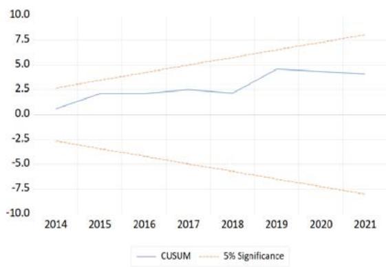Source: Constructed by authors.  Figure 4: Result of the CUSUM and CUSUM Square Test The CUSUM test shows that the line remains within the $5\%$ significance boundaries throughout the period from 2014 to 2021, indicating that the model's coefficients are stable over time. This stability suggests that the relationships between the variables have not significantly changed during the observed period. Similarly, the CUSUM of Squares test indicates that the variance of the residuals is stable over this period, implying that the model is homoscedastic, with constant variance in its errors, a desirable property in time series analysis. The model is re-estimated by FMOLS and CCR methods, addressing endogeneity and serial correlation issues to validate the ARDL model's long-term outcomes. The results of these methods are given in Table 9. Table 9: Results of ARDL, FMOLS and CCR Methods <table><tr><td colspan="4">Dependent variable- FII</td></tr><tr><td>Variable</td><td>ARDL</td><td>FMOLS</td><td>CCR</td></tr><tr><td>InCC</td><td>-2.80**</td><td>-2.11**</td><td>-1.46</td></tr><tr><td>InGE</td><td>0.53</td><td>0.76</td><td>0.44</td></tr><tr><td>InPS</td><td>1.74</td><td>2.03**</td><td>2.09**</td></tr><tr><td>InRQ</td><td>-4.61*</td><td>-0.844*</td><td>-5.04*</td></tr><tr><td>InROL</td><td>0.66</td><td>0.44</td><td>-5.04*</td></tr><tr><td>InVA</td><td>0.61</td><td>1.58</td><td>1.10</td></tr><tr><td>InGDPPC</td><td>21.30*</td><td>22.66*</td><td>15.68*</td></tr><tr><td>InFDI</td><td>3.94*</td><td>3.66*</td><td>2.82**</td></tr><tr><td>InIN</td><td>1.96***</td><td>2.83**</td><td>2.27**</td></tr><tr><td>C</td><td>-3.26**</td><td>-4.28*</td><td>-2.74**</td></tr></table> The results given in Table 9 indicate that Control of Corruption shows a consistent negative impact on FII, with statistically significant coefficients in both the ARDL and FMOLS methods, though this effect weakens in the CCR method. Government Effectiveness does not demonstrate a strong influence on FII, as the coefficients across all methods are positive but not statistically significant. Political Stability, however, positively correlates with FII, with significant coefficients in the FMOLS and CCR methods. Regulatory Quality exhibits a negative relationship with FII across all methods, with statistically significant results, particularly in the ARDL and CCR methods. The impact of the Rule of Law varies, with the CCR method showing a significant negative effect, contrasting with the non-significant results in ARDL and FMOLS. Voice and Accountability do not significantly affect FII in any method. Lagged GDP per capita consistently shows a strong positive relationship with current FII across all methods, indicating a momentum effect. Foreign Direct Investment also has a positive and significant impact across all methods. Inflation is positively associated with FII, with significant coefficients in the ARDL, FMOLS and CCR methods. Results show that estimates from these techniques closely align in signs and magnitudes with ARDL model results, ensuring the robustness of the estimates. Consistency across estimation techniques strengthens confidence in the reliability of the ARDL model. The results indicate that financial inclusion in the studied context is strongly influenced by economic factors such as GDP per capita and foreign direct investment, which are both positively correlated with financial inclusion. However, the impact of governance indicators is more complex. While better control of corruption appears to enhance financial inclusion, other governance factors like the rule of law may have a negative or nuanced effect. ## V. CONCLUSION The study offers a nuanced exploration of the impact of good governance on financial inclusion in India, integrating a range of econometric methods to provide a comprehensive analysis of both long-term and short-term relationships. The descriptive statistics reveal substantial variability in the Financial Inclusion Index, highlighting generally low levels of financial inclusion across the board. In contrast, governance indicators such as Control of Corruption and Government Effectiveness show relative stability, reflecting their consistent nature over time. The correlation analysis underscores a strong positive relationship between financial inclusion and economic factors, specifically GDP per capita and Foreign Direct Investment, indicating that economic growth and foreign investment are crucial drivers of financial inclusion. However, some governance indicators, such as Rule of Law and Voice and Accountability, exhibit negative correlations with financial inclusion, suggesting that their impact is more complex and may not always align with increased financial inclusion. The study tested the stationarity of the variables through the Augmented Dickey-Fuller and Phillips-Perron tests. The results indicate that the variables are integrated of order I(0) and I (1). This finding supports the application of the ARDL model that can handle variables which are both I(0) and I (1). Model selection criteria, including AIC, SC and HQ, suggest that a VAR model with one lag is optimal, as evidenced by improved LogL and LR statistics. The bound test for cointegration reveals a significant cointegrating relationship among the variables, indicating a long-term equilibrium. The long-run analysis demonstrates that Control of Corruption and the Rule of Law have significant negative effects on financial inclusion, while FDI and GDPPC have a significant positive impact. The short-run analysis shows that deviations from equilibrium are corrected rapidly, with significant short-term effects from governance indicators like Control of Corruption and Rule of Law. Similarly, the economic variables InFDI and InGDPPC show significant positive effects on financial inclusion in the short run. Model diagnostics affirm the reliability of the results. Tests for normality, serial correlation, heteroscedasticity and model specification suggest that the residuals are normally distributed, free of serial correlation and heteroscedasticity and that the model is correctly specified. The stability of the model is further supported by the CUSUM tests, indicating that the model's coefficients and residual variance remain stable over the observed period. Robustness checks using ARDL, FMOLS and CCR methods reveal the robustness of the models. In conclusion, this study provides a comprehensive analysis of the interplay between good governance and financial inclusion in India, using robust econometric methods to uncover both long- and short-term dynamics. While economic factors like GDP per capita and FDI significantly enhance financial inclusion, governance indicators such as Control of Corruption and Rule of Law exhibit more complex, sometimes negative effects. The findings highlight the nuanced role of governance in financial inclusion, with both equilibrium corrections and stability tests confirming the model's reliability. Overall, the study underscores the importance of balancing economic growth and governance reforms to drive inclusive financial development. Finally, further research is needed to delve into specific mechanisms through which governance affects financial inclusion, providing deeper insights for targeted policy interventions. Implementing a balanced approach that integrates economic and governance factors will be crucial for advancing financial inclusion and promoting broader economic development in India Authors' Contributions All authors contributed equally to this research. Professor C. R. Bishnoi conceived the idea and provided guidance, while Ayushi Vashistha and Ashi Jain developed the conceptual framework, designed the methodology and co-authored the manuscript with his input. Conflict of Interest Fundings Acknowledgement The authors did not receive any financial support for the research, authorship or publication of this article.

Generating HTML Viewer...

References

16 Cites in Article
David Dickey,Wayne Fuller (1979). Distribution of the Estimators for Autoregressive Time Series with a Unit Root.
Tarek Eldomiaty,Rasha Hammam,Rawan El Bakry (2020). Institutional determinants of financial inclusion: evidence from world economies.
R Goldsmith (1969). Financial structure and development.
Arindam Laha (2015). Association between Governance and Human Development in South Asia.
Sanjaya Lenka,Ruchi Sharma (2017). Does Financial Inclusion Spur Economic Growth in India?.
R Mckinnon (1973). Money and capital in economic development.
Joon Park (1992). Canonical Cointegrating Regressions.
Cyn-Young Park,Rogelio Mercado (2017). FINANCIAL INCLUSION, POVERTY, AND INCOME INEQUALITY.
M Pesaran,Yongcheol Shin,Richard Smith (2001). Bounds testing approaches to the analysis of level relationships.
Peter Phillips,Bruce Hansen (1990). Statistical Inference in Instrumental Variables Regression with I(1) Processes.
P Phillips,P Perron (1988). Testing for a unit root in time series regression.
C Rangarajan (2008). Report of the Committee on Financial Inclusion.
(2005). Annual Policy Statement for the year 2005-06.
M Sarma (2008). Index of Financial inclusion.
Joseph Schumpeter (1911). The Theory of Economic Development.
Quanda Zhang,Alberto Posso (2017). Thinking Inside the Box: A Closer Look at Financial Inclusion and Household Income.
No ethics committee approval was required for this article type.
Data Availability
Not applicable for this article.
How to Cite This Article
Dr. C.R. Bishnoi. 2026. \u201cImpact of Good Governance on Financial Inclusion in India: Evidence from the ARDL Bounds Testing Approach\u201d. Global Journal of Management and Business Research - B: Economic & Commerce GJMBR-B Volume 25 (GJMBR Volume 25 Issue B2): .
Explore published articles in an immersive Augmented Reality environment. Our platform converts research papers into interactive 3D books, allowing readers to view and interact with content using AR and VR compatible devices.
Your published article is automatically converted into a realistic 3D book. Flip through pages and read research papers in a more engaging and interactive format.
Our website is actively being updated, and changes may occur frequently. Please clear your browser cache if needed. For feedback or error reporting, please email [email protected]
Thank you for connecting with us. We will respond to you shortly.