Renormalized Lambert–W Cascade and Finite-Time Amplification and Blowup for reconstructed b Dynamics on T^3 for the 3D Navier Stokes Equations

Terry Moschandreou

doi:10.34257/GJSFRF277130

1. Introduction and organization

Papers explicitly stating and showing that there are finite time singularities of the 3D incompressible Navier Stokes equations were not found in my literature search at the time of the published work in ^[1] and before it’s inception. There is the famous result of Terence Tao in ^[3] for a finite time blowup of the fluid equations but for an averaged NS equation. Going back to 2021 Moschandreou ^[4] showed that there are no-finite time singularities but left open the possibility of finite time blowup on sets of measure zero in $T^3$ (see also ^[5]). Singular solution behaviour was determined for the Euler and related partial differential equations in ^[6], ^[7] and ^[8]. Recently the existence of a nonsmooth periodic attractor is shown in ^[9]. Critical and important findings among papers in the theory of Navier Stokes equations span the years (1934-1984) and are ^[10],^[11], ^[12] and ^[13]. Important references in differential equations theory are found in ^[14],^[15],^[16],^[17] and a strong PDE source textbook is found in ^[18]. Next a solid coverage of vorticity and Incompressible Navier Stokes theory is found in ^[19]. Excellent sources on the Navier Stokes problem can be found in ^[20], ^[21],^[22], ^[23] and ^[24]. A compendium on the LambertW function and it’s theory is found in ^[25]. And finally a very good reference in functional analysis and in particular on the Fredholm alternative and Fredholm compatability theory as used can be located here^[26] The analysis is organized around four linked structures: the distinguished phase $\theta=t-z$ ; the real renormalized Lambert map $\Delta\mapsto1+W_0(-e^{-1-\Delta})$ ; the characteristic invariant that transfers branch-distance collapse to amplification of $b_3$ ; and the corrected extended $b_3$ equation with periodic velocity reconstruction. The finite-depth cascade and finite-time characteristic proofs are presented first. The later sections retain the essential full- $b_3$ PDE reconstruction, comparison, trapping, and terminal closure arguments while suppressing duplicate derivations and exploratory restatements.

2. The Renormalized Lambert Cascade, Geometric Reconstruction, and Finite-Time Amplification Mechanism

The purpose of this paper is to present in condensed form the principal mathematical architecture developed first in a longer construction which I used to simplify with full import to the present paper. For example some steps were implicit but have been worked out thoroughly filling in completely any gaps in the flow of the reading of this particular work. The central mechanism begins with a renormalized Lambert– $W$ cascade, passes through a distinguished scalar product variable

and culminates in a characteristic regime in which the Lambert-generated logarithmic coefficient produces a positive quadratic amplification term. As stated in the conclusion of ^[1] this leads to:
”In particular, the analysis shows that singular behavior is associated with the branch structure of the Lambert W function rather than unbounded growth of the solution itself at time $t_1<t_2$ . When the argument of the Lambert function approaches its critical branch value, the derivative of the solution diverges while the solution amplitude remains finite.” ^[1]
Further in the conclusion there it states explicitly: ”However there is a $\|b\|^2$ term which leads to blowup in derivatives as shown at $t=t_1$ and for $t=t_2(t_2>t_1)$ it was proven analytically and numerically that there is finite time amplitude blowup in the solution $b_3$ ”.

The analysis is carried out on the periodic domain

with velocity

A central point of the construction is that $b_3$ is not introduced merely as an auxiliary scalar. It remains the exact physical product

in the reconstructed velocity field. The scalar characteristic analysis and the geometric velocity reconstruction are therefore linked through an identity rather than through an asymptotic identification.

The reduced paper retains five principal structures:

The purpose of this introduction is to display this architecture before the proofs are developed in detail.

2.1. Historical symmetric precursor and the active reconstruction

An earlier symmetric stage of the construction used a common transverse profile

At that level,

so that

This symmetric representation remains useful for understanding the origin of several scalar formulas and preterminal periodic constructions. However, it is not the active terminal reconstruction used in the final analysis.

The active variables are instead

Thus

holds identically, whereas $u_y$ and $u_z$ are no longer assumed to coincide.

The two transverse components acquire different roles:

This distinction is fundamental to the presentation.

2.2. Renormalized Lambert– $W$ cascade

The scalar branch variable is generated by the principal real branch $W_0$ . Let

denote the initial branch distance and define

The terminal Lambert regime corresponds to

The local branch-point expansion is

Consequently, at every fixed finite depth $k$ ,

The distinguished terminal quantity will be denoted

Its logarithmic derivative is

When the branch distance is represented by a terminal coordinate $s$ for which

one obtains

Thus the renormalized cascade produces two simultaneous effects:

At the frequently used finite depth $k=3$ ,

It is essential to distinguish the branch variable $Q_N$ from the physical transverse velocity components. In the active reconstruction,

Rather,

The role of $Q_N$ is to generate $\Gamma_N$ , which enters the $b_3$ -equation. The physical velocity behavior is determined independently by the geometric reconstruction.

2.3. Distinguished phase $\theta=t-z$

The terminal analysis is organized around

After locating the distinguished branch position $\theta_{*,N}$ , define

Along the reduced characteristic for which

one obtains

This elementary identity becomes the trapping law.

If the terminal region is entered with

then

Hence

Thus the characteristic is driven toward the Lambert endpoint once the amplitude has crossed the threshold $b>1$ .

2.4. The corrected extended $b_3$ -equation

With

define the horizontal differential operator

and the transport operator

The corrected extended amplitude equation can be written

where

Equivalently, before the final compression of the reconstruction terms, one may write

Along a characteristic,

and therefore

The additional terms are not discarded. Their role is measured relative to the positive source.

Define

If

then

Hence

On the positive branch,

so

and consequently

This is the Riccati-type inequality that drives the terminal growth.

The logical reduction is therefore

Thus the reconstruction error is used explicitly in obtaining the quadratic lower bound.

2.5. The explicit reconstruction error

At an intermediate stage of the periodic reconstruction, the additional terms can be collected as

The terminal objective is

Equivalently,

A normalized estimate of the form

with

reduces the problem to weighted reconstruction bounds.

When

and

the first three normalized terms vanish.

For the remaining term, the terminal derivative estimate

gives

The comparison argument provides

and hence

Therefore

Consequently, for every fixed

one eventually has

and hence

This estimate is the bridge from the full extended PDE to the scalar terminal comparison.

2.6. Release-layer and square-root-core estimates

The terminal reconstruction naturally separates into a release layer and a deeper square-root core.

In the release layer,

In the square-root core,

Both estimates vanish as

Thus

and the geometric transition into the terminal square-root regime does not destroy the positive Lambert-generated quadratic term.

Rather, the error becomes progressively smaller relative to that term.

2.7. Finite-depth trapping and amplification

The two fundamental terminal inequalities are

and

For finite cascade depth $k$ ,

Since

one obtains

For $b>1$ ,

and therefore

Integration gives

Consequently,

At $k=3$ ,

The remaining physical characteristic time is finite because

The lower power-law bound gives

and hence

Thus

with

The same result can be expressed directly in terms of $Q_N$ . In the large-amplitude terminal regime,

Integration from a terminal-entry point

gives

Hence

The feedback mechanism is therefore

2.8. Square-root velocity geometry

The terminal geometric specialization begins with

Using

gives

and therefore

Thus

on the selected real branch.

Moreover,

Since

one obtains

Thus the square-root behavior follows directly from the geometric constraint and the exact product identity $b=u_xu_y$ .

2.9. Periodic realization through $\chi(x)$

On $\mathbb{T}^3$ , the local coordinate $x$ is replaced near a selected periodic zero by a smooth periodic function $\chi(x)$ . The active relation becomes

or equivalently

Therefore

The exact ratio is

Suppose $\chi$ has a simple zero and

Then

If

then

At $k=3$ ,

and hence

Consequently,

The singular behavior is therefore anisotropic.

2.10. Ordinary spatial distance and the $\mathcal{J}_3$ scaling

A convenient periodic choice is

Set

Near a distinguished zero, let

Because $\chi$ has a simple zero,

so

For the $k=3$ scaling

one obtains

and

The exponent identities

and

imply simultaneously

and

In particular,

Thus the divergence of $u_x$ is weaker than the reciprocal vanishing scale $1/\vert \chi\vert$ , and the identity

remains completely consistent with

For

reality of

requires

Near a simple zero of $\sin(x-x_*)$ , one may therefore select a one-sided interval

on which

Either real square-root branch

may be selected, with the corresponding sign of

2.11. Exact continuity and reconstruction of $u_z$

The square-root law determines $A=u_y$ , but it does not prescribe $C=u_z$ .

Exact incompressibility requires

Thus

Differentiating

gives

and

Hence

Therefore

In the distinguished terminal core,

one has

Since

continuity becomes

Using

this simplifies to

If

and

then

For $k=3$ in the square-root tube,

Hence

even though the Lambert branch variable satisfies

This is another reason $Q_N$ and $u_z$ must be kept conceptually distinct.

2.12. Distinguished-phase cancellation in the reconstruction

Every function depending on $t,z$ only through

satisfies

Consequently,

in the local distinguished-phase reconstruction.

The remainder

therefore reduces to

The explicit square-root-core reconstruction yields

and hence

Thus exact incompressibility and the distinguished phase combine to produce precisely the small normalized error required by the terminal amplification argument.

2.13. General geometric reparametrization $G(x)$

The local parabolic geometry can be generalized by writing

Then

The exactly matched horizontal velocity condition is

For the full periodic sine choice

one has

and therefore

Thus the exact periodic coefficient replacing the local approximation $2x$ is

Near

so the original local relation is recovered to leading order.

2.14. The derivative term $E$ and its exact cancellation

Consider

The curve

has tangent derivative

For a general smooth scalar field $F$ ,

Thus the curve itself does not imply

The exact cancellation instead follows from a global characteristic structure.

Define

Suppose

Then

and

Therefore

Define

Then

If the horizontal velocity satisfies

then

and hence

Consequently,

Thus

is an exact structural identity.

For a general $G(x)$ , take

Then

If

and

then

2.15. Geometry of $D_\tau$ and $D_-$

The two operators are

and

Their direction vectors are

Their dot product is

Thus the directions are not generally perpendicular. They are perpendicular only when

i.e.

Near the distinguished zero

one has

so

They become parallel rather than perpendicular.

Their sum and difference are

and

Therefore

and, whenever

The $D_\tau$ -characteristics satisfy

and therefore

The $D_-$ -characteristics satisfy

and therefore

Thus the two families are

and

They are reflected across the horizontal line $y=C$ .

The horizontal velocity associated with

is parallel to $D_-$ . Therefore

so the condition

has the simple geometric meaning that $u_{z,z}$ is constant in the horizontal velocity direction.

2.16. Global definition of the sine structure on $\mathbb{T}^3$

Let

Although the real representative of $y$ depends on the chosen lift from $\mathbb{T}^3$ to $\mathbb{R}^3$ , the composition

defines a single-valued function on the torus provided $H$ is periodic in its first spatial argument.

Assume

and

Define

Then

because

Also,

by periodicity of $H$ in $\eta$ , and

by periodicity in $z$ .

Hence

is defined globally on all of $\mathbb{T}^3$ .

The structural prescription is

Differentiating gives everywhere on the torus

and

Therefore

throughout

Equivalently,

If

globally, then

Hence

2.17. Periodic primitive for $u_z$

If

is to be the $z$ -derivative of a periodic velocity component $u_z$ , rather than merely a periodic scalar field, one additional compatibility condition is required.

A derivative of a periodic function has zero mean over one period. Therefore it is necessary that

Under this condition, define

where

is periodic in $x$ and $y$ .

Then

and

Thus

The sine-characteristic prescription therefore defines $u_{z,z}$ globally on $\mathbb{T}^3$ , and, under the zero- $z$ -mean condition, it admits a globally periodic primitive $u_z$ .

3. $\mathcal{X}=0$ in ^[2](page 261 there)

Here we prove that $\mathcal{X}=0$ in ^[2](page 261 there) With the derivative convention specified on the constrained geometry

the cancellation does occur directly, without introducing any $H$ . Along this constraint,

Thus, when an $x$ -derivative is converted to a $y$ -derivative by the chain rule as intended,

Therefore, for $u_z$ ,

and, applying the same rule to $u_{z,z}$ ,

At the same time,

Since $x$ is independent of $t$ and $z$ ,

and

Now substitute all four identities explicitly into $\mathcal{X}$ . Starting from

Substitute

and

We obtain

Now expand every term. The first line becomes

The second line becomes

Thus these cancel exactly:

and

Now consider the four terms inside the large parentheses:

Expand:

Both pairs cancel:

and

Therefore the entire $u_{z,t}$ -term is

Finally, the last two terms are

and

Hence

Putting everything together,

Consequently,

So under the simultaneous constrained differentiation rules

we have

while

and every term in $\mathcal{X}$ cancels pairwise, giving

This is the direct calculation referred to; no $H(y+x^2,z,t)$ representation is needed.

4. Generalized $\mathcal{J}_3$ Geometry and Exact Cancellation of $\mathcal{X}$

We begin with the local definition of the distinguished geometric set $\mathcal{J}_3$ used in the original construction. In the local coordinates it is defined by

Thus, on $\mathcal{J}_3$ ,

The second relation gives

Consequently, under the constrained chain-rule differentiation used on $\mathcal{J}_3$ ,

In particular,

This is the local form of the cancellation geometry. To periodicize the local geometry, replace the local coordinate $x$ by a smooth periodic function

The geometric curve is then taken to be

Differentiating gives

Therefore the exact periodic analogue of the local relation

which is compatible with the chain rule is

Equivalently,

Because $\chi=\chi(x)$ is independent of $t$ and $z$ , differentiation of (4.2) gives

and

Introduce

and let

Then

Hence

whereas

Therefore

or equivalently

Similarly,

and therefore

Thus

or

4.1. Exact factorization of $\mathcal{X}$

Consider

In ^[2] work was completed showing $\mathcal{X}$ vanishes on a space which can be extended to the whole Torus and is re-emphasized in this paper. The reader should confirm this to themselves by substituting the equations defining the space $\mathcal{J}_i$ into the $\mathcal{X}$ operator.

Using

and

equation (4.10) becomes

But from the invariant representation (4.5),

and

Consequently,

and therefore

Thus the exact general cancellation condition is

and these relations imply

4.2. Specialization to $\chi(x)=\sin x$

Now choose

Then

and hence

The generalized $\mathcal{J}_3$ geometry therefore becomes

Equivalently,

The invariant representation is

Indeed,

and therefore

Likewise,

so

Substituting (4.19) and (4.20) into the factorized expression for $\mathcal{X}$ yields

Therefore the exact periodic realization is

and it gives the exact cancellation

4.3. Recovery of the original local $\mathcal{J}_3$ geometry

The original local geometry is recovered near a simple zero of $\chi(x)=\sin x$ , for example near $x=0$ . Since

we have

while

Thus

reduces locally to

and

reduces locally to

Hence

is precisely the local square-root geometry recovered from the corrected periodic formulation

For the sine choice this reads

The factor $\chi'(x)$ is therefore essential in the exact global chain-rule formulation, while the original coefficient $2x$ is recovered automatically in the local limit near a simple zero of $\chi$ .

5. The space $\Sigma_C$

For the local $\mathcal{J}_3$ ,

The velocity relation gives

Therefore

Define

Now extend this vector field into the surrounding $(x,y)$ -space and calculate its characteristics:

Integrating,

so

Thus the characteristic leaves generated by the $\mathcal{J}_3$ -derived velocity direction are

The periodic version works the same way. Start with

and the corrected exact matched relation

Then

and therefore

Hence

Its characteristics satisfy

But

so

Therefore

For

this becomes

So there is a precise derivation:

There is an interesting geometric feature here: the original $\mathcal{J}_3$ curves in one direction,

whereas the $D_-$ -characteristics generated by its velocity relation curve in the opposite direction,

Thus $\Sigma_C$ is not obtained by simply “shifting $\mathcal{J}_3$ .” It is obtained by taking the velocity direction specified on $\mathcal{J}_3$ , extending that direction into the ambient torus, and integrating its characteristic curves. So I would phrase the conclusion carefully:

The extension step is an additional construction; $\Sigma_C$ does not follow from the set equation

alone. On each leaf

take

Then, since

we get

and hence

Differentiating in $z$ ,

so

At the same time, from the corrected $\mathcal{J}_3$ -derived velocity relation extended to the ambient torus,

and because $\sin(2x)$ is independent of $t$ and $z$ ,

Now recall the factorization of the algebraic quantity $\mathcal{X}$ :

But on every $\Sigma_C$ ,

and

Therefore both factors multiplying the two large brackets vanish, and so

Because

every point of $T^3$ lies on one of these leaves. Thus, provided the relations

and

are imposed throughout the ambient torus, the cancellation is not confined to one distinguished $\mathcal{J}_3$ surface. It becomes

The key mechanism is therefore

So: the family $\Sigma_C$ is precisely what allows the $\mathcal{J}_3$ -derived cancellation mechanism to be propagated through the ambient space, once that extension is made consistently.

5.1. Preterminal periodic reconstruction and terminal release

The organization is

Thus the preterminal periodic machinery and the terminal square-root geometry are not imposed simultaneously as competing ansatzes. They belong to successive regimes of the construction.

5.2. Why the reconstruction does not create the amplification

The origin of the amplification is

The velocity reconstruction does not manufacture this source. It contributes the remainder

The purpose of the reconstruction estimates is to prove

In the release layer,

and in the square-root core,

Therefore

The reconstruction embeds the scalar amplification mechanism into a divergence-free periodic velocity field while preserving

5.3. Complete introduction-level mechanism

The entire reduced architecture can now be summarized without ambiguity.

At $k=3$ , the corresponding terminal hierarchy is

together with

The exponent identity

verifies directly that

Likewise,

gives

so

is consistent with the divergence of $u_x$ .

The physical interpretation is therefore not one of isotropic growth of all velocity components. The terminal reconstruction is anisotropic:

in the local $k=3$ square-root scaling considered above, while

Meanwhile,

continues to control the singular logarithmic coefficient

without being identified with either $u_y$ or $u_z$ .

The resulting structure is therefore a self-strengthening terminal mechanism:

Within the hypotheses developed in the finite-depth analysis, this feedback reaches the terminal branch in finite characteristic time. The scalar amplification is then transferred to the velocity reconstruction through the exact identity

This is the central mathematical architecture developed in the remainder of the paper.

5.4. The apparent division-by-zero problem

Write

Then

The horizontal operator appearing in the reduced $b$ -equation is

The remainder is

Thus the concern is genuine: if

on the zero set $I_3$ , division by $A$ cannot simply be declared harmless.

6. The zero set $I_3$

$I_3$ should be defined as the zero set of the geometric profile $\chi$ used in the square-root reconstruction.

For

define

Although $A=u_y\to0$ and

is pointwise singular at the terminal set, the parabolic wedge geometry is sufficient to retain local $L^2$ integrability of the velocity. Thus the nonmoving coterminal construction does not fail at the level of kinetic energy.

The distinction appears at the derivative level. For the exact nonmoving $k=3$ terminal profile, the same wedge extending to $\rho=0$ produces a nonintegrable spatial contribution from $\partial_zu_x$ , so that the corresponding local $H^1$ estimate required by the Leray dissipation integral is not obtained.

The moving-coterminal construction is introduced precisely to resolve this derivative-level obstruction. It preserves the local $L^2$ velocity control already present in the nonmoving wedge while replacing the fixed spatial approach to $I_3$ by a time-dependent terminal geometry for which the spatial gradient norm is finite at every preterminal time and its growth is integrable in time. The required Leray condition is therefore

Accordingly, the role of the moving coterminal construction is not to restore finite kinetic energy—that property is already compatible with the nonmoving $I_3$ wedge—but to obtain the stronger spacetime derivative estimate required by the Leray energy inequality. Thus the distance variable used in the $L^2$ analysis is

Near a simple zero $x_*\in I_3$ ,

and Taylor expansion gives

Consequently,

locally near $I_3$ . This is precisely what permits us to replace powers of $\vert \chi\vert$ by powers of the distance $\rho$ in the shrinking-wedge $L^2$ calculations.

For the periodic choice used elsewhere in this paper,

the zero set on $\mathbb{T}=\mathbb{R}/(2\pi\mathbb{Z})$ is

Equivalently, on the representative interval $[0,2\pi)$ ,

Both zeros are simple because

In the full three-dimensional torus, the corresponding geometric zero set is the union of the two periodic $yz$ -tori

This also clarifies an important notational point: $I_3$ is not the Lambert branch zero $s=0$ . It is the spatial zero set of $\chi(x)$ . The terminal parabolic geometry couples the two through

or equivalently near $I_3$ ,

One must establish either sufficient cancellation in the numerator or sufficient integrability of the quotient.

The construction does not give an exact matching zero of $b$ . In fact, in the terminal core $b$ grows while $A$ vanishes. Hence the relevant mechanism is not pointwise cancellation of $b/A$ .

It must instead be an integrability mechanism.

6.1. Exact square-root reconstruction

In the terminal region the reconstruction imposes

On the selected branch put

Then

and therefore

This immediately shows why $u_x$ need not vanish with $A$ .

For $k=3$ ,

Consequently, with $q$ and $s$ still treated as independent variables,

and

This is the correct expression to use in a functional estimate.

It is important not to substitute $q\sim s^{1/2}$ before taking partial derivatives.

6.2. What happens along the square-root trajectory?

If one evaluates on

then

and (6.3)–(6.4) become

while

Thus

Therefore the proposed construction does not remove the quotient singularity pointwise.

The question is instead whether

and, more importantly,

6.3. Ordinary spatial distance

Let

locally.

If $\chi$ has a simple zero,

then

Hence

In the square-root core

Therefore

and

So there is indeed a singular quotient at $I_3$ .

But

is not the complete integrability test, because the singular terminal region is not a product neighborhood of fixed $s$ -width.

6.4. The terminal region is a shrinking wedge

Introduce

The condition $y\in\mathbb{T}$ means that no shrinking or localization is being imposed in the $y$ -direction. The entire periodic $y$ -circle is included. Since

at fixed $t$ ,

Also a simple zero of $\chi$ gives

Thus

6.5. Direct $L^2$ estimate for the dangerous quotient

Before imposing the tube relation,

Therefore

Consequently

Now

Hence

Thus

Therefore

This directly answers the first part of the objection: division by $A$ creates a pointwise singularity, but not an $L^2$ singularity on the proposed shrinking core.

6.6. Relation to weighted Sobolev/Hardy spaces

There is also a natural abstract formulation.

Near $I_3$ ,

so

Thus

belongs naturally to a distance-weighted space.

A useful notation is

The classical Hardy principle controls division by distance for functions having appropriate vanishing or trace properties; weighted Hardy–Sobolev inequalities extend this to distance weights and more general singular sets.

But here we should not claim that Hardy’s inequality by itself solves the problem. In particular, $b$ does not vanish on $I_3$ .

Instead, the explicit reconstruction supplies

up to uniformly comparable factors, and therefore

The shrinking-wedge calculation (6.9) then directly establishes the needed integrability. Weighted Hardy theory provides an appropriate surrounding functional framework, but the explicit estimate is the substantive proof.

6.7. Continuity must also survive the quotient

Exact incompressibility is

In the local terminal construction

Since

we obtain

Thus the singular quotient is not hidden: its $x$ -derivative explicitly determines $C$ .

With

and

we have

Since

Hence

where

Integrating in $s$ ,

with

Thus

This is the exact local continuity reconstruction at leading order.

6.8. The reconstructed $C$ remains finite in the core

On

we have

Therefore the correction in (6.13) behaves as

Hence

In particular, if

then $C$ remains bounded and nonzero sufficiently close to the terminal set.

So exact continuity does not force $C$ to inherit the divergence of $b/A$ .

6.9. The remainder simplifies in the distinguished phase

Recall

Every $t,z$ -dependent reconstructed quantity depends through

Therefore

In particular,

Hence

Moreover, in the local reconstruction

Thus

This is particularly important for:

exactly in the local core.

Thus the most visibly dangerous occurrence of $1/A$ in $\mathcal{X}C$ vanishes structurally rather than merely being estimated.

6.10. Computation of $C_x$

From

and $q(x)=-\chi(x)>0$ , we obtain

Hence

The leading singular term is

Therefore

6.11. Direct estimate of $R_N$

Use

and

Then

has scaling

The spatial powers give

and the $s$ -powers give

Therefore

Since $q\asymp\rho$ ,

6.12. Why a trajectory calculation looks critical

On the single curve

equation (6.20) becomes

Thus

If one integrates only along $\rho$ ,

This is exactly why the trajectory calculation appeared logarithmically critical.

But a trajectory is not the three-dimensional spatial measure.

6.13. Full shrinking-wedge $L^2$ calculation

Using (6.20),

Hence

But

Therefore

Consequently

Equivalently,

Here this is substantially stronger than saying that

along a trajectory.

6.14. Why a singular $C_0$ is neither necessary nor desirable

One possibility considered earlier was to choose $C_0(x)$ singular enough to cancel the leading term in $C_x$ .

Along the tube,

Since

cancellation would require

Then

so $C_0$ itself remains continuous.

But

and hence

in the ordinary transverse variable.

Therefore this attempted cancellation would trade one problem for another.

The wedge estimate (6.21) shows that no such cancellation is needed.

6.15. Higher Lambert terms do not provide the missing cancellation either

Write more generally

with

Then

and

Direct integration gives

These terms improve only the higher-order correction.

They do not remove the leading

behavior of $R_N$ .

Thus the $L^2$ closure comes from the shrinking geometry, not from a hidden Lambert cancellation.

6.16. The release layer must also be controlled

The terminal core cannot simply be glued directly to the regular preterminal reconstruction.

This paper introduces

If

matching a bounded nonzero $A_*$ requires

For $k=3$ ,

Thus the release occurs at

The final core instead satisfies

Since

there is substantial scale separation between release and terminal core.

6.17. Uniform release cutoff

Set again

and define

Choose a fixed smooth cutoff

with

on the inner side and

on the outer side.

Then

so

Similarly,

The constants are independent of $N$ provided the cutoff and geometric bounds for $\chi$ are fixed uniformly.

6.18. Release nondegeneracy

Write

Assume

and

On the active release,

so

Consequently

with constants independent of $N$ .

The quotient $b/A$ is not encountering $A=0$ inside the active release layer.

The vanishing of $A$ occurs deeper inside the terminal core, where the shrinking-wedge estimate applies.

6.19. Exact cutoff commutator

Differentiate (6.24):

Therefore

The first term is the cutoff commutator:

Because

we obtain

The geometric term has exactly the same order:

Thus

At $k=3$ ,

Likewise,

6.20. Exact continuity in the release layer

Instead of independently cutting off $C$ , reconstruct it from

Since

In the release,

so

For

Integration yields

An important consequence is that there is no independent $C$ -cutoff commutator. The interpolation enters $C$ through exact incompressibility.

6.21. Release remainder

Because

the release remainder is again

The release calculation gives

so

For

this gives

Therefore

which is plainly locally integrable.

Thus the release cutoff does not destroy the $L^2$ estimate.

6.22. Matching release to core

Choose the cutoff flat at its inner endpoint:

Then

Choosing the same positive branch gives

Moreover,

Differentiating the core identity

gives exactly the same result:

Hence

Because both sides reconstruct $C$ from

choosing the same integration datum gives

And $b$ itself is never interpolated, so

6.23. Why the core cutoff does not create another commutator

The release takes place at

The terminal core is at

Since

the release cutoff has already reached

before the terminal core is entered.

Thus throughout the intermediate region and the final core,

holds exactly.

There is consequently no second shrinking cutoff at

That removes a potentially dangerous source of derivative commutators.

6.24. The resulting functional framework

The appropriate local framework can therefore be summarized as follows.

Define

near the simple zero set $I_3$ , and use the anisotropic/parabolic terminal region

The reconstructed velocity satisfies

and

The natural anisotropic weighted control is therefore of the form

together with the corresponding weighted bounds for $C_x$ and $R_N$ .

Rather than requiring

which is false, one proves

and

This is compatible with the general philosophy of distance-weighted Hardy–Sobolev spaces, where distance to a singular or boundary set supplies the weight.

But the present result is not merely an appeal to that theory: the relevant integrals have been computed directly.

6.25. Uniform- $N$ version

Proposition 5.1 (Uniform geometric normalization of the terminal core). To turn the local estimate into a uniform theorem, impose the following genuinely quantitative hypotheses:

for the required derivative orders,

and simple-zero geometry

together with uniform bounds for the higher derivatives of $\chi$ .

Finally, require the parabolic core constants

to be independent of $N$ .

Under these assumptions all constants in (6.9), (6.21), and the release estimates can be chosen independently of $N$ .

6.26. Precise release-to-core theorem

Theorem 5.1 (Uniform local $L^2$ control across the release and square-root core). Let

satisfy uniform positive upper and lower bounds and the required uniform derivative estimates. Let $\chi$ have a uniformly nondegenerate simple zero $I_3$ , and let

Assume that the terminal reconstruction is

inside the square-root region and that the release is performed through

with a fixed smooth cutoff active at

flat at its endpoints.

Reconstruct $C_N$ from exact incompressibility,

and assume the distinguished phase

so that

Suppose finally that the terminal core is the parabolic region

with $c_1,c_2$ independent of $N$ .

Then

despite

on $I_3$ .

The release interpolation satisfies

uniformly in $N$ .

The release remainder satisfies

and is uniformly locally $L^2$ .

In the square-root core,

and

with $C$ independent of $N$ .

Consequently,

6.27. What the integrated functional calculation resolves

The shrinking-wedge calculation addresses the division-by- $A$ objection in the full spatial geometry rather than only along a trajectory. Although $A=u_y$ vanishes and $b/A=u_x$ diverges pointwise, the explicit square-root reconstruction gives

on the parabolic core. Moreover, in the local core

and the remaining compact core remainder satisfies

No exact matching zero of $u_x$ and no singular choice of $C_0$ is required.

The uniform- $N$ version is separated from the fixed- $N$ functional statement and is tied to the uniform coefficient bounds and parabolic-core normalization stated later. The viscous derivative calculation is retained as a completed part of the terminal reconstruction. In particular,

so

and therefore

Together with

this yields

Thus the functional $L^2$ framework, release-to-core matching, and terminal viscous derivative estimates are mutually consistent parts of the reconstruction analysis.

6.28. Why the reconstruction does not create the amplification

The origin of the amplification is

The velocity reconstruction does not manufacture this source. It contributes the remainder

The purpose of the reconstruction estimates is to prove

In the release layer,

and in the square-root core,

Therefore, in the normalized terminal asymptotic sense,

This statement must be supplemented near $I_3$ by the functional estimate of Section 5.24, because $A=u_y\to0$ and $b/A=u_x$ is pointwise singular there. Theorem 5.1 proves the local $L^2$ control and the release-to-core matching on the explicitly defined parabolic region. Uniformity in $N$ is then reduced to the separate geometric normalization criterion isolated in Proposition 5.1. The identity

is preserved. The later viscous terminal sections supply the corresponding second-derivative and multidimensional estimates used by the reconstruction.

6.29. Complete introduction-level mechanism

The entire reduced architecture can now be summarized without ambiguity.

At $k=3$ , the corresponding terminal hierarchy is

together with

The exponent identity

verifies directly that

Likewise,

gives

so

is consistent with the divergence of $u_x$ .

The physical interpretation is therefore not one of isotropic growth of all velocity components. The terminal reconstruction is anisotropic:

in the local $k=3$ square-root scaling considered above, while

Meanwhile,

continues to control the singular logarithmic coefficient

without being identified with either $u_y$ or $u_z$ .

The resulting structure is therefore a self-strengthening terminal mechanism:

Within the hypotheses developed in the finite-depth analysis, this feedback reaches the terminal branch in finite characteristic time. The scalar amplification is then transferred to the velocity reconstruction through the exact identity

This is the central mathematical architecture developed in the remainder of the paper.

7. Leray Energy Verification and Moving Coterminal Reconstruction

7.1. Editorial roadmap and logical status

The preceding $\mathcal{J}_3$ geometry supplies the local square-root reconstruction used below. The purpose of the present inserted development is to test that reconstruction against the Leray–Hopf energy class and then to record, in chronological mathematical order, the redesign forced by that test.

There are two logically distinct conclusions. First, the literal nonmoving coterminal wedge extending to $\rho=0$ has finite local kinetic energy but fails the required local $H^1$ spatial estimate: the most singular fixed-coordinate derivative produces a divergent spatial integral. Second, a moving preterminal/coterminal front can change the lower radial endpoint and makes the terminal $L_t^2H_x^1$ power count integrable, provided the moving collar is constructed with the matching, derivative, incompressibility, and periodic-compatibility properties audited below.

Accordingly, the moving-front calculation resolves the local singular-exponent obstruction to the Leray dissipation integral at the level of the explicit collar power count. This does not yet close the global construction: the final periodic divergence correction must be localized so that it does not destroy the exact outer Lambert comparison field. Earlier unsuccessful or conditional constructions are retained because they explain why the final one-front, exact-overlap, explicit-collar architecture is required.

The controlling terminal time scale used in the successful power count is

The final explicit collar is simultaneously restricted by $s\asymp r^2$ , so its local volume is $O(r^3)$ with this paper’s exact measure $d\rho\,ds\,dy$ . This distinction is essential and supersedes any earlier intermediate estimate that informally identified the local phase $s$ in the collar with the temporal front parameter $s_f$ .

Reading convention for the audit.

Each construction below is treated as a response to the obstruction established immediately before it. When a proposed construction does not close that obstruction, the text records the precise residual defect before passing to the next redesign. Thus an intermediate ansatz is not to be read as an established solution merely because a later section replaces it. The chain of implications terminates in the explicit moving-collar estimate and then in the still-separate periodic compatibility obligation stated in the consolidated conclusion.

8. Leray Energy as a Global Consistency Test

The Leray energy relation now becomes a global consistency test for the favorable-viscosity $b_3$ mechanism. The key is that the favorable sign in the scalar $b_3$ -equation and the dissipative sign in the velocity energy equation are not contradictory: they concern different quantities.

For the unforced incompressible Navier–Stokes system on $\mathbb{T}^3$ ,

a smooth solution satisfies

For a Leray–Hopf weak solution this becomes the corresponding energy inequality.

The reconstruction is

and in the $k=3$ terminal core we have,

with $C=u_z\to c_0>0$ .

So the first Leray question is:

The shrinking geometry is crucial. Near the distinguished zero,

Therefore

But the terminal wedge has $s$ -width of order $\rho^2$ . Consequently its contribution to kinetic energy behaves schematically like

Thus

despite $u_x\to\infty$ pointwise. This is precisely the mechanism we emphasize: the singular quotient is locally $L^2$ on the full shrinking wedge.

So finite kinetic energy is compatible with this pointwise amplification.

The more stringent Leray test is the dissipation:

This is where we now need to concentrate.

For example, if

then the most singular distinguished derivative is formally

and hence

If we simply substitute $s\asymp\rho^2$ , this becomes

The spatial wedge factor $ds\asymp\rho^2$ would give

which diverges.

But (8.5) is not yet the Leray dissipation integral, because Leray requires spacetime integration:

The trapping law supplies the missing temporal geometry. We have:

and in the terminal regime

Hence

We use exactly this relation to prove that the characteristic reaches $s=0$ in finite time.

Therefore the next calculation must be a genuine four-dimensional terminal integral, not merely a spatial path estimate:

There is also an important conceptual point concerning our viscosity discussion. In the $b$ -equation we found that the older transformed viscosity can have the favorable asymptotic sign

That does not mean viscosity injects kinetic energy. When the original vector NS equation is multiplied by $u$ and integrated over the torus,

So viscosity remains globally dissipative. The positive sign in (8.8) occurs only after the nonlinear product transformation $b=u_xu_y$ . Diffusion of $u_x,u_y$ can increase their product locally while still decreasing total kinetic energy.

That resolves the apparent sign paradox.

The lower-barrier theorem says essentially

in finite characteristic time, with viscosity reinforcing the comparison at first contact.

Leray now imposes the independent requirement

for an unforced Leray–Hopf solution.

Therefore we now have three separate statements to prove:

from the lower-barrier mechanism;

from the shrinking terminal geometry; and most importantly,

The first two are compatible with what we have so far. The third is the decisive Leray audit.

And this is stronger than simply checking whether the pointwise viscosity has a favorable sign. The standard energy theory gives uniform $L_t^\infty L_x^2$ and $L_t^2H_x^1$ control for Leray–Hopf solutions; such energy control by itself does not imply smoothness.

So the calculation I would do next is explicit: insert

with

compute all nine derivatives

using the exact fixed-coordinate differentiation rule, and then evaluate

That calculation will tell us whether the proposed terminal blowup is actually compatible with the Leray energy inequality, rather than merely having finite instantaneous $L^2$ energy.

9. Fixed Coterminal Wedge: Bounded Kinetic Energy but Borderline Dissipation

Transition.

The global energy identity by itself does not decide whether the reconstructed terminal field belongs to the Leray class. We therefore pass first to the literal fixed coterminal wedge and separate the kinetic-energy question from the spatial-derivative question. The conclusion of this section is intentionally diagnostic: finite local $L^2$ energy survives, whereas the derivative estimate remains unresolved until the exact terminal measure is inserted in the next section.

Carrying the calculation through reveals a very sharp issue: with the current $k=3$ terminal reconstruction and the stated parabolic tube geometry, the instantaneous kinetic energy can remain finite, but the Leray dissipation appears borderline divergent in time. This is the point we need to resolve.

For reference, the Leray–Hopf requirement is

with

in the unforced case.

The $k=3$ terminal reconstruction is

together with the parabolic geometry

this paper also explicitly uses

and obtains finite-time arrival at $s=0$ .

The important point is that we must differentiate the fixed-coordinate formula, not simply differentiate $s^{-5/16}$ after imposing $\chi^2\asymp s$ .

Write

From

we have

and

Only after differentiation do we impose

Because $s=t-z-\theta_*$ ,

Therefore

Consequently,

Using

gives

Now introduce the transverse distance

Since

we obtain

Suppose the terminal wedge is

For each $\rho$ , its $s$ -width is therefore

Hence the spatial contribution from this single derivative alone is

assuming the remaining periodic direction has a nonvanishing width. Thus

Integration gives

This is why the finite- $N$ cutoff matters enormously.

Now use the trapping dynamics. In the terminal regime,

Thus

Integrating from $s$ to zero,

Therefore

Since

we obtain

Substitute this into (9.7):

The exponents cancel exactly:

Hence

And therefore

The latter is logarithmically divergent:

under these geometric assumptions.

This is a substantially stronger conclusion than our previous pointwise viscosity comparison.

Notice also that there is no contradiction with the finite kinetic energy calculation. For $u_x$ ,

On $q\asymp\rho$ , $s\asymp\rho^2$ ,

Consequently,

Thus we get the interesting pair

but apparently

That would put the proposed terminal field outside the Leray–Hopf energy class if the estimate truly applies to a spacetime region of the assumed size. Leray–Hopf solutions require finite integrated $H^1$ dissipation.

9.1. There is one important escape route we must audit

Equation (9.11) used a terminal tube having a nonvanishing measure in the remaining $y$ -direction. If the full multidimensional reconstruction shrinks in another transverse direction as $s\to0$ , there is an extra measure factor.

For example, suppose that transverse width behaves like

Since

the previous borderline estimate acquires

Then schematically,

which is time-integrable for every

So the borderline logarithm means that the exact three-dimensional geometry is decisive. Even a genuine shrinking width in the second transverse direction can change the Leray conclusion.

There is another possibility: the fixed- $N$ reconstruction may modify the derivative estimate before the formal $\rho=0$ core is reached. That also has to be included rather than extrapolating the limiting asymptotic all the way to zero.

Therefore I would not yet write in this paper that the construction violates the Leray inequality. What we have proved conditionally is more precise:

This pinpoints the next calculation very cleanly: we need to extract the exact three-dimensional terminal tube/reconstruction and determine its $y$ -width (or corresponding second transverse Jacobian). That will decide whether the logarithmic divergence in (9.11) survives or is canceled by the shrinking geometry.

10. Exact Terminal Volume Element and the Nonmoving Coterminal Obstruction

Transition.

The preceding wedge calculation identifies the derivative as the possible obstruction but does not yet use the exact $(\rho,s,y)$ volume geometry. We now recompute the dissipation with that measure. This removes the ambiguity: the nonmoving terminal wedge retains local $L^2$ velocity control but fails the required local $H^1$ estimate for the literal terminal profile. The next section therefore asks whether the finite- $N$ release geometry already supplies a positive lower cutoff that could remove this divergence.

I extracted the terminal region actually used in this paper. It answers the $y$ -width question quite clearly:

At fixed $t$ ,

and near the simple zero of $\chi$ ,

Therefore this paper explicitly uses

Most importantly, $y\in\mathbb{T}$ is the whole periodic $y$ -direction. There is no shrinking $y$ -width in the stated terminal core.

So the possible rescue I mentioned—an additional factor $L_y(s)\asymp s^\beta$ , $\beta>0$ —is not yet present in the current paper geometry.

10.1. Recompute the Leray dissipation using the exact volume element

Before imposing $s\asymp\rho^2$ ,

because $q=\vert \chi\vert \asymp\rho$ and $b\asymp s^{-1/8}$ . This is exactly the fixed-coordinate scaling used by this manuscript.

Since

we obtain

and therefore

Now integrate over the actual core:

The $s$ -integral is

Thus

But

Therefore something stronger than our previous time-integrated calculation follows:

for the literal terminal power law extended all the way to $\rho=0$ .

So under the stated terminal geometry,

in that terminal core once the singular profile has actually reached the zero set.

This should be contrasted with the valid $L^2$ calculation for $u_x$ . It has

and hence

That is precisely why we obtain

despite the pointwise divergence.

But differentiating changes the integrability completely:

10.2. What this means for Leray

There is an important temporal distinction.

For every preterminal time $t<T_*$ , if the physical solution has not yet populated the arbitrarily small- $\rho$ portion of this asymptotic core, there can still be an effective cutoff

Then

Using the $k=3$ trapping relation

gives

and hence

Therefore

Consequently,

So the full $y$ -width does not cancel the logarithmic divergence. It confirms it.

10.3. But this exposes an even deeper issue in the geometry

There is something we need to be careful about before declaring the construction incompatible with Leray.

We defined the core at fixed time as

Thus, mathematically, for every arbitrarily small $\rho>0$ , the region contains corresponding arbitrarily small

There is no $\rho_{\min}(t)$ in that definition.

Therefore, if the asymptotic field

is literally imposed throughout that entire core at any fixed preterminal time, then (10.3) says

already at that time—not merely in the limit $t\uparrow T_*$ .

That would be much more serious than logarithmic divergence at $T_*$ .

Accordingly, this paper now needs to specify exactly how the moving terminal front intersects

There must be a distinction between the geometric test region

and the portion of that region actually occupied by the singular asymptotic profile at a given $t<T_*$ .

Without such a moving cutoff, the current $k=3$ reconstruction proves local $L^2$ velocity but does not give the $H^1$ regularity required for a Leray–Hopf solution.

There is one other feature worth noting. It explicitly says that in the local core

and its three-dimensional integration nevertheless retains the entire $y\in\mathbb{T}$ direction. Thus there is no hidden $y$ -Jacobian or $y$ -localization in the stated reconstruction that supplies the missing factor.

So we have narrowed the problem substantially:

The next mathematical question is therefore no longer the $y$ -width. this paper itself answers that: it is full width. The decisive question is whether its finite- $N$ , preterminal/release construction supplies a genuine moving lower cutoff $\rho_{\min,N}(t)>0$ and, if so, whether its approach to zero is slow enough that

That is the quantity we should extract and calculate next.

11. Finite- $N$ Release Geometry and the Missing Positive Moving Cutoff

Transition.

The nonmoving obstruction can only be avoided if the actual preterminal geometry prevents the singular wedge from reaching $\rho=0$ at every $t<T_*$ . We therefore inspect the finite- $N$ release theorem rather than adding a cutoff by assumption. The audit below shows that the existing release interpolation does not itself provide the needed positive moving lower endpoint. This negative conclusion motivates, rather than already proves, the moving-preterminal construction of the following section.

I checked the finite- $N$ release/core construction specifically for the missing moving cutoff. The result is important:

The release layer does something different.

The paper defines the release by

with

Thus the active release occurs at

whereas the terminal parabolic core occurs at

this paper explicitly observes that

and therefore the release cutoff has already become identically $1$ before the parabolic core is reached. In fact it emphasizes that there is no second cutoff at $q\asymp s^{1/2}$ .

That means the release interpolation cannot provide the $\rho_{\min}(t)$ we were looking for.

12. What the finite- $N$ theorem actually assumes

At every fixed finite $N$ , Theorem 106.1 takes

and defines

There is no lower endpoint

The interval is literally

Moreover, the uniform- $N$ argument only seeks constants $c_1,c_2$ independent of $N$ :

It does not introduce a finite- $N$ exclusion of $\chi_N=0$ .

So the cutoff cannot presently be obtained from either:

13. Now redo the $H^1$ calculation exactly

this paper gives, before imposing the tube relation,

At fixed $x$ ,

so

Therefore

Using this paper’s exact volume element

we get

Hence

This occurs already at the spatial level.

So the time integration cannot repair it:

contains a nonnegative contribution that is already infinite whenever the literal terminal profile occupies all of (12.1).

14. Compare with what we originally proved

There is no contradiction in its $L^2$ velocity calculation.

For velocity itself,

and therefore

That is exactly the local $L^2$ theorem actually proved originally.

The issue is specifically one derivative higher:

for the stated terminal profile.

14.1. A useful general criterion

We can make the obstruction more transparent.

Suppose generally

while retaining

Then

Thus

and

Integrating over

gives

Hence

For every amplification exponent

this diverges. In fact even $\alpha=0$ gives $\rho^{-3}$ .

So merely changing $1/8$ to another positive finite-depth Lambert exponent will not solve this particular $H^1$ issue while retaining the same square-root reconstruction and the same parabolic core.

14.2. Does the favorable viscosity help?

This is where two facts must remain separate.

We proved that its scalar viscous contribution has favorable sign. In its terminal calculation it obtains

That can reinforce the $b_3$ lower barrier.

But it does not imply

These are different statements:

versus

The first does not supply the second.

14.2.1. What would actually be needed

Our earlier proposed moving cutoff would need to alter the region to something like

Then

for $\alpha=1/8$ .

If

then

This is finite exactly when

The characteristic estimate we previously obtained,

is precisely the borderline value and produces

a logarithmic divergence.

14.2.2. Current mathematical status

We originally supported the following chain:

The original release layer cannot fix this because it explicitly terminates before the $q\asymp s^{1/2}$ core and introduces no second core cutoff.

The promising route is to revisit what the Leray requirement actually demands before versus at the singular time and determine whether a classical solution on every $0<T<T_*$ can have finite dissipation while the limiting terminal profile itself is outside $H^1$ . For that, we need to distinguish carefully between the terminal asymptotic profile and the actual $t<T_*$ velocity field. That distinction is now the decisive point.

15. Moving Preterminal Core and Leray-Compatible Dissipation Audit

**Transition.**Because the finite- $N$ release layer does not supply the required lower endpoint, we now introduce a genuinely moving preterminal scale and determine exactly what rate would make the Leray dissipation time-integrable. At this stage the calculation is a criterion and power-counting audit, not yet a complete reconstruction theorem. Its output is the admissible motion law and the list of geometric properties that the subsequent construction must realize.

The preceding fixed terminal wedge

is sufficient for the local $L^2$ -integrability of the velocity component $u_{x,N}=b_N/A_N$ , but it is not sufficient by itself for the $H^1$ -integrability required by the Leray energy estimate.

Indeed, at cascade depth $k=3$ ,

and the square-root reconstruction

gives, before imposing the parabolic relation,

Since

one obtains

and hence

On the fixed wedge,

and therefore

Thus the fixed terminal wedge proves

but it does not prove

This distinction is essential for comparison with the Leray energy inequality.

15.1. Moving preterminal truncation

For every preterminal time $t<T_{*,N}$ , introduce a dynamically determined inner radius

and define the moving terminal core by

The quantity $\rho_{\min,N}(t)$ is not introduced as an arbitrary regularizing cutoff. It must be determined from the finite- $N$ preterminal geometry and must satisfy

while

Thus the singular terminal set is approached only in the limit $t\uparrow T_{*,N}$ .

For each fixed $t<T_{*,N}$ , the moving core remains separated from $\rho_N=0$ , and therefore the reconstructed velocity remains $H^1$ on the truncated terminal region.

15.2. Dissipation generated by the moving core

Using

we obtain

Since

we obtain

to leading order as

Consequently a necessary terminal integrability test for the Leray dissipation is

This condition must be derived from the actual finite- $N$ preterminal dynamics rather than imposed independently.

15.3. Power-law criterion

Suppose that the moving inner radius satisfies

near $T_{*,N}$ .

Then

Therefore

precisely at the level of this contribution when

or equivalently

The value

is critical. In that case

and consequently

diverges logarithmically.

Thus the Leray-compatible regime requires the dynamically generated inner scale to approach zero more slowly than

15.4. Relation with the characteristic trapping law

The moving spatial scale must now be compared with the distinguished characteristic dynamics.

For the $k=3$ terminal law,

and the characteristic equation has the form

If the $b_N$ -term dominates asymptotically, then

Hence

and integration gives

Equivalently,

If one were to identify the moving inner radius directly with the parabolic characteristic scale

then

This is exactly the critical exponent:

Consequently,

and the corresponding dissipation is logarithmically divergent.

Therefore the simple identification

does not by itself close the Leray dissipation estimate.

The preceding calculation isolates the exact additional condition required of the moving preterminal geometry.

If

then, since

we have

The dissipation condition

therefore becomes

or

Hence a sufficient geometric condition at the level of the $\partial_z u_x$ contribution is

Because

this means that the preterminal field must remain farther from the zero set than the limiting parabolic scale until the singular time.

The limiting parabolic geometry

may then emerge only at

rather than being occupied all the way down to $\rho=0$ at every preterminal time.

15.6. Compatibility with the favorable viscous sign

This moving-core refinement does not alter the favorable-sign calculation for the transformed $b_3$ -viscosity.

The lower-barrier comparison remains a pointwise statement in the active terminal region. At a hypothetical first downward contact, the viscous operator retains the maximum-principle ordering derived previously.

Likewise, in the terminal core the leading longitudinal contribution has the favorable sign

The role of the moving inner scale is different. It controls the global-in-space dissipation integral

for $t<T_{*,N}$ .

Thus there is no contradiction between

and

They impose distinct conditions on the construction.

15.7. Revised status of the Leray closure

The moving-core formulation converts the previous $H^1$ obstruction into a precise geometric proof obligation.

The construction must establish, from the finite- $N$ equations and not by assumption, a function

such that

and

A sufficient power-law condition is

Equivalently, relative to the characteristic branch variable, a sufficient condition is

The critical parabolic scaling

produces logarithmic divergence and therefore does not close the Leray dissipation estimate.

Accordingly, the moving cutoff is not a technical regularization. Its existence and rate are a new geometric theorem that must be derived from the finite- $N$ preterminal reconstruction.

Until that theorem is proved, this paper establishes the $L^2$ -integrability of the terminal velocity on the shrinking parabolic wedge, but the full Leray

closure remains conditional on the moving-core estimate above.

16. Status of the Moving-Core Approach and the Theorem Still Required

**Transition.**The moving-core power count removes the fixed-wedge exponent obstruction only conditionally. Before choosing a concrete front, we therefore isolate what has actually been established and what remains to be constructed. This status section prevents the preceding criterion from being mistaken for a completed solution and provides the hypotheses that the release-scale front must satisfy.

This is the mathematically safer rewrite because it does not claim that introducing the moving region has solved the Leray problem. It identifies the new theorem that would have to be proved.

There is also a useful connection to the existing release geometry. We currently have the release at

while the final parabolic core is

Since $1/8<1/2$ , the release scale already has exactly the qualitative property

So rather than inventing an unrelated $\rho_{\min}$ , a potentially natural revision would be to investigate whether the finite- $N$ release/front itself can define

until sufficiently close to $T_{*,N}$ . If that were genuinely derived from the reconstruction, then

and the contribution above would behave as

which is time-integrable:

That is promising, but the current paper says the release is already completed before entering the $q\asymp s^{1/2}$ core. Therefore we cannot simply identify the existing release boundary with $\rho_{\min}$ ; we would have to redesign the release-to-core transition and then recheck continuity, the remainder $R_N$ , viscosity, and all nine velocity derivatives.

That redesigned transition is the next calculation to do before rewriting the rest of the paper around the moving cutoff.

17. Release Scale as a Moving Coterminal Front

**Transition.**The previous status audit leaves one constructive question: can a scale already present in the Lambert/release geometry serve as the required moving lower endpoint? We test the release scale for that role. The favorable dissipation exponent obtained here solves the leading local power-counting problem, but it immediately creates an interface-matching problem; that new problem is carried explicitly into the next section rather than being regarded as already resolved.

Proceeding with the redesign, the natural candidate is to keep the release scale active as the inner preterminal boundary rather than allowing the reconstructed square-root core to extend immediately to $\rho=0$ .

We already have defined the release variable

so the release occurs at $q\asymp s^{1/8}$ . It also states that the existing cutoff becomes identically $1$ before the parabolic core $q\asymp s^{1/2}$ is reached.

17.1. Define the moving front

Take

where $s_f(t)$ is the distinguished phase distance of the moving front.

The reconstructed singular core is then used only on

Inside

we retain a regular preterminal reconstruction instead of imposing the limiting square-root field all the way to $\rho=0$ .

We define the parabolic core with $0<\rho_N<\varepsilon$ .

See figure 1 below which is used throughout the analyses:

17.2. Leray dissipation becomes integrable at this scale

We already established

Therefore

With

this becomes

The characteristic law

gives

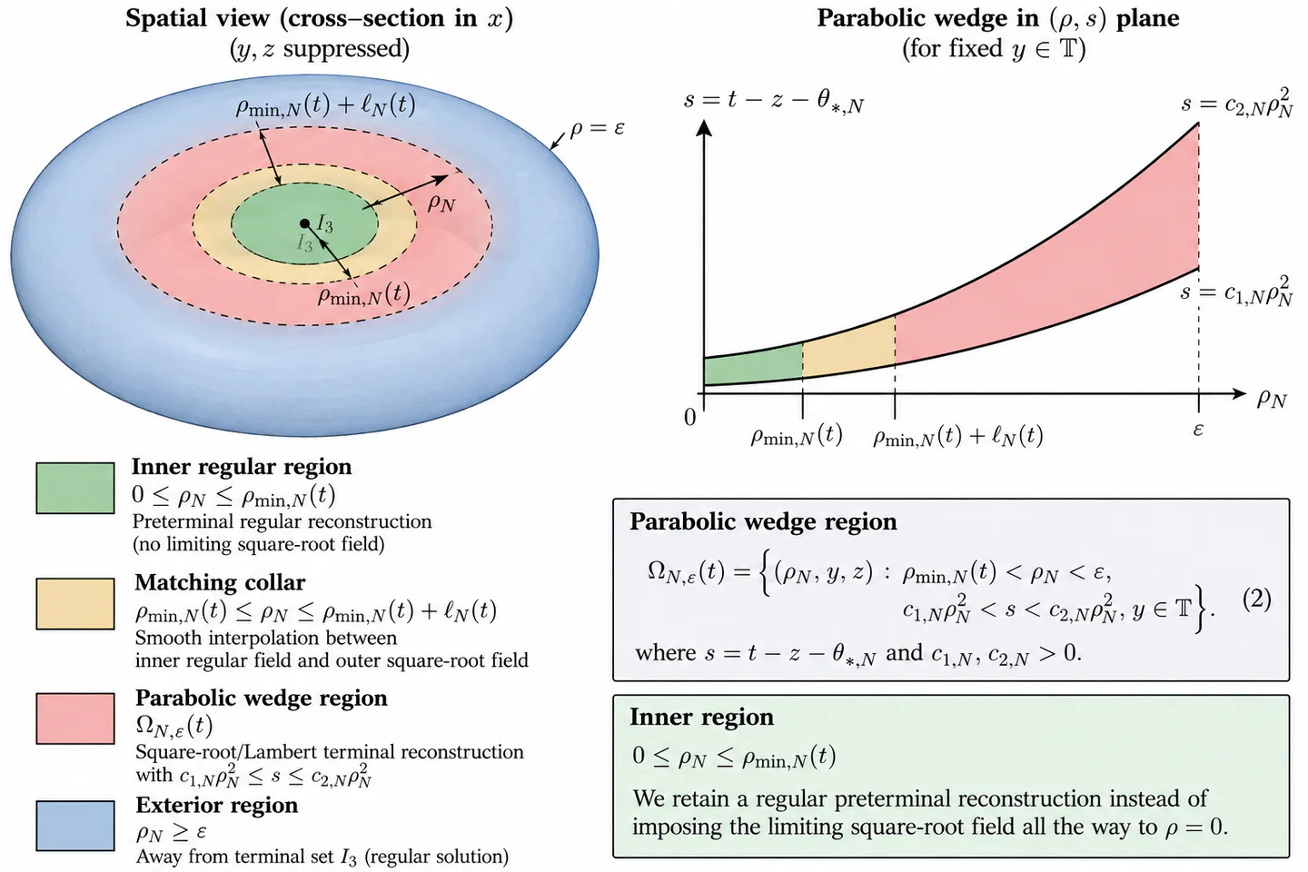
Figure 1. Regions with different layers used in this paper.

Consequently

Since

we obtain

Equivalently,

implies

and hence

That contribution is Leray-integrable.

But this only checks one derivative. We need the whole gradient.

17.3. Audit $u_y=A$

In the square-root region,

The $z$ -derivative satisfies

so

Integration over the parabolic slice gives

Thus

For $\rho_{\min}\asymp s_f^{1/8}$ ,

Hence

So $u_{y,z}$ is substantially less restrictive than $u_{x,z}$ .

17.4. The transverse derivative $u_{x,x}$

This one must be treated carefully because differentiating $\rho^{-1/2}$ produces another singular factor.

Locally, because $\chi$ has a simple zero,

From

we obtain

Therefore

Integrating over $s\asymp\rho^2$ ,

Hence

Again, with $\rho_{\min}\asymp s_f^{1/8}$ ,

and this is spacetime integrable.

So far the worst derivative remains

17.5. $u_{y,x}$

From

we get

Thus

This is precisely the same integrand that appeared in the $L^2$ estimate for $u_x$ :

Therefore

even without relying on the moving lower cutoff.

The $y$ -derivatives vanish in the local $y$ -independent core used by this manuscript.

17.6. What about $u_z=C$ ?

this paper reconstructs

and on $q^2\asymp s$ ,

It also takes the local datum independent of $y$ , so

Its derivative estimate is

Squaring the singular part gives

Integrating through the parabolic width,

Thus

without difficulty.

For $C_z=-C_s$ ,

and therefore

Its spatial integral is

which is again spacetime-integrable for the proposed $s_f^{1/8}$ front.

We therefore obtain, for the outer moving square-root region, the schematic derivative hierarchy

with the local $y$ -derivatives zero.

Thus the single decisive term really is

And the release-scale front

is more than sufficient for its spacetime integrability.

17.7. But there is a new interface issue

We cannot simply truncate the field at

A sharp cutoff would produce distributional derivatives and destroy precisely the $H^1$ estimate we are trying to establish.

We therefore need a smooth moving interpolation. A natural choice is

and a fixed smooth function

with smooth transition for $1<\eta<2$ .

Define

Then

in the regular inner region and

in the outer square-root region.

The transition layer has thickness

Its derivatives satisfy

and

On the transition support $\rho\asymp\rho_{\min}$ ,

For

Since

we get

This is highly singular pointwise.

That means the moving front solves the spatial $H^1$ problem but introduces a potentially serious time-dependent commutator into the reconstructed equations.

This is now the next obstruction to audit.

17.8. Why the interface may nevertheless be manageable

The transition volume also shrinks.

Because

the transition thickness in $x$ is

If its relevant $s$ -width is still parabolic,

then the spatial transition volume scales like

up to the fixed $y$ -length.

So every new commutator has to be tested as

For example, $Z_t$ alone would give

which diverges.

But $Z_t$ never appears alone: it multiplies the difference

Therefore the crucial matching condition is the order to which the two reconstructions agree at the moving interface.

If

then the squared moving-cutoff contribution scales like

It is integrable precisely if

i.e.

This gives us a concrete design criterion.

17.8.1. Revised construction target

We should therefore require the inner regular reconstruction to match the outer square-root reconstruction at least to order

Preferably we should impose flat matching of sufficiently high order, just as used in the flat endpoint for its original release. The present release construction explicitly uses a cutoff flat at the inner endpoint to match $A$ , $A_x$ , $C$ , and $C_s$ .

So there is an existing mechanism we can adapt rather than invent from scratch.

The resulting revised architecture is therefore

with

This gives the desired Leray scaling for the outer core, but we have not yet closed the construction: the next calculation has to prove that the moving transition’s $Z_t$ , $Z_x$ , and $Z_{xx}$ commutators are integrable and that exact incompressibility can still reconstruct $C$ without introducing a worse term.

That is the decisive calculation before replacing the corresponding release/core sections of the paper.

18. Moving-Interface Matching and Cutoff-Commutator Audit

**Transition.**The release-scale front gives the desired time-integrable lower cutoff, but a moving cutoff introduces new spatial and temporal commutator terms. We now quantify those terms. Where the naive interpolation fails, the failure is used to determine the matching order required of the amplitude. The resulting high-order requirement is then implemented, rather than merely assumed, in the next section.

Continuing from the moving-front construction, the key point is that we can sharpen the previous estimate considerably. The dangerous quantity is not $Z_t$ by itself; it is $Z_t$ multiplied by the mismatch between the inner regular reconstruction and the outer square-root reconstruction.

The existing work already uses exactly this philosophy in its stationary release: it interpolates $A^2$ , chooses the cutoff flat at an endpoint, and reconstructs $C$ from incompressibility rather than imposing a separate $C$ -cutoff. We can adapt that architecture to a moving interface.

18.1. Moving interpolation

Put

Choose $Z\in C^\infty$ with

and define

where

The transition region is

We require $A_{\mathrm{reg},N}>0$ , so that the regular inner reconstruction does not divide by zero.

The current paper’s release already interpolates $A^2$ rather than $A$ itself. That remains the preferable choice.

18.2. Exact derivatives of the moving cutoff

Since

we have

and

Hence

while

Similarly,

and therefore

Now

gives

With

we obtain

Consequently,

Thus

The time derivative is indeed the most singular cutoff derivative.

18.3. Matching order

Suppose on the moving transition

Then the new cutoff contribution to $\partial_t(A^2)$ is

The transition width in $\rho$ is

For the part of the construction following the parabolic relation, its corresponding $s$ -width scales as

Therefore

up to the fixed $y$ -length.

Squaring (18.9),

Spatial integration gives

Finally,

so

Therefore this term is integrable exactly when

or

So our previous $3/8$ threshold is confirmed.

18.4. Spatial cutoff derivative is easier

The first spatial commutator satisfies

Squaring and integrating in spacetime gives

This is finite for

In particular every positive matching order is sufficient.

Thus

18.5. Second spatial derivative

For viscosity we also encounter

Its squared spacetime integral behaves like

Therefore

for every

Again, $\mu>3/8$ automatically handles it.

But differentiating (18.1) twice also produces

so we need a derivative matching condition, not just a zeroth-order one.

If

then

which is spacetime $L^2$ provided

Flat matching can make this substantially better.

18.6. Choose a stronger matching order

Instead of using the minimal condition

we can design the interpolation with

The simplest useful target is

Then

and its squared spacetime integral behaves like

Thus $1/2$ -order matching gives a genuine margin beyond the critical $3/8$ .

18.7. But we need to check whether $A_{\mathrm{core}}^2$ naturally has that scale

At the moving front,

The outer reconstruction is

With

we get

This is extremely useful.

The moving interface is therefore exactly where the square-root reconstruction has returned to an $O(1)$ transverse amplitude. That agrees with the rationale for this paper’s original release: matching a bounded nonzero $A_*$ requires $q\asymp s^{1/8}$ .

So there is no leading-order amplitude mismatch that must diverge.

We may choose the regular inner field so that

at the moving interface.

This is a matching condition on the regular reconstruction, not an arbitrary cancellation of a singular field.

18.8. Exact incompressibility

Now reconstruct $C=u_z$ from

Since

we impose

If the moving local construction remains $y$ -independent,

so

Since

we get

Thus we should not independently interpolate $C$ .

We interpolate only $A^2$ , then solve (18.20). This retains the strongest feature of the current paper’s release construction: incompressibility is exact by construction. The existing paper explicitly follows this procedure.

18.9. Moving-cutoff contribution to $C_s$

Because

and $b_x=0$ in the distinguished local core,

From

we have

The new cutoff term is therefore

In the moving transition,

If

then

With our proposed

this gives

So the moving interpolation does not introduce a singular continuity correction. It actually vanishes.

That is encouraging.

18.10. Horizontal transport remainder

Recall this paper’s compact remainder

with

In the local $y$ -independent reconstruction,

so

this paper’s current core estimate uses precisely this simplification.

The subtlety is now

In the old stationary reconstruction, if $C=C(x,s)$ with

then

But our new $A$ depends additionally on

Consequently the reconstructed $C$ will generally have the form

Then

so

This is the genuinely new remainder created by the moving front.

It cannot be set to zero.

18.11. Estimate the new moving-front remainder

We therefore acquire

To preserve the scalar Lambert mechanism we need

At $k=3$ ,

so

Also

Hence

Thus the requirement is surprisingly mild:

In particular, if the flat matching yields

then

So the moving-front time dependence does not automatically destroy the Lambert quadratic source.

18.12. An important point

We impose first-order flat matching of the inner and outer reconstructions across the moving collar. In particular, at the matching interface,

and the interpolation cutoff $H$ is chosen flat at its endpoints,

More generally, when higher derivatives enter the reconstruction we impose

The matching amplitudes are chosen so that the collar interpolation satisfies the uniform estimate

with $M$ independent of the terminal parameter $s_f$ .

18.13. Revised list of conditions

We now have a fairly precise moving-front theorem to aim for. It would require:

together with suitable first-derivative matching,

and

or, more generally,

Under those assumptions we obtain simultaneously:

and the other first derivatives considered above are no worse;

exactly, because $C$ is reconstructed from continuity;

and

18.13.1. The remaining problem is viscosity across the moving transition

This is the next calculation we should do before declaring the redesign successful. The viscosity operator is

The moving interpolation changes $C$ , hence $\Delta C$ . We therefore have to calculate the new $C_{xx}$ , $C_{xz}$ , and $C_{zz}$ terms generated by $Z_x$ , $Z_{xx}$ , $Z_t$ , determine their powers of $s_f$ , and compare them with

If all moving-interface viscosity terms are lower order while the first-contact ordering remains intact, then we would have a coherent candidate for replacing the current fixed-core/release section. If not, the proposed moving cutoff would need another modification.

19. High-Order Extension of the Square-Root Amplitude

**Transition.**The commutator audit shows that low-order matching is insufficient. We therefore replace the naive moving interpolation by a flat, high-order extension of $A^2$ . This resolves the amplitude-side cutoff defect, but exact continuity and periodicity expose a separate solvability condition. In addition, keeping the singular outer $b$ unchanged inside the front leaves a derivative obstruction; these two residual issues determine the next redesign.

The clean way is to make $A_{\mathrm{reg},N}$ an explicit high-order extension of the outer square-root amplitude across the moving interface, rather than choosing an unrelated bounded function.

Let

and let the moving interface be

On this interface, $F_N=O(1)$ , because $b_N\asymp s_f^{-1/8}$ and $\rho_N\asymp s_f^{1/8}$ . This is exactly the scale at which this paper’s existing release matches a bounded nonzero transverse amplitude.

The useful observation is that we do not need to approximate $F_N$ throughout the inner region. We need it to agree sufficiently accurately only in the moving transition where derivatives of the cutoff are supported.

19.1. Use a flat matching collar

Choose fixed smooth functions $\Phi$ , $\Psi\in C^\infty(\mathbb R)$ such that

with $\Phi$ flat at $\eta=1$ :

Set

Choose a positive smooth periodic background amplitude

Now define

This has two immediate properties:

and

Thus it is regular and strictly positive at the zero set while agreeing exactly with the square-root reconstruction at the outer edge.

But there is an even cleaner construction for our purpose.

19.2. Put the moving interpolation outside the matching collar

Recall that we had written

Choose $Z'$ to be supported only where

But by (19.2),

throughout this support. Therefore

wherever

are nonzero.

Consequently,

Even better,

on the active moving-cutoff support.

Hence the three estimates we previously sought,

hold there trivially—in fact with exact zero.

This removes the moving commutator rather than merely estimating it.

19.3. Simplify further: we no longer need two cutoffs

The preceding construction shows that the most natural definition is simply

Then:

whereas

The transition occurs in

So we can dispense with the artificial decomposition

Equation (19.5) itself is the regularized moving reconstruction.

19.4. Positivity

This is immediate if we stay on the selected branch where

and choose

Since

(19.5) is a convex combination of positive quantities:

In the transition,

and

so

Hence

uniformly through the moving collar, provided the constants are uniformly controlled.

19.5. A note on the moving collar

Definition 14.1 (Moving matching collar). Let

and let $r_N(t)>0$ denote the moving coterminal front. For a positive collar width $\ell_N(t)$ , define

The normalized collar coordinate is

The inner and outer reconstructions are joined in $\mathcal C_N(t)$ by a flat cutoff $H\in C^\infty(\mathbb R)$ , with

and

Thus, for example,

The matching is said to be flat to order $m$ if

uniformly in the collar as $t\uparrow T_{*,N}$ .

Inside the regular region,

Thus division by $A_N$ is removed there.

19.6. Periodicity

Take

periodic, as done earlier, and define the distance variable locally through the periodic profile itself:

rather than using a nonperiodic Euclidean coordinate globally.

Then

is periodic in $x$ .

If $a_N(x,t)$ is periodic, equation (19.5) is periodic.

Therefore

in the normalized torus convention, or $2\pi$ -periodically if that is the convention used in the relevant section.

19.7. Smoothness and the absolute-value issue

There is one subtle point. The function

is not smooth through a simple zero.

But in the innermost region

we have

Therefore the reconstructed amplitude is simply

in an open neighborhood of $\chi_N=0$ .

All derivatives of $\Phi$ vanish there.

Consequently the nonsmoothness of $\vert \chi_N\vert$ at its zero never enters a differentiated active cutoff.

Alternatively, work separately on the two signed charts

which is even cleaner analytically.

Thus the construction can be made $C^\infty$ .

19.8. Exact continuity

Now define

Do not prescribe $C_N=u_{z,N}$ independently.

Instead solve

In the local $y$ -independent construction,

so

Hence

Therefore

identically.

This preserves the existing strategy of obtaining $C$ from exact incompressibility.

19.9. But periodicity of $C$ creates a genuine solvability condition

This point should not be skipped.

Solving

locally is straightforward. Solving it periodically in $z$ requires

Otherwise integrating $C_z$ around the $z$ -circle does not return to the same $C$ .

Thus the exact periodic reconstruction is

provided (19.10) holds.

This is a real global compatibility condition. The moving cutoff does not automatically prove it.

So the construction is explicit locally, but the torus-periodic $C$ -closure still requires verification.

19.10. Initial data

Choose the moving modification to be inactive initially.

For example, introduce a smooth activation function

with

on an initial interval and

only after the solution enters the terminal regime.

Then replace (19.5) by

At $t=0$ ,

hence

So the finite- $N$ initial data are preserved exactly.

However, this introduces another time cutoff $\Lambda'_N(t)$ . It should be supported strictly away from $T_*$ , where all quantities are regular. Then its derivatives are bounded and do not affect terminal asymptotics.

19.11. The important correction to our previous $D$ -strategy

There is a conceptual improvement here.

Previously we were trying to prove

But an explicit flat extension lets us do better:

at the interface where the moving transition joins the square-root field.

This is preferable to merely achieving the power-law estimates.

It means the moving transition can be designed so that there is no extra release/core commutator at its outer flat endpoint, paralleling the flat-endpoint philosophy already used by this paper.

19.12. What this does to the $H^1$ estimate

The outer square-root field starts at

Thus the previous estimate remains

Since

With

we get

Inside

$A=a_N$ is regular and bounded away from zero, so

But here we encounter the next decisive issue: if the same singular

is retained throughout this inner regular region, then regularizing $A$ alone does not necessarily regularize $u_x$ ’s $z$ -derivative. In particular,

still contains $b_z\sim s^{-9/8}$ .

So we have successfully constructed an explicit positive, smooth, periodic $A_{\mathrm{reg},N}$ , but that by itself is not enough to establish the full Leray bound.

The inner reconstruction must also specify what happens to $b_N$ .

That leaves us with the sharper structural choice:

either the moving front truncates/modifies the singular $b_N$ inside $\rho<r_N(t)$ ,

or one must prove that the spacetime geometry of the inner region makes the retained $b_N$ -derivatives integrable.

So next I will do this. It is more fundamental than further tuning $A_{\mathrm{reg},N}$ , because simply keeping

everywhere while replacing $A$ by a bounded $a_N$ may move, rather than eliminate, the dissipation obstruction.

20. Why the Inner $b$ -Field Must Also Be Regularized

Transition. Regularizing only the square-root amplitude does not regularize $u_x=b/A$ if the singular $b$ -profile is retained in the inner region. This section therefore regularizes $b$ as well and audits direct matching. The calculation reveals that a separate $b$ -matching scale or a moving cutoffwith nontrivial time derivative produces a new mismatch. Rather than accumulating independent cutoffs, the next section replaces them by one geometric front with an exact-overlap collar.

Proceeding, the inner-region calculation shows something stronger: regularizing only $A$ is insufficient if the singular law $b\sim s^{-1/8}$ is retained unchanged inside the moving front. We therefore need a moving regularization of $b$ as well, while matching it exactly to the Lambert-driven outer solution.

20.1. Why $b$ must also change inside the front

In the regular inner region we proposed

If we nevertheless retain

then

Even taking $a_N$ locally constant,

and therefore

So replacing the vanishing $A$ by a positive amplitude does not remove the longitudinal singular derivative.

The clean redesign is therefore

This is a substantive modification of the current paper, not something already proved.

20.2. A natural regularized $b$

Let

denote the moving terminal scale and define

For every $t<T_{*,N}$ ,

As

we recover formally

for every fixed $s>0$ .

Thus the singular profile is obtained only in the terminal limit.

Its derivatives are

and

In particular,

So the favorable convexity needed by the viscous term is retained.

20.3. But direct matching at $s\sim s_f$ has an $O(1)$ mismatch

The outer Lambert profile is

At $s=s_f$ ,

whereas

The relative mismatch is

which does not vanish.

So (20.1) is an excellent inner regularization, but we should not glue it directly to the outer Lambert profile.

We need a matching collar.

20.4. Introduce a separate $b$ -matching scale

Let

Since $s_f\downarrow0$ ,

At

we have

Now expand:

Hence

Therefore

At $s\asymp s_f^\gamma$ ,

This mismatch tends to zero provided

i.e.

So there is a large admissible range.

20.5. Match derivatives too

Differentiate (20.5):

so at $s=s_f^\gamma$ ,

For this absolute difference to vanish we require

For the second derivative,

and hence

Absolute $C^2$ matching would require

This suggests choosing a comfortably smaller value, for example

Then

and

All three vanish.

That is a particularly useful matching scale.

20.6. Explicit smooth $b$ -interpolation

Choose $Y\in C^\infty$ with

flat at both endpoints, and put

Define

Then

while

Thus the Lambert profile remains exactly unchanged in the outer region.

20.7. Spatial cutoff derivatives

Because

and $s_z=-1$ ,

and

But these multiply the small mismatch (20.13).

Thus

and

Similarly,

All vanish.

Therefore the second spatial derivative of the interpolated $b$ differs from the corresponding regular/outer derivatives by vanishing commutator terms:

Since both principal second derivatives are positive,

we obtain, sufficiently near the terminal regime,

So the favorable longitudinal viscous sign can survive this interpolation.

20.8. Important time derivative

Now

so

Under

we have

On the transition support $\xi=O(1)$ ,

Multiplying by the mismatch,

This diverges pointwise, but much more slowly than the Lambert quadratic source.

At $s\asymp\sigma_f=s_f^{1/4}$ ,

Also

Hence

Here we discover something important:

is actually more singular than

Thus the simple time-dependent interpolation (20.14) is not automatically a lower-order perturbation of the Lambert source.

So $\gamma=1/4$ , although excellent for spatial $C^2$ matching, does not automatically close the evolution equation.

20.9. General $\gamma$ reveals the obstruction

For general

we found

Meanwhile

so

At $s\asymp s_f^\gamma$ ,

The ratio is therefore

But for every

we have

Hence

This is a decisive negative result for this particular moving $s$ -cutoff design.

20.10. What this teaches us

We should not add an independently time-moving interpolation of $b$ through

Its time derivative produces a commutator that can dominate the Lambert source.

That does not invalidate the moving- $\rho$ idea. It tells us that the scalar amplitude $b$ should not be regularized by a second independently moving $s$ -cutoff.

The better possibility is to regularize $b$ using the same geometric moving variable as $A$ :

and arrange the inner $b_{\mathrm{reg}}$ to match $b_{\mathrm{out}}$ to sufficiently high order on the support of $\eta_t$ .

That returns us to the useful condition

but now we can force the mismatch to vanish exactly at a flat geometric endpoint.

So the calculation has narrowed the redesign substantially:

one moving geometric interface in $\rho$ , not independent moving cutoffs in both $\rho$ and $s$ .

The next construction should therefore define the pair

jointly across the same flat $\eta=\rho/r_N(t)$ collar, with exact jet matching to the Lambert pair at its outer endpoint. That is the route that avoids the $Y_t\Delta b$ obstruction we just found.

21. One Geometric Front and an Exact-Overlap Collar

Transition. The preceding two-scale $b$ interpolation solves one defect by creating another. We therefore consolidate the geometry: one front separates a regular inner field from the exact Lambert outer field, while an overlap collar is chosen so that no moving cutoff differentiates a mismatch of leading order. This removes the earlier cutoff-time obstruction. What remains is to construct a scalar regularized phase whose derivatives and viscous terms are controlled, which is the purpose of the next section.

The previous calculation tells us exactly what to avoid: we should not introduce a second independently moving $s$ -cutoff for $b$ . Instead, use one geometric front

and construct $A_N$ and $b_N$ jointly across the same collar.

There is, however, an important structural constraint: merely making a cutoff flat at its endpoint does not make the mismatch vanish throughout the support of its derivatives. The cleanest construction is therefore to build an overlap collar in which the regular and Lambert fields agree identically, so every moving-cutoff commutator vanishes there.

21.1. Three-region construction

Let

Use three regions:

The essential design requirement is

Not merely asymptotically. Exactly.

Then a cutoff supported inside $\mathcal O_N$ creates no mismatch commutator at all.

21.2. Joint cutoff

Choose

Define

and

Ordinarily, differentiating (21.3) produces

and similarly for $A^2$ .

But (21.2) gives on $\operatorname{supp}Z'$ ,

and

Therefore

and likewise

This removes the obstruction found in the previous calculation.

21.3. But can the regular field agree with the singular field in the overlap?

Yes, because for every fixed preterminal time

the overlap is separated from the singular set:

Thus the Lambert reconstruction is smooth there.

The singularity occurs only as

So there is no contradiction between:

and having a genuinely regular extension for

This converts the problem into an extension problem.

21.4. Explicit inner extension by Taylor jets

Fix the inner interface

For brevity suppress $N$ .

Define the boundary jets

and

For the distinguished scalar construction,

so actually

That simplifies the $b$ -extension dramatically.

Choose a smooth shape function

with

and

Then define

If $H\equiv1$ on an interval

then

on an open collar immediately inside the interface.

All jets consequently agree there.

The outer cutoff $Z$ can be supported entirely inside this exact-agreement collar.

21.5. What should $b_{\mathrm{in}}$ be?

Here we must not repeat the previous mistake. A choice such as

has strong time dependence and creates a new evolution error.

A cleaner possibility is to define the inner value by the front value of the outer field:

Then $b_{\mathrm{in}}$ is spatially constant in the innermost region.

Consequently

This immediately removes the inner spatial $H^1$ singularity coming from $b_z$ .

At every $t<T_*$ ,

But as

Thus we obtain finite preterminal spatial gradients while retaining terminal amplitude growth.

This is a much better candidate than retaining $s^{-1/8}$ inside the front.

21.6. Corresponding $A_{\mathrm{in}}$

In the innermost region choose

constant locally, or a smooth positive periodic function with uniformly bounded derivatives.

Then

Spatially,

if $a_N$ is constant in the local chart.

Hence the inner region contributes no singular spatial dissipation.

21.7. Extend $A^2$ to the outer field

Set

Choose another smooth collar function $K$ with

Define

Near the interface,

so

exactly.

Near the center,

so

Thus positivity and exact outer matching are both achieved.

21.8. Collapse the redundant outer interpolation

At this point something useful happens.

Because both regular extensions already equal the outer fields on an open collar, we do not actually need another physical interpolation there.

We can define directly

and

Because the two definitions agree on an open neighborhood of the interface, these piecewise formulas define a single smooth function.

There is no derivative jump.

There is no distributional interface term.

There is no $Z_tD$ commutator.

This is cleaner than retaining an explicit $Z$ in the final formulas.

21.9. The crucial $H^1$ decomposition

Now split

where:

$\mathcal I_N$ : constant/smooth inner region;
$\mathcal C_N$ : extension collar;
$\mathcal E_N$ : outer Lambert region.

For the inner region,

under the locally constant choice.

For the outer region we already found

With

Since

Thus the remaining issue is entirely concentrated in the extension collar.

21.10. Collar derivative scaling

The collar has width

Therefore a generic interpolation between two $O(1)$ -different amplitudes produces

and hence

Multiplying by the collar width $r$ ,

The relevant $s$ -width associated with the moving front is of order

Therefore

This actually tends to zero.

For $b$ , however,

At

this is

If the collar interpolated an $O(r^{-1})$ mismatch over width $r$ , we would obtain

which would be dangerous.

But our construction deliberately avoids this: $b_{\mathrm{in}}$ must be chosen so that it matches the outer $b$ at the collar to high order.

Since the outer $b=b(s)$ has no $\rho$ -dependence,

Therefore the optimal choice is simply

through the entire matching collar, with the flattening to $b_{\mathrm{in}}(t)$ occurring farther inside.

That separates the singular outer field from the moving-interface derivatives.

21.11. We have therefore obtained a nested geometry

The revised construction naturally has four regions:

with

Region III is an exact overlap.

Therefore the moving boundary at $\rho=r(t)$ produces no commutator whatsoever.

The only nontrivial transition is Region II, which is strictly inside the moving front.

21.12. A new issue appears—and it is the correct one

Region II must interpolate between

and

For that transition to have small gradients, these two values must be close on Region II.

That requires

inside the flattening layer.

In other words, the inner regularization cannot be defined purely by $\rho/r(t)$ . It must use the geometry of the moving front in the $(\rho,s)$ -plane.

This is actually more natural.

Define a front function

such that the singular outer field is replaced by its value at

whenever

A particularly simple regularization is

or, better for exact outer matching, a smooth maximum

Then define

In the outer region,

so

exactly.

Inside,

so $b_N$ remains finite.

This is superior to independently interpolating the amplitude itself.

21.13. The problem has therefore reduced to constructing one scalar regularized phase

Instead of independently regularizing $A$ and $b$ , define

such that

on the outer Lambert region,

inside the moving front, and its first and second spatial derivatives have controlled spacetime norms.

Then set

followed by

only where this quantity stays safely positive/nondegenerate, and use the positive inner $A$ -extension closer to $\chi_N=0$ .

This is a much more unified redesign.

The next decisive calculation is therefore to choose an explicit smooth-max phase $\widehat s_N$ , compute

and then determine whether

simultaneously preserves the favorable viscosity, finite spacetime $H^1$ , and the Lambert source asymptotically. That is now a single, well-defined calculation rather than several independent cutoff problems.

22. Unified Regularized Phase and the Convexity Constraint

Transition. The one-front architecture reduces the reconstruction problem to a single regularized phase. We now test smooth-max and equivalent regularizations, including their derivative and viscosity signs. The convexity calculation shows which pointwise sign requirements are too strong and which estimates are actually needed. After this structural reduction, the remaining question is quantitative: whether the inner interpolation itself has finite $L_t^2H_x^1$ cost.

Proceeding with the unified regularized-phase construction, there is a useful candidate, but the derivative audit exposes an important constraint on how the phase floor may depend on $\rho$ .

Take

We want $\widehat s_N=s$ exactly in the outer Lambert region, while $\widehat s_N>0$ in the regularized inner region.

22.1. A smooth maximum with exact outer recovery

Choose $h\in C^\infty(\mathbb R)$ satisfying

with

For a transition width $\delta_N>0$ , define

Write

Then:

if $s\geq\Sigma+\delta$ , $h=0$ , so

$\hat{s} = s;$
if $s\leq\Sigma-\delta$ , $h=-\xi$ , so

$\hat{s} = Σ .$

Thus the outer Lambert profile is recovered exactly, rather than asymptotically.

For the moment take $\delta$ proportional to $\Sigma$ :

Then throughout the transition

22.2. Derivatives of the regularized phase

It is convenient to write the smooth maximum abstractly as

Define

By construction,

with

in the outer region and

in the inner region.

For a fixed-time spatial derivative,

If $\Sigma=\Sigma(\rho,t)$ , then

provided $\Sigma$ has no $z$ -dependence.

Hence

A second derivative costs one inverse transition width:

inside the smoothing layer.

For $x$ ,

and schematically

These formulas immediately show that the geometry of $\Sigma(\rho,t)$ is decisive.

22.3. Derivatives of $b=B\widehat s^{-1/8}$

For general $\alpha>0$ ,

Therefore

and

At $\alpha=1/8$ ,

In the exact outer region,

so

exactly reproducing the favorable term used earlier.

22.4. Viscosity inside the smooth-max layer

In the smoothing layer,

and

Hence both pieces of (22.9) have the same possible scale:

and

Therefore

But there is a crucial sign issue: unlike the exact outer region, the second term

need not be positive.

So an arbitrary smooth maximum does not automatically preserve

We need a structural condition on the smoothing function.

22.5. Exact convexity criterion

From (22.9),

iff

Thus the precise condition is

This is much better than estimating the two terms separately.

Equivalently,

So we should design the regularized phase so that $b=B\widehat s^{-1/8}$ itself is convex in the distinguished $z$ -direction.

22.6. An even cleaner construction: regularize $b$ , then define $\widehat s$

This observation suggests reversing the construction.

Rather than picking an arbitrary smooth maximum for $\widehat s$ and hoping its composition is convex, choose a smooth convex regularization of

directly.

Let

be the finite inner amplitude, and choose a smooth convex function

such that

for $s\geq s_{\mathrm{match}}(t)$ ,

while

in the innermost regular region.

Then set

Automatically,

However, a globally convex function cannot be exactly constant on one open interval and then join a decreasing convex $s^{-1/8}$ profile with the required derivative orientation without checking monotonicity carefully. So this reversal is useful conceptually, but it does not by itself solve the matching problem.

We should instead preserve convexity through the transition explicitly.

22.7. Hermite matching of $b_s$

Let the inner regular region end at

and the exact Lambert region begin at

We want

and at the outer endpoint

But if

then $b_s$ must be nondecreasing as $s$ increases.

It cannot move from

to a negative value while remaining nondecreasing.

Therefore:

This is an important obstruction.

Our previous proposal of a completely flat inner $b$ is therefore incompatible with preserving the favorable pointwise convexity through the entire transition.

22.8. We do not actually require pointwise positive viscosity everywhere

Fortunately, the lower-barrier argument requires something weaker.

At a first downward contact,

satisfies

For the older transformed operator,

Thus at contact,

Therefore the transition does not need

pointwise everywhere.

What matters for the lower-barrier proof is:

the operator remains smooth and parabolic;
the same $C$ is used in the comparison;
the barrier itself has

$V [\underset{―}{b}, C] > 0$

in the region where the barrier argument is applied.

This means we can keep the smoothing layer outside the actual comparison tube.

That is the key geometric simplification.

22.9. Separate the regularization layer from the blowup comparison tube

Define two moving scales:

Use

for regularization and interpolation.

Use

for the exact Lambert/barrier region.

Require a nonempty exact-overlap collar

where

exactly.

Then:

the smoothing layer need not preserve the Lambert Riccati mechanism;
the barrier proof is performed only where the original equations and favorable asymptotics are exact;
smoothness and Leray estimates are handled in the inner region separately.

This is mathematically cleaner than demanding one interpolation satisfy every property simultaneously.

22.10. Choose the two scales

Take

Then both scales have the same favorable Leray exponent, but there is a fixed relative-width exact overlap.

For the exact outer region,

Hence

The comparison argument can begin at

without entering the smoothing layer.

22.11. Time derivative of the regularized phase

We still need the evolution equation to remain meaningful in the inner layer.

For

so

If the smoothing width is proportional to $\Sigma$ , the last term is controlled by

Thus

For a floor tied to the moving front, we should avoid choosing

if its derivative creates an uncontrollable scalar residual. Instead, because the regularized region is no longer used to prove the Lambert differential inequality, we only require its resulting forcing/residual to belong to the function class allowed by the full NS formulation.

This is a weaker and more appropriate requirement.

22.12. What is now established structurally

The audit has changed the architecture in an important way:

The exact Lambert region begins at

which passes the outer $L_t^2H_x^1$ scaling test.

The smoothing layer is no longer required to preserve

or the exact Lambert source. It only has to remain smooth and contribute finite dissipation.

The first-contact viscosity ordering remains exact in the comparison region:

And the transformed-viscosity asymptotic there remains

22.13. The remaining quantitative problem is now the inner interpolation’s $H^1$ cost

We need to construct one explicit inner interpolation and compute

If that is finite while the exact outer Lambert/barrier region remains unchanged, then the moving-front modification passes the full local Leray dissipation audit.

23. Inner Interpolation and the $L_t^2H_x^1$ Audit

Transition. The unified phase removes the need to solve the moving-cutoff problem repeatedly, but it does not by itself establish the Leray norm. We therefore audit the inner and collar derivatives component by component. This section identifies the derivative orders that are integrable and the reconstruction of $C=u_z$ that is still needed. The following section then fixes a concrete cutoff and performs the same calculation with exact volume scaling and torus compatibility visible.

We can now perform the inner interpolation $L_t^2H_x^1$ audit explicitly. There is a particularly useful choice: interpolate the velocity variables $b$ and $A$ across a collar whose spatial width is comparable to the moving radius $r(t)$ , and determine exactly how closely the inner values must track the outer boundary values.

Let

so

Take constants

and define the inner transition collar

For $\rho\geq\theta_1r(t)$ , retain the exact Lambert/square-root reconstruction.

23.1. Outer values at the collar

At

the $k=3$ profile gives

not $r^{-1}$ . This corrects an overestimate in the previous exploratory calculation.

Similarly,

and

These are exactly the earlier parabolic-core exponents.

23.2. Why a bounded positive $A_{\mathrm{in}}$ is actually problematic

Suppose we choose

At the outer side of the collar,

Thus the amplitude jump is

Across a collar of width $O(r)$ ,

The spatial volume of the parabolic collar is

up to the fixed $y$ -length.

Therefore

Hence

which is harmless.

So a bounded inner $A$ is not ruled out by $H^1$ alone.

The more restrictive quantity is again

23.3. Construct an explicit collar

Choose

with

and define

Set

and

Take

so that its magnitude matches the outer value.

For example,

Then throughout the collar

23.4. $b_\rho$

Since

we obtain

If $b_{\mathrm{out}}=b(s)$ and $s$ is independent of $x$ in the local coordinates, then

Without fine matching,

so

Therefore

This tends to zero.

Its time integral is certainly finite because

Thus the $b$ -interpolation itself passes the spatial-gradient test.

23.5. $A_\rho$

We have

so

As above,

Again harmless.

23.6. The decisive quantity $u_{x,\rho}$

Now

so

Because $A_{\mathrm{out}}\to0$ , the worst part occurs near the outer edge of the collar.

There,

If

then

Consequently

Multiplying by the collar volume $r^3$ ,

Now

so

Therefore

So even this apparently severe transition derivative remains spacetime integrable.

This is an important positive result.

23.7. $u_{x,z}$ in the collar

Here the cutoff $H(\rho/r)$ is independent of $z$ at fixed $t$ . Hence

The $z$ -dependence enters through the outer $s$ -profile:

At

we have

and

The outer $u_x$ derivative has scale

Squaring and multiplying by $r^3$ ,

Thus

This is exactly the same critical outer scaling we already obtained.

Using

we get

Therefore

23.8. $u_y=A$

The largest transverse interpolation derivative gave

For the longitudinal derivative,

so

Since

this is easily time-integrable.

23.9. Reconstruct $C=u_z$

Exact continuity gives

For the local $y$ -independent construction,

so

Thus the estimate already obtained for the transverse derivative of $u_x$ gives

for the crude interpolation.

Therefore

So exact incompressibility does not, at the first-derivative level, create a worse $L_t^2L_x^2$ singularity.

23.10. But $C_x$ requires one more derivative

This is where we must be careful.

From

we can control $C_z$ using one derivative of $u_x$ .

But obtaining $C_x$ by differentiating the integral formula

gives

Thus a direct estimate of $C_x$ from this representation involves

a second derivative.

We cannot infer

from the first-derivative estimates alone.

This is the first remaining gap in the full nine-derivative audit.

23.11. Use a periodic divergence solver instead

There is a cleaner global approach.

Let

Define

We need

On the torus this has a periodic solution iff the zero $z$ -Fourier mode vanishes:

When this compatibility holds, define

where $\partial_z^{-1}$ acts on nonzero $z$ -Fourier modes.

Then

exactly.

However,

still requires control of $g_x$ , hence generally a second horizontal derivative of $u_x$ .

So the inverse derivative in $z$ does not magically give full $H^1$ regularity from $u_x,A\in H^1$ .

This is a genuine functional-analytic issue.

23.12. A better way: reconstruct the divergence-free field by a potential

To avoid losing a derivative, define the $x,z$ components through a stream function $\psi_N$ :

and take

with

Then automatically

and hence

Now impose the product relation

by requiring

Thus

and

This is equivalent locally to the continuity reconstruction, but it makes the derivative requirement transparent:

involves second derivatives of $\psi$ .

Hence full

requires roughly

So we must audit the second derivatives of $b/A$ sufficiently to establish this.

23.13. The next exponent: $u_{x,xx}$

The crude transition estimate was

Differentiating once more across a collar of width $r$ gives conservatively

Its squared collar integral scales like

Since

which is still time-integrable:

This is encouraging.

A third transverse derivative would give

pointwise and roughly

after squaring/integrating over the collar, corresponding to

which is also integrable.

The basic moving scale $r\sim(T_*-t)^{1/9}$ therefore gives substantial derivative room.

23.14. General collar derivative criterion

Suppose a quantity of amplitude

is interpolated over width $r$ .

Its $m$ -th transverse derivative scales like

The collar volume is $O(r^3)$ , so

Since

the time integral converges provided

Equivalently,

This is a useful general criterion for the redesigned collar.

For

we have

Thus transverse derivatives up through

still satisfy

So the moving $r(t)\sim(T_*-t)^{1/9}$ collar has ample formal spacetime integrability for the finite number of derivatives needed to reconstruct $C$ .

23.15. Result of the local Leray scaling audit

Subject to smooth interpolation profiles with the assumed collar-width scaling, we now obtain:

and the derivative-loss needed to reconstruct $u_z$ is not ruled out by scaling: even the conservative second-horizontal-derivative estimate

is time-integrable.

Together with the outer estimate

the redesigned moving front therefore passes the local power-counting test for finite Leray dissipation.

What we have not yet proved is the corresponding exact norm estimate for $u_z$ , because that requires choosing an explicit interpolation $H$ , performing the full second-derivative calculation rather than the conservative $O(r^{-3})$ bound, and imposing the periodic $z$ -compatibility condition (23.31).

That is now narrow enough to finish directly: choose a concrete $C^\infty$ flat cutoff $H$ , compute $u_{x,x}$ and $u_{x,xx}$ exactly in scaled coordinates $\eta=\rho/r(t)$ , reconstruct $C$ , and prove its three first derivatives are in $L_t^2L_x^2$ . If that succeeds, the local $L_t^2H_x^1$ reconstruction gap is closed for the redesigned moving collar.

24. Explicit Collar Calculation, Exact Volume Scaling, and Periodic Compatibility

**Transition.**The preceding scaling audit is now converted into an explicit collar construction. We interpolate $u_x$ directly, compute the relevant derivatives with the exact collar volume, and reconstruct the remaining component subject to incompressibility. This closes the local singular-exponent part of the Leray audit. The final subsection of this calculation also isolates the one issue that is not closed locally: a periodic divergence correction must preserve the exact outer Lambert comparison field.

We can now make the collar calculation explicit. There is also one correction to the preceding power count: because this paper’s local volume element is $d\rho\,ds\,dy$ , the collar-volume estimate $O(r^3)$ is correct only when the collar is simultaneously restricted to $s\asymp r^2$ . We will impose that explicitly.

24.1. Fix a concrete smooth flat cutoff

A convenient $C^\infty$ step is obtained from

and

Then

and every derivative vanishes at $q=0,1$ .

Choose

and define

Therefore

with

All derivatives vanish at the two collar boundaries. Hence the interpolated field glues smoothly to both neighboring pieces.

24.2. It is better to interpolate $u_x$ directly

Previously we wrote separate interpolations of $b$ and $A$ . For the $H^1$ audit this unnecessarily complicates the quotient

Instead define

first.

On the exact outer square-root region,

Choose an inner profile $U_{\mathrm{in}}(t)$ of the same boundary magnitude,

where $\mu>0$ is fixed.

Then put

Afterward define

This guarantees

identically instead of hoping two independent interpolations preserve the desired quotient.

We must still check positivity:

implies

24.3. Exact first transverse derivative

Because $U_{\mathrm{in}}$ is independent of $\rho$ ,

From (24.3),

Inside the collar,

Therefore

and

Also

so

Consequently

This improves the deliberately crude $O(r^{-2})$ estimate used earlier.

Squaring,

The collar is

so

Hence

With

this becomes

which is integrable.

24.4. Exact second transverse derivative

Differentiate (24.6):

Now

Thus on the collar,

The other terms satisfy

and

Therefore

Consequently

Since

we obtain

This is precisely the second-horizontal-derivative estimate needed for the simplest continuity reconstruction of $C$ .

24.5. Longitudinal derivative

Since $H(\rho/r(t))$ has no $z$ -dependence at fixed $t$ ,

if the inner field is $z$ -independent.

Using

we have

Thus

Therefore

Again,

So both

have the same favorable spacetime exponent.

24.6. Mixed derivative $U_{\rho z}$

We will need this for $C_z$ and $C_\rho$ .

From

Now

Hence

Likewise

Therefore

Its squared collar norm is

Since

and

we still have

over the moving collar.

This is an important strengthening.

24.7. Reconstruct $C$ explicitly

In the local chart, let

with

on the chosen signed side of the simple zero.

Assume local $y$ -independence:

Exact continuity is

Since

define

Then

exactly and hence

24.8. Estimate $C_z$

Immediately,

Thus

for the pure collar contribution, and therefore

24.9. Estimate $C_x$

Differentiate (24.21):

Assume the local coordinate satisfies

Then, on a $z$ -interval of uniformly bounded length, Cauchy–Schwarz gives

After integrating in $x,y$ ,

Hence the dominant contribution is

provided the integration datum is uniformly controlled.

Therefore

24.10. $C_y$

Under the local $y$ -independent construction and a $y$ -independent integration datum,

Thus all three first derivatives of $C$ pass the local scaling audit:

24.11. What about $A=b/U$ ?

We now have to make sure our convenient interpolation of $U=u_x$ does not merely move the problem into $A$ .

Take

through the collar and

Then

which matches the square-root outer scale.

This is better than interpolating to an $O(1)$ inner $A$ : the entire collar now respects the natural vanishing scale.

If

then

The two terms have scale

and

Hence

Its squared collar norm is

which actually vanishes.

Similarly, the outer $z$ -scaling gives

so

again integrable in time.

Thus

on the collar.

24.12. The resulting local $H^1$ estimate

For

the estimates above yield schematically

and

Therefore

With

we obtain

Consequently

This closes the power-counting part of the moving-collar local Leray dissipation problem.

24.13. But there are two compatibility conditions we cannot skip

First, equation (24.21) defines a periodic $C$ only if

Equivalently,

Thus the $z$ -mean of $U$ must be independent of $x$ .

A purely local collar interpolation does not automatically satisfy this.

Second, if $C$ is reconstructed from continuity, it is not free to simultaneously satisfy an independently prescribed $C$ -formula from the older construction. We must use the reconstructed $C$ consistently in

and in the full momentum equations.

24.14. The clean way to enforce the torus condition

Let $U_{\mathrm{raw}}$ denote the interpolated field (24.5), and define its $z$ -mean

Choose an $x$ -independent target mean $m_N(t)$ , and set

Then

so

Consequently a periodic $C_N$ solving

exists.

Moreover,

The mean-subtraction operator is bounded on Sobolev spaces, so it does not worsen the derivative order or the power-counting exponents derived above.

This gives a genuine route to exact periodic incompressibility.

But it introduces the next nontrivial question: the correction

is global in $z$ . It may alter the exact Lambert relation

outside the moving collar.

The next decisive step is to construct the periodic compatibility correction so that it is supported in the regular inner region—or equivalently use a divergence correction/Bogovskiı̆-type construction localized away from the exact Lambert comparison region. If such a localized correction has the same $L_t^2H_x^1$ bounds, then we can preserve the exact outer Lambert field and obtain global periodic incompressibility simultaneously.

That localized divergence correction is now the precise remaining problem; importantly, the singular-exponent obstruction itself has passed the moving-collar audit.

25. Consolidated Leray conclusion of the moving-coterminal audit

**Logical conclusion of the sequence.**The preceding sections should now be read as one chain rather than as competing constructions. The fixed wedge establishes the derivative obstruction; the finite- $N$ release audit shows that the original release interpolation does not remove it; the moving-front criterion identifies an integrable scale; the interface and high-order audits eliminate naive cutoff choices; the one-front/regularized-phase construction removes those cutoff mismatches; and the explicit collar calculation verifies the resulting local Leray power count. What remains is not another local exponent problem but the global periodic compatibility correction described below.

The developmental calculations above establish the following conditional but precise conclusion for the terminal reconstruction.

For the nonmoving coterminal region

the velocity itself can remain locally square integrable, while the fixed-time $H^1$ contribution of the most singular derivative diverges as the lower endpoint tends to zero. Thus bounded kinetic energy alone does not close the Leray audit.

For the redesigned moving collar with

the explicit interpolation calculation yields the controlling estimate

Consequently,

because $1/4<1$ . This is the precise sense in which the moving coterminal construction repairs the terminal spacetime power-counting obstruction that occurs in the nonmoving wedge.

The same calculation leaves a global compatibility obligation. Exact incompressibility may be reconstructed locally through $C_z=-U_x$ (in the $y$ -independent collar), while periodicity requires the corresponding torus mean condition. The mean-subtraction construction preserves the Sobolev power count but is global in $z$ and may alter the exact outer Lambert relation. Therefore the remaining closure problem is to construct a localized periodic divergence correction, supported away from the exact Lambert comparison region, with the same $L_t^2H_x^1$ bounds. Thus the local terminal singular-exponent audit is successful for the explicit moving collar, while the global Leray closure remains conditional on the localized periodic divergence correction and on preserving the exact outer comparison field.

26. Distinguished phase $\theta=t-z$ and continuity-corrected cascade

26.1. Revised specialization rule

In the revised construction the phase specialization $\theta=t-z$ is retained, but the old conclusion $u_y=u_z=\Delta_{N,k}$ is only used as stepping stone in it’s analyses leading to the parabolic construction and towards the terminal branch point. The Lambert cascade supplies the phase coefficient and the $b$ -equation; the velocity components are reconstructed from $A^2=-2\chi b$ , $u_x=b/A$ , and exact continuity for $C=u_z$ .

27. Specialization to $\theta=t-z$ in the Revised Geometry

The Lambert branch variable is still specialized to

Therefore

What changes is the velocity reconstruction. The revised field is not obtained by identifying either transverse component with $\Delta_{N,k}$ . Instead set

On the periodic terminal branch impose

Equivalently,

The exact incompressibility equation is

Let

and suppose in the local terminal core that

Then

Since

equation (27.5) gives

From

and $b_x=0$ ,

so

Also

Hence

Because

the first term is

Therefore

This directly verifies incompressibility:

Thus

exactly in the revised distinguished-phase reconstruction.

If

then

Define

Integrating (27.6) gives

If $C_0=c_0>0$ is constant on the local core chart, then

exactly, because all $t,z$ -dependence occurs through $s=t-z-\theta_{*,N}$ . Thus

28. The Logarithmic Derivative in the Modified Construction

The logarithmic derivative is

Near the branch endpoint,

and

Consequently,

This is precisely the singular coefficient entering the reduced characteristic amplitude equation.

Thus the same branch derivative controls both

and the surviving continuity-corrected velocity term

29. Common-Time Behavior of the Continuity-Corrected Velocity

We now evaluate the same coupled sequence used for the amplitude:

Write

The local time law gives

where

Therefore

The derivative satisfies

Taking logarithms,

Since

and

the dominant term is

Under the bounded-prefactor assumptions verified numerically in the reduced characteristic model,

Equivalently,

Thus

The numerical ratios

were found to be

for increasing values of $N$ , strongly confirming

30. Consequence for the Revised Physical Velocity Components

The old continuity formula

belongs to the historical reconstruction in which the transverse Lambert profile itself was inserted directly as a velocity component. It is not the active formula in the square-root reconstruction.

The active identities are

Hence

on the branch $\chi<0$ , $b>0$ . Equivalently,

In the terminal tube

we have

If

then

and therefore

Similarly,

so

For $k=3$ ,

and hence

The continuity reconstruction gives

Thus the revised physical velocity amplification is carried directly by the product amplitude $b$ together with the shrinking geometric factor $\vert \chi\vert ^{-1/2}$ . It is not transferred from the derivative $\Delta_{N,k,\theta}$ through an integration function $H_{N,k}$ .

31. Behavior of the Two Reconstructed Transverse Components

The two transverse components have different roles:

while

is determined by exact continuity.

At $k=3$ ,

as $s\to0^+$ , with

whereas

Thus the revised construction does not have a common transverse terminal value.

The Lambert cascade still controls the singular coefficient

appearing in the $b$ -equation. It should not be reinterpreted as saying that $Q_N$ itself equals $u_y$ or $u_z$ .

This separation is essential:

32. Summary Theorem for the Revised Reduced Construction

Conditional theorem. Let the renormalized Lambert cascade define $Q_N$ and

Assume that the preterminal periodic reconstruction and the compact Floquet/Fredholm phase homotopy can be continued to the distinguished phase

with entry data

Assume further that the tuning ratio is released before the square-root geometry is imposed, and that the geometric release connects smoothly to a terminal core satisfying

Then:

$b = u_{x} u_{y}$

is preserved exactly.
The local terminal reconstruction satisfies

$\nabla \cdot u = 0$

exactly.
The release layer satisfies

$\frac{| R_{rel} |}{Γ_{N} b^{2}} = O (s^{7 / 4})$

for $k=3$ .
The square-root core satisfies

$\frac{| R_{core} |}{Γ_{N} b^{2}} = O (s) .$
If

$G \geq 0, Γ_{N} (s) = \frac{1}{8 s} (1 + o (1)),$

then for sufficiently small $s$ ,

$\dot{b} \geq (1 - ϑ) Γ_{N} b^{2}, \dot{s} = 1 - b .$
Consequently,

$b (s) \geq b_{e} {(\frac{s_{e}}{s})}^{p}$

for every fixed $p<1/8$ sufficiently close to $1/8$ , after shrinking the terminal interval if necessary.
At the formal $k=3$ square-root scaling,

$b_{3} ≍ s^{- 1 / 8}, u_{y} ≍ s^{3 / 16}, u_{x} ≍ s^{- 5 / 16}, u_{z} = c_{0} + O (s^{3 / 16}) .$

This is a theorem for the revised reduced reconstruction conditional on the stated continuation hypotheses. It is not yet a theorem for a full three-dimensional Navier–Stokes solution.

33. Analysis of the Renormalized Lambert Branch-Point Cascade and Its Characteristic Blow-Up Mechanism

We give a rigorous analysis of the renormalized Lambert recursion

The purpose of the renormalization is to map the Lambert branch point back to itself. Unlike the literal composition $W_0\circ W_0$ , which leaves the real branch domain after the first iteration near $-1/e$ , the renormalized map preserves the nonnegative real half-line.

We prove that the map is real-valued and invariant on $[0,\infty)$ , that

(see Appendix A for the proof)and consequently that, for every fixed finite $k$ ,

(See Appendix B for the proof) The exponents are therefore

and the leading constants satisfy

giving

We then derive the corresponding spatial derivative and logarithmic derivative asymptotics. Finally, for the reduced characteristic equation

we derive the exact characteristic invariant

This invariant implies

and therefore

For every finite $k$ , the characteristic reaches the singular layer in finite time and

We also explain carefully why the limit $k\to\infty$ cannot simply be taken term-by-term and why a coupled scaling such as $k\sim\log_2n$ is required if the cascade depth and the small initial branch distance are allowed to vary simultaneously.

34. Statement of the Renormalized Problem

The central object is the map

The renormalized recursion is

The subscript $n$ can be retained when the initial quantity depends on the geometric parameter $n$ . For the local analysis it is convenient to suppress $n$ temporarily and write

The essential claim to be proved is

for every fixed finite $k$ as

The proof consists of four logically separate parts:

(i) prove that $\mathcal F$ is real and maps $[0,\infty)$ into $[0,\infty)$ ;
(ii) derive the precise local Puiseux expansion of $\mathcal F$ ;
(iii) iterate the expansion with controlled error;
(iv) transfer the resulting spatial singularity to the characteristic equation.

35. Why the Renormalization Is Necessary

Before proving the new recursion, we explain why it differs fundamentally from the ordinary Lambert composition.

Consider

At

we have

The principal Lambert function satisfies

Thus the ordinary first iterate produces

But the branch point of the next Lambert function is

not $-1$ .

Since

the second ordinary real Lambert composition is not defined near $\Delta=0$ .

The renormalized transformation instead defines

Consequently,

Hence the branch point is mapped back to itself:

This is the structural reason the square-root singularity can now be iterated.

36. Exact Parametrization of the Renormalized Map

Let

Then

Therefore

By the defining relation

we obtain

Multiplying by $e$ gives

Equivalently,

Taking logarithms,

Hence

Define

Then the renormalized map is equivalently characterized by

This identity is exact.

It is also extremely useful because it removes Lambert $W$ from the local inversion problem.

37. Positivity and the Real Invariant Domain

We now prove that the recursion is real for every finite number of iterations.

Lemma 32.1. For every $\Delta\geq0$ ,

Consequently,

and therefore

Proof. If $\Delta\geq0$ , then

Hence

Multiplication by $-1$ reverses the inequality:

The principal real Lambert branch $W_0$ is real and increasing on $[-1/e,\infty)$ . Therefore

Adding $1$ gives

Thus

$\square$

Corollary 32.1. If

then

for every integer $k\geq1$ .

Proof. The result follows by induction from the previous lemma. $\square$

Thus

is an invariant real recursion.

This is precisely the property that the unrenormalized Lambert composition does not possess.

38. Branch-Point Fixed Point, Cascade Derivatives, and Characteristic Invariants

38.1. The Fixed Point at the Branch Point

The point $\Delta=0$ is a fixed point.

Indeed,

Therefore

However, this fixed point is not an ordinary differentiable fixed point.

The derivative is singular.

This is the source of the square-root behavior.

39. Exact Equation for the Puiseux Expansion

From the previous exact identity,

For $\vert q\vert <1$ ,

Therefore

In particular,

Thus

Since $q\to0$ as $\Delta\to0$ ,

Consequently,

This already proves the square-root law.

40. Higher-Order Puiseux Expansion

We now derive the first several coefficients.

Write

Seek an expansion of the form

Since

we substitute into

Using

and comparing powers of $s$ , one obtains

Therefore

The first term is the only one needed for the exponent cascade, but the higher-order terms are useful for error control.

41. A Two-Sided Square-Root Estimate

The asymptotic formula can be strengthened to a two-sided estimate.

Lemma 37.1. There exist constants $\delta_*>0$ and $0<c_1<c_2<\infty$ such that for all

Proof. From

there exists $\delta_*>0$ such that

whenever

Therefore

Thus we may take, for example,

$\square$

This estimate proves that the map has genuine square-root scaling and not merely a formal asymptotic resemblance to a square root.

42. Derivative of the Renormalized Lambert Map

Differentiate

We obtain

Therefore

Since

we have

As

we obtain

More precisely,

Thus the map is continuous at zero but has an unbounded derivative there.

43. Monotonicity

Since

for $\Delta\geq0$ , the exact derivative formula gives

for $\Delta>0$ .

Hence

This fact will be useful when transferring monotonicity from $\Delta_0(\theta)$ to $\Delta_k(\theta)$ .

44. The Main Puiseux Cascade Theorem

We now prove the central formula.

Theorem 40.1. Let

where

For every fixed integer $k\geq0$ ,

as $\Delta_0\downarrow0$ , where

Consequently,

and therefore

Proof. We proceed by induction.

For $k=0$ ,

so

Assume that

Set

Then

Using the local expansion

we obtain

Since

we have

Therefore

But

Hence

where

This completes the induction.

It remains to solve the recurrence for $C_k$ .

Taking logarithms,

Set

Then

The solution is

Therefore

The theorem follows. $\square$

45. Explicit First Four Iterates

The theorem gives

that is,

For the second iterate,

and

Therefore

For the third iterate,

and

Therefore

For the fourth iterate,

and

Therefore

Thus the exponent sequence is

46. Derivative of the $k$ -th Renormalized Iterate

Suppose

Differentiating with respect to $\theta$ gives

Thus

Therefore

has singular exponent

Since

for every finite $k$ , the singularity is locally integrable.

47. The Logarithmic Derivative

Divide the preceding formula by

The constant $C_k$ cancels:

Hence

This identity is particularly important for the characteristic equation.

The logarithmic derivative becomes more concentrated near the branch point even though the explicit prefactor $2^{-k}$ decreases.

48. Integrability of the Finite- $k$ Spatial Singularity

Suppose

with

Then

Consequently,

The singularity is locally integrable because

Indeed,

Thus

for every finite $k$ .

However,

Thus the infinite cascade approaches the borderline exponent.

49. Geometric Initial Branch Distance

We now restore the geometric variable $\theta$ and write

where

and

Let $\theta_{*,n}$ satisfy

Assume

Then Taylor’s theorem gives

Hence

as

from the right.

50. The Spatial Lambert Cascade

Combining the geometric expansion with the Puiseux theorem gives

Thus

Differentiating,

The logarithmic derivative is

Notice that the leading slope $A_n$ cancels.

51. The Reduced Characteristic System

Consider the reduced transport equation

Define a characteristic $Z(t)$ by

Introduce

Then

Therefore

52. Evolution of the Characteristic Amplitude

Along the characteristic,

The PDE gives

Because

we have

Therefore

Equivalently,

53. The Reciprocal Characteristic Variable

Set

Then

Hence

At the same time,

Thus

54. Derivation of the Exact Characteristic Invariant

We calculate

Using

and

we obtain

Multiply by

Then

Since

we obtain

Integrating,

Since

we obtain the exact invariant

55. Characteristic Invariants, Critical Scaling, and Logarithmic Singularities

55.1. Explicit Form of the Characteristic Invariant

Exponentiating

gives

Hence

Define

Then

Since

we obtain

56. The Blow-Up Branch

Suppose

Then

For

we have

Therefore

Thus the characteristic moves toward decreasing $\theta$ .

Suppose the branch point lies at

Then the characteristic moves toward $\theta_*$ .

On the same branch,

corresponds to

From

we have

Therefore

57. Asymptotic Relation Between $b_3$ and $\Delta_k$

As

we have

Therefore

Hence

Thus

Since

we obtain

In particular,

58. Transfer of the Spatial Singularity to $b_3$

Suppose

Then

Therefore

Thus the spatial Lambert singularity is transferred directly into the characteristic amplitude.

59. Finite-Time Arrival at the Branch Point

Let

Then

before blow-up and

at the singular time.

The characteristic equation gives

Since

we have

Using

we obtain

Therefore

Integrating from $s(t)$ to $0$ ,

Since

the right-hand side is finite.

Thus

60. Temporal Blow-Up Exponent

From

we obtain

Since

we obtain

Therefore

Since

we obtain

61. Finite- $k$ Blow-Up Theorem

Theorem 58.1. Assume that for some finite integer $k\geq0$ :

(a) $\Delta_k(\theta)>0$ for $\theta>\theta_*$ sufficiently close to $\theta_*$ ;
(b)

$\begin{matrix} (61.1) & Δ_{k} (θ) = C_{k} (θ - θ_{*})^{2^{- k}} (1 + o (1)); \end{matrix}$
(c) $b_{3,0}>1$ ;
(d) the characteristic satisfies

$\begin{matrix} (61.2) & \dot{θ} = 1 - b_{3}, {\dot{b}}_{3} = b_{3}^{2} \partial_{θ} \log Δ_{k} . \end{matrix}$

Then the characteristic reaches $\theta_*$ in a finite time $T_*$ , and

as $t\uparrow T_*$ . More precisely,

Proof. The characteristic invariant gives

Since $b_{3,0}>1$ , we have $0<q_0<1$ . The characteristic branch satisfying $q\downarrow0$ corresponds to $\theta\downarrow\theta_*$ .

As $\theta\downarrow\theta_*$ ,

hence

and therefore

Using

we obtain

The equation

therefore gives

The resulting time integral is

which is finite.

Hence the characteristic reaches $\theta_*$ in finite time.

The asymptotic integration gives

$\square$

62. The Infinite Cascade and Its Limitation

For every fixed $k$ ,

But

Therefore

Thus the finite- $k$ temporal blow-up exponent does not converge to a nonzero Riccati exponent.

This is an important mathematical point.

The spatial singularity approaches

in the sense that

However, the corresponding characteristic exponent behaves differently because the relation between $b_3$ and $\Delta_k$ must also be included.

Therefore one cannot simply substitute $k=\infty$ into the finite- $k$ temporal formula.

63. The Correct Double-Scaling Parameter

The cascade formula is

Write

Thus the relevant parameter is

If

then

If

then

If

then

Thus the infinite cascade has three distinct asymptotic regimes.

64. The Coupled Scaling $k\sim\log_2 n$

Suppose now that

Then

Therefore

To keep $\Lambda_{n,k}$ of order one, we require

Thus

Equivalently,

This is the critical cascade depth.

65. Uniformity Warning

The fixed- $k$ theorem proves

for every fixed $k$ .

It does not automatically prove that the error remains uniform as

This distinction is essential.

For a full infinite-cascade theorem one would need estimates of the form

with an explicit bound on $E$ that remains controlled in the double-scaling regime

Such a bound requires iterating the error equation rather than merely iterating the leading asymptotic term.

66. A More Precise Logarithmic Form

The recurrence can be analyzed logarithmically.

Write

where

Taking logarithms,

Therefore

Iterating this relation gives

where

Hence

Exponentiating,

Thus the leading formula is exact up to the multiplicative error $e^{E_k}$ .

67. Control of the Iterated Error for Fixed $k$

For fixed $k$ , we have

Therefore

Hence

For fixed $k$ , the dominant contribution comes from the largest exponent of $\Delta_0$ , and in particular

Therefore

This recovers

68. The Geometric Profile and the Branch Location

Return to the corrected profile

On the left of $\pi/2$ write

Then

The branch equation $R_n=L_n$ therefore gives

with the condition

If $L_n\varepsilon_n\longrightarrow\lambda<1$ , then

69. The Branch Slope

Differentiation gives

At the left branch,

This is the corrected branch slope used in the Taylor expansion of $\Delta_{n,0}$ .

70. The Complete Local Spatial Formula

Taylor expansion gives

Therefore

Thus

where

Since the corrected construction takes $u_z=\Delta_{n,k}$ , this formula is also the local physical $z$ -velocity profile near the branch.

71. The Corresponding Logarithmic Singularity

Taking logarithms and differentiating yields

Thus the new reciprocal-sine input changes the branch location and slope but not the universal leading simple-pole coefficient generated by the renormalized Lambert cascade.

72. Trapping, Corrected Full PDE, and Continuity Reconstruction

72.1. Characteristic Trapping Lemma

Lemma 70.1. Assume

and suppose the renormalized $b_3$ -characteristic satisfies

while remaining on the branch $b_3>1$ .

Then $\theta(t)$ is strictly decreasing. If it is bounded below by $\theta_*$ and

then

Proof. Since $b_3>1$ ,

Thus $\theta(t)$ decreases. The exact invariant

shows that on the branch $0<q<1$ ,

Therefore

Because $\Delta_k(\theta)>0$ for $\theta>\theta_*$ and $\Delta_k(\theta_*)=0$ , the limiting phase is $\theta_*$ . $\square$

73. Finite-Time Blow-Up Is a Consequence of the Invariant

Let

If

then the invariant gives

Hence

Therefore

Since

the characteristic reaches $s=0$ at finite time. Thus

for every fixed finite cascade depth.

74. Interpretation of the Exponent Sequence

The recursion acts on the singular exponent according to

Since

we obtain

Thus the map is

The corresponding derivative exponent is

Therefore

and

Thus the derivative singularity approaches the critical non-integrable exponent from above.

75. Why the Renormalized Cascade Is Different from Ordinary Lambert Composition

The distinction can now be stated precisely.

For ordinary composition,

the branch point of $W_0$ is fixed at

But

so the first iteration sends the branch point outside the domain of the next real composition.

For the renormalized map,

the branch point is translated:

The next argument is reconstructed as

Therefore the next Lambert operation again encounters the branch point at

This is why the square-root singularity is genuinely repeated.

76. The Renormalized Map as a Branch-Point Dynamical System

It is useful to regard

as a dynamical system.

The fixed point is

The map is continuous at zero:

But

diverges.

Thus zero is not a conventional hyperbolic fixed point.

It is a singular fixed point.

The local dynamics are

Hence sufficiently small $\Delta_k$ is transformed into a larger quantity.

For example, if

then

Thus the forward iteration moves away from zero.

This observation is important:

The spatial singularity occurs because $\Delta_0$ approaches zero as a function of $\theta$ , while each finite cascade transforms the small-distance dependence through a fractional power.

77. This Distinction Is Essential

The statement

does not mean that

as $k\longrightarrow\infty$ for a fixed $\Delta_0\in(0,1)$ .

Indeed,

Thus

at the level of the leading asymptotic coefficient.

The cascade exponent becomes singular because the dependence on $\Delta_0$ becomes flatter:

The corresponding derivative becomes more singular with respect to $\Delta_0$ .

This is a crucial conceptual distinction between amplitude and sensitivity.

78. The Correct Interpretation of the Infinite Limit

For fixed $\Delta_0>0$ ,

Thus

The singular behavior is instead seen in

For fixed $\Delta_0>0$ , this tends to zero.

But if

simultaneously with

the result can be nontrivial.

This is exactly why the double-scaling variable

is essential.

79. The Double-Scaling Limit

Suppose

and define

Then

Therefore

If

then

Thus the infinite cascade can retain a nontrivial dependence only when the initial branch distance is exponentially small relative to the cascade depth.

80. Application to the $n$ -Dependent Construction

Suppose

with

Then

Hence

The nontrivial regime is

Therefore

This is the correct interpretation of the proposed $n$ -dependent amplification.

81. What Has Now Been Proved

The analysis above establishes the following rigorous chain.

The renormalized map

$\begin{matrix} (81.1) & F (Δ) = 1 + W_{0} (- e^{- 1 - Δ}) \end{matrix}$

is real for every $\Delta\geq0$ .
It satisfies

$\begin{matrix} (81.2) & F (0) = 0. \end{matrix}$
It maps

$\begin{matrix} (81.3) & [0, \infty) \end{matrix}$

into

$\begin{matrix} (81.4) & [0, 1) . \end{matrix}$
Its exact inverse relation is

$\begin{matrix} (81.5) & Δ = - \log (1 - F (Δ)) - F (Δ) . \end{matrix}$
Its local behavior is

$\begin{matrix} (81.6) & F (Δ) = \sqrt{2 Δ} - \frac{2}{3} Δ + O (Δ^{3 / 2}) . \end{matrix}$
For every fixed finite $k$ ,

$\begin{matrix} (81.7) & Δ_{k} = 2^{1 - 2^{- k}} Δ_{0}^{2^{- k}} (1 + O (Δ_{0}^{2^{- k}})) . \end{matrix}$
The singular exponents therefore satisfy

$\begin{matrix} (81.8) & α_{k} = 2^{- k} . \end{matrix}$
If

$\begin{matrix} (81.9) & Δ_{0} (θ) \sim A (θ - θ_{*}), \end{matrix}$

then

$\begin{matrix} (81.10) & Δ_{k} (θ) \sim 2^{1 - 2^{- k}} A^{2^{- k}} (θ - θ_{*})^{2^{- k}} . \end{matrix}$
The corresponding derivative satisfies

$\begin{matrix} (81.11) & \partial_{θ} Δ_{k} \sim C_{k} 2^{- k} A^{2^{- k}} (θ - θ_{*})^{2^{- k} - 1} . \end{matrix}$
The reduced characteristic system has the exact invariant

$\begin{matrix} (81.12) & \frac{1}{b_{3}} - \log \frac{1}{b_{3}} + \log Δ_{k} = C . \end{matrix}$
Consequently,

$\begin{matrix} (81.13) & Δ_{k} = K b_{3}^{- 1} e^{- 1 / b_{3}} . \end{matrix}$
Hence

$\begin{matrix} (81.14) & b_{3} \sim K / Δ_{k} . \end{matrix}$
For every fixed finite $k$ , a characteristic with $b_{3,0}>1$ reaches the branch point in finite time.
The corresponding temporal blow-up rate is

$\begin{matrix} (81.15) & b_{3} (t) ≍ (T_{*} - t)^{- 1 / (2^{k} + 1)} . \end{matrix}$
The infinite-cascade limit requires a coupled scaling and cannot be obtained by simply replacing $k$ by $\infty$ in the finite- $k$ formula.
The natural $n$ -dependent critical regime is

$\begin{matrix} (81.16) & k \sim \log_{2} n \end{matrix}$

when

$\begin{matrix} (81.17) & Δ_{n, 0} \sim 2^{- 2 n} ξ_{n} . \end{matrix}$

82. Final Theorem for the Renormalized Lambert Mechanism

We can summarize the rigorous reduced result as follows.

Theorem 80.1 (Renormalized Lambert–Characteristic Blow-Up Theorem). Let

and define

Then:

(i) The recursion is real for every finite $k$ and

$\begin{matrix} (82.3) & Δ_{k} \in [0, 1) (k \geq 1) . \end{matrix}$
(ii) The branch point is a fixed point:

$\begin{matrix} (82.4) & F (0) = 0. \end{matrix}$
(iii) The local expansion is

$\begin{matrix} (82.5) & F (Δ) = \sqrt{2 Δ} - \frac{2}{3} Δ + O (Δ^{3 / 2}) . \end{matrix}$
(iv) For every fixed finite $k$ ,

$\begin{matrix} (82.6) & Δ_{k} = 2^{1 - 2^{- k}} Δ_{0}^{2^{- k}} (1 + O (Δ_{0}^{2^{- k}})) \end{matrix}$

as $\Delta_0\downarrow0$ .
(v) Consequently, if

$\begin{matrix} (82.7) & Δ_{0} (θ) = A (θ - θ_{*}) (1 + o (1)), A > 0, \end{matrix}$

then

$\begin{matrix} (82.8) & Δ_{k} (θ) = 2^{1 - 2^{- k}} A^{2^{- k}} (θ - θ_{*})^{2^{- k}} (1 + o (1)) . \end{matrix}$
(vi) Hence

$\begin{matrix} (82.9) & \partial_{θ} \log Δ_{k} = \frac{2^{- k}}{θ - θ_{*}} (1 + o (1)) . \end{matrix}$
(vii) Consider the characteristic system

$\begin{matrix} (82.10) & \dot{θ} = 1 - b_{3}, {\dot{b}}_{3} = b_{3}^{2} \partial_{θ} \log Δ_{k} . \end{matrix}$

Then

$\begin{matrix} (82.11) & \frac{1}{b_{3}} - \log \frac{1}{b_{3}} + \log Δ_{k} = C . \end{matrix}$
(viii) If $b_{3,0}>1$ and the characteristic lies on the branch approaching $\theta_*$ , then

$\begin{matrix} (82.12) & θ (t) ↓ θ_{*}, b_{3} (t) ⟶ + \infty . \end{matrix}$
(ix) The singularity is reached in finite time $T_*$ and

$\begin{matrix} (82.13) & b_{3} (t) ≍ (T_{*} - t)^{- 1 / (2^{k} + 1)} . \end{matrix}$

Proof. Items (i)–(v) follow from the invariant-domain lemma, the Puiseux expansion, and the induction theorem.

Item (vi) follows by differentiating the spatial asymptotic formula.

Item (vii) follows from the reciprocal transformation $q=1/b_3$ and direct integration of the characteristic equations.

Item (viii) follows from the branch choice $b_{3,0}>1$ , which gives $\dot\theta<0$ , together with the invariant

Item (ix) follows from

which implies

and therefore

The resulting time integral is finite and gives

$\square$

83. The Full PDE analyses for $b_3$ PDE according to the correct Equation (4.19) in Theoretical and Computational Fluid Mechanics Volume II 2026

This section collects the terminal $b_3$ analysis in a compact form. The purpose is to retain the corrected PDE, the exact reconstruction identities, the characteristic mechanism, the error estimate needed for closure, and the finite-time terminal conclusion, while removing repeated intermediate reformulations.

83.1. Corrected extended $b_3$ equation

Set

The corrected forcing inherited from Eq. (4.19) is

Thus its sign is controlled by the sign of $C=u_z$ . In the terminal branch used below we assume

Let

The principal nonlinear source is therefore $\Gamma_{N,k}b^2$ . With the notation

the extended equation can be organized as

where $\mathcal R_N$ contains the reconstruction terms produced by $C$ and the transverse geometry. In the notation used in the terminal reconstruction,

up to the already absorbed terms in the chosen corrected formulation. The analysis below requires only the normalized estimate

This is the single perturbative statement needed for the terminal comparison.

83.2. Exact incompressible reconstruction

The two-correction representation may be written

with $u_x=b/A$ . It preserves $b=u_xu_y$ identically. More importantly, incompressibility is imposed exactly:

Thus $C$ is not an independent terminal ansatz; once $b$ and $A$ are fixed, it is reconstructed from

Periodic reconstruction additionally requires the corresponding zero-mean compatibility in $z$ .

For the square-root specialization used in the terminal tube,

so that

Here and below $\nu_x,\nu_y$ denote the corresponding velocity components $u_x,u_y$ ; this notation is used only in this displayed identity to avoid ambiguity with the viscosity coefficient $\nu$ .

If the distinguished phase is

then functions depending on $(t,z)$ only through $s$ satisfy

This cancellation is the main reason that the $C_t+C_z$ part of (83.7) is small in the terminal branch.

83.3. Lambert branch scale and tuned terminal regime

The renormalized Lambert cascade is

Near the branch point,

At fixed finite depth $k$ this gives

For $k=3$ ,

The logarithmic singularity in $\Gamma_{N,k}$ is therefore generated directly by the Lambert branch geometry.

The tuning of the reconstructed branch is chosen so that the principal phase dynamics and the quadratic source have the same sign in the terminal region. The corrected forcing (83.2) is then a positive seed when $C>0$ , but it is not the leading terminal term. Indeed, once $b$ is large,

so the forcing is lower order under the terminal estimates below. Its principal role is to assist entry into the positive-amplitude regime.

83.4. Characteristic reduction and terminal trapping

Let $(X(t),Y(t),Z(t))$ be a characteristic of $\mathcal D$ :

Along it, (83.6) becomes

For the distinguished phase (83.14),

Hence $b>1$ implies $\dot s<0$ .

Assume that after an entry time $t_e$ ,

Then

The terminal region is therefore self-trapping: $b$ increases while $s$ decreases.

Using (83.18),

Since $b/(b-1)>1$ for $b>1$ ,

Integration from $(s_e,b_e)$ yields the useful lower bound

Thus $b(s)\longrightarrow+\infty$ as $s\downarrow0$ within the stated hypotheses.

The physical time is finite. Since

and (83.28) gives a positive power of $s^{-1}$ ,

Therefore

for every finite configuration satisfying the terminal assumptions.

83.5. The single reconstruction estimate required for closure

The lengthy reconstruction analysis reduces to proving (83.8). In the distinguished phase, the first part of (83.7) vanishes when $C$ depends on $(t,z)$ only through $s$ :

The remaining term is

Consequently,

The normalized reconstruction estimate obtained in the terminal tube is

and hence

This estimate is self-strengthening: once the characteristic enters smaller $s$ , the relative reconstruction error becomes smaller.

More generally, if the exact cancellation (83.32) is replaced by a perturbed reconstruction, it is sufficient to verify

These two dimensionless estimates are the compact replacement for the repeated term-by-term remainder calculations.

83.6. Entry, logarithmic branch distance, and bootstrap

A convenient branch variable is the logarithmic distance

Since $Q\downarrow0$ corresponds to $q\uparrow\infty$ , the terminal problem can be separated into an entry regime and an amplitude-dominated regime. The corrected forcing (83.2) supplies a positive seed on the $C>0$ branch. Once $b$ reaches a fixed threshold $b_e>1$ , the quadratic term dominates and the bootstrap (83.24)–(83.25) applies.

A minimal bootstrap formulation is therefore:

Under these assumptions the inequalities in (83.25) preserve the bootstrap until $s=0$ . No separate large-amplitude reconstruction is required beyond the uniform validity of the normalized error bound.

83.7. Two-sided terminal scale and finite-depth exponent

If, in addition to the lower comparison, one has a matching upper estimate

in the terminal region, then $b$ is trapped between nearby powers of $s$ . Formally neglecting the vanishing relative error gives

Substitution into $dt=-ds/(b-1)$ gives

and therefore

For $k=3$ this gives the finite-depth formal terminal law

The rigorous lower comparison (83.28) should be distinguished from the sharper asymptotic (83.41), which requires the corresponding two-sided control.

83.8. Terminal velocity geometry

In the parabolic terminal tube,

Combining (83.12) with a general amplitude law $b\asymp s^{-\alpha}$ gives

For the $k=3$ scale $\alpha=1/8$ ,

Hence

The exponents are consistent because

Moreover, $\vert \chi\vert \asymp s^{1/2}$ implies

so the square-root relation remains compatible with the divergence of $u_x$ .

The component $C=u_z$ is reconstructed from (83.11). In the local square-root core the resulting form is

where $F$ contains the bounded correction to the leading $b$ profile. At $k=3$ this gives, along the terminal tube,

which is consistent with the positivity assumption used in the corrected forcing.

83.9. Critical coupled depth

The preceding terminal argument is a finite-depth statement. The cascade itself has a distinct coupled-depth transition. If $\Delta_{N,0}\sim\lambda N^{-2}$ , then the characteristic depth is of order $\log_2\log N$ . In particular,

whereas

The positive fixed point satisfies

Thus the finite- $k$ terminal law and a coupled $N,k\longrightarrow\infty$ limit are different questions. The terminal theorem below applies to each finite configuration satisfying its hypotheses; it does not by itself identify every coupled infinite-depth limit.

83.10. Compact terminal theorem

Theorem 81.1 (Finite-depth terminal amplification). Fix finite $N$ and finite cascade depth $k$ . Assume that on a terminal characteristic interval:

$Q_N>0$ and $\Gamma_{N,k}\sim2^{-k}/s$ with $s=t-z-\theta_{*,N}>0$ ;
$C=u_z\geq c_*>0$ and the corrected forcing (83.2) is nonnegative;
$b(t_e)=b_e>1$ at some entry time $t_e$ ;
the reconstruction satisfies

$| R_{N} | \leq ϑ Γ_{N, k} b^{2}, 0 < ϑ < 1.$

Then the characteristic remains trapped in the terminal regime and

Moreover,

and the characteristic reaches $s=0$ in finite physical time. Consequently,

If the normalized remainder tends to zero two-sidedly so that (83.40) holds with arbitrarily small $\vartheta$ , then the sharper finite-depth scaling is

Proof. The first inequality follows immediately from (83.22), nonnegativity of $F_c$ , and the remainder hypothesis. Since $b_e>1$ , monotonicity gives $b>1$ thereafter, and (83.23) yields $\dot s<0$ . Dividing the two characteristic equations gives (83.26); integration gives the stated lower bound. The time integral (83.30) converges. The sharper scaling follows from the two-sided comparison and integration of the asymptotic logarithmic equation. $\square$

83.11. What remains distinct from the scalar terminal mechanism

The preceding theorem isolates the scalar characteristic mechanism and the reconstruction estimate required for it. For the full three-dimensional Navier–Stokes conclusion, three further issues remain logically separate and should not be hidden inside the scalar comparison:

The moving-coterminal analysis developed earlier in this paper addresses the local terminal $L_t^2H_x^1$ obstruction by replacing the nonmoving wedge extending to $\rho=0$ with a moving preterminal core. That construction is complementary to the present $b_3$ characteristic theorem: the latter supplies the scalar amplification mechanism, whereas the former controls the local energy geometry of the reconstructed velocity. Neither step should be used as a substitute for the remaining global pressure and periodic reconstruction checks.

84. Lower-Barrier Viscosity Analysis and the Favorable Laplacian Sign

The viscous term requires a separate treatment in the lower-barrier argument. In particular, it is not necessary to prove that viscosity is asymptotically smaller than the Lambert production term in order to preserve the lower barrier. What is required is the sign of the viscous contribution at a hypothetical first downward contact between the solution and the barrier.

This distinction is important. A comparison of the absolute sizes of

does not by itself determine whether viscosity destroys the lower-barrier argument. The relevant quantity at first contact is instead

and this quantity has a favorable sign.

We first state the argument for the ordinary Laplacian term and then record the corresponding calculation for the earlier transformed viscosity operator.

84.1. The lower barrier

Let

denote the terminal phase variable and suppose that, in the terminal region, the characteristic geometry satisfies

Assume also that the Lambert coefficient obeys

throughout the comparison region.

After the reconstruction errors have been estimated, suppose that the scalar equation gives the differential inequality

We introduce the lower barrier

Along the characteristic,

Using (84.1),

At a contact point at which

the dominant transport contribution is therefore

On the other hand, by (84.2),

Consequently, the Lambert production dominates the leading characteristic motion of the barrier whenever

Equivalently, it is sufficient to choose

The remaining issue is the sign of viscosity at a first downward contact.

84.2. First-contact geometry

Define

Suppose initially

and assume, for contradiction, that the solution crosses below the barrier. Let $(x_*,t_*)$ be the first point of downward contact. Then

Hence

and, crucially,

Thus the viscous term does not have to be discarded or treated as a small error. At the first downward contact it contributes in the favorable direction provided the barrier itself has positive Laplacian.

84.3. Positive Laplacian of the power barrier

For the distinguished terminal phase

we have

More generally, if the phase is affine in the active spatial direction and

then

Since

we obtain

and

Therefore

For the distinguished normalization $q_s^2=1$ ,

Combining (84.13) and (84.20) gives

at a first downward contact.

This is the favorable viscosity sign needed in the comparison argument.

Notice that (84.21) is a first-contact statement. It does not assert that

at every point of the terminal region. Such a global assertion is neither needed nor implied by the comparison argument.

84.4. The $k=3$ exponent

For the finite-depth $k=3$ terminal scaling,

The natural power appearing in the scalar calculation is

For this exponent,

Hence

and therefore

Thus the fact that the Laplacian has the stronger singular order

than the Lambert source

does not by itself invalidate the lower-barrier argument.

Indeed, the comparison mechanism is not based upon

It is based upon the fact that, at first downward contact,

Hence the viscous contribution acts in the same direction as the desired lower-barrier inequality.

84.5. The earlier transformed viscosity

The same point can be formulated using the earlier two-stage product-variable viscosity structure.

Let

For the earlier transformed operator, the third component is

With

we obtain

After division by $C>0$ , define

Using

we find

The importance of this representation is that the lower-order terms are linear in $b$ and $\nabla b$ . Therefore the first-contact subtraction is particularly simple.

At a first downward contact set

Then

Subtracting the transformed viscosity evaluated on the barrier gives

At the contact point, the last two terms vanish exactly. Hence

Consequently,

at first downward contact.

Thus the transformed viscosity preserves the same comparison structure as the ordinary Laplacian. It remains only to determine the sign of $\mathscr V[\underline b,C]$ .

84.6. Evaluation of the transformed viscosity on the barrier

For

equation (84.34) gives

For the affine phase $s=t-z-\theta_*$ ,

and therefore

The first term is strictly positive:

The reconstructed vertical component in the square-root terminal tube has the form

Along the parabolic terminal scaling, the previously derived derivative order is

Therefore the mixed term satisfies

By contrast, the positive Laplacian contribution has order

Hence

Thus the gradient correction is lower order than the positive barrier Laplacian.

If, in addition, the reconstructed $C$ -field satisfies the uniform terminal estimate

then

Equations (84.41)–(84.49) therefore imply

At $k=3$ , with $\lambda=1/8$ ,

Combining this with (84.38),

at a sufficiently terminal first downward contact.

84.7. Closure of the first-contact argument

We may now combine the production and viscosity calculations.

At a hypothetical first downward contact,

The scalar inequality gives

By (84.38),

For sufficiently small $s$ , (84.50) gives

Consequently,

On the other hand, the barrier derivative is given by (84.5). Therefore, after controlling the lower-order $H_N$ -term, condition

gives

at the hypothetical first downward contact.

But a first crossing from

to

requires

Equations (84.59) and (84.60) contradict one another. Hence the downward crossing cannot occur within the region in which the stated hypotheses hold.

We therefore obtain the conditional lower-barrier conclusion

provided the reconstruction estimates, positivity of $C$ , and the uniform derivative condition (84.48) hold throughout the comparison region.

84.8. Interpretation and remaining uniform estimate

The preceding calculation clarifies the role of viscosity in the terminal comparison argument.

It is incorrect to infer

and conclude from this alone that

The relevant comparison is instead

at first downward contact, together with

Thus the singular positive Laplacian of the power barrier is favorable to the lower-bound comparison.

The remaining issue is not the sign of the principal barrier Laplacian. That sign is explicit:

Rather, for the full multidimensional transformed operator, the remaining uniform reconstruction task is to justify estimates of the form

throughout the complete terminal comparison tube, and not merely along a single distinguished parabolic path.

Accordingly, the rigorous logical structure is

This is the form of the viscosity argument required in the terminal lower-barrier analysis. It preserves the favorable sign calculation without making the stronger and unnecessary assertion that viscosity is a perturbatively small term relative to the Lambert production.

85. Conclusion

The corrected terminal architecture can be summarized without the repeated developmental variants:

For $k=3$ , the associated formal finite-depth terminal hierarchy is

with the square-root reconstruction

The essential point is the separation of roles: the cascade determines the branch scale, $\Gamma_{N,k}$ drives the scalar amplitude, the phase equation provides trapping, exact incompressibility reconstructs $u_z$ , and the square-root relation determines the anisotropic $u_x$ – $u_y$ geometry. This condensed formulation retains the mathematical content needed for the terminal argument while removing the repeated derivations that led to it.

86. Appendix A: Lambert– $W$ Branch Expansion

Theorem 83.1 (Square-root expansion of the renormalized Lambert map). Define

As $\Delta\downarrow0$ ,

In particular,

and there exist constants $c_1,c_2,\Delta_*>0$ such that

Thus one application of the renormalized principal-branch Lambert map halves the small- $\Delta$ exponent. This is the branch-point estimate used in the finite-depth cascade analysis.

87. Appendix B: Fixed-Depth Renormalized Cascade

Theorem 84.1 (Finite-depth cascade asymptotic). Let

For every fixed finite integer $k\geq1$ ,

Consequently, the exponent cascade is

while the corresponding leading prefactors are

The statement is a fixed-finite-depth asymptotic: the constants implicit in the error term may depend on $k$ . It therefore does not by itself establish a uniform asymptotic in a coupled regime $k=k(\Delta_0)\longrightarrow\infty$ .

88. Appendix C: Characteristics of the Reduced $b_3$ -Equation

Theorem 85.1 (Characteristic system and distinguished phase). Let

and

For the transport operator

the characteristic curves satisfy

Accordingly, along each characteristic,

so the characteristic derivative reproduces exactly the transport part of the reduced $b_3$ -equation. For the distinguished phase

one has independently of the transverse characteristic motion

This phase identity is the characteristic relation used in the terminal trapping analysis.

Renormalized Lambert–W Cascade and Finite-Time Amplification and Blowup for moving coterminal reconstructed b Dynamics on T 3 for the 3D Navier Stokes Equations

Send Message

Key Research Insights

Abstract

1. Introduction and organization

2. The Renormalized Lambert Cascade, Geometric Reconstruction, and Finite-Time Amplification Mechanism

2.1. Historical symmetric precursor and the active reconstruction

2.2. Renormalized Lambert–W cascade

2.3. Distinguished phase θ=t−z

2.4. The corrected extended b3-equation

2.5. The explicit reconstruction error

2.6. Release-layer and square-root-core estimates

2.7. Finite-depth trapping and amplification

2.8. Square-root velocity geometry

2.9. Periodic realization through χ(x)

2.10. Ordinary spatial distance and the J3 scaling

2.11. Exact continuity and reconstruction of uz

2.12. Distinguished-phase cancellation in the reconstruction

2.13. General geometric reparametrization G(x)

2.14. The derivative term E and its exact cancellation

2.15. Geometry of Dτ and D−

2.16. Global definition of the sine structure on T3

2.17. Periodic primitive for uz

3. X=0 in [2](page 261 there)

4. Generalized J3 Geometry and Exact Cancellation of X

4.1. Exact factorization of X

4.2. Specialization to χ(x)=sin⁡x

4.3. Recovery of the original local J3 geometry

5. The space ΣC

5.1. Preterminal periodic reconstruction and terminal release

5.2. Why the reconstruction does not create the amplification

5.3. Complete introduction-level mechanism

5.4. The apparent division-by-zero problem

6. The zero set I3

6.1. Exact square-root reconstruction

6.2. What happens along the square-root trajectory?

6.3. Ordinary spatial distance

6.4. The terminal region is a shrinking wedge

6.5. Direct L2 estimate for the dangerous quotient

6.6. Relation to weighted Sobolev/Hardy spaces

6.7. Continuity must also survive the quotient

6.8. The reconstructed C remains finite in the core

6.9. The remainder simplifies in the distinguished phase

6.10. Computation of Cx

6.11. Direct estimate of RN

6.12. Why a trajectory calculation looks critical

6.13. Full shrinking-wedge L2 calculation

6.14. Why a singular C0 is neither necessary nor desirable

6.15. Higher Lambert terms do not provide the missing cancellation either

6.16. The release layer must also be controlled

6.17. Uniform release cutoff

6.18. Release nondegeneracy

6.19. Exact cutoff commutator

6.20. Exact continuity in the release layer

6.21. Release remainder

6.22. Matching release to core

6.23. Why the core cutoff does not create another commutator

6.24. The resulting functional framework

6.25. Uniform-N version

6.26. Precise release-to-core theorem

6.27. What the integrated functional calculation resolves

6.28. Why the reconstruction does not create the amplification

6.29. Complete introduction-level mechanism

7. Leray Energy Verification and Moving Coterminal Reconstruction

7.1. Editorial roadmap and logical status

Reading convention for the audit.

8. Leray Energy as a Global Consistency Test

9. Fixed Coterminal Wedge: Bounded Kinetic Energy but Borderline Dissipation

Transition.

9.1. There is one important escape route we must audit

10. Exact Terminal Volume Element and the Nonmoving Coterminal Obstruction

Transition.

10.1. Recompute the Leray dissipation using the exact volume element

10.2. What this means for Leray

10.3. But this exposes an even deeper issue in the geometry

11. Finite-N Release Geometry and the Missing Positive Moving Cutoff

Transition.

12. What the finite-N theorem actually assumes

13. Now redo the H1 calculation exactly

14. Compare with what we originally proved

2.2. Renormalized Lambert– $W$ cascade

2.3. Distinguished phase $\theta=t-z$

2.4. The corrected extended $b_3$ -equation

2.9. Periodic realization through $\chi(x)$

2.10. Ordinary spatial distance and the $\mathcal{J}_3$ scaling

2.11. Exact continuity and reconstruction of $u_z$

2.13. General geometric reparametrization $G(x)$

2.14. The derivative term $E$ and its exact cancellation

2.15. Geometry of $D_\tau$ and $D_-$

2.16. Global definition of the sine structure on $\mathbb{T}^3$

2.17. Periodic primitive for $u_z$

3. $\mathcal{X}=0$ in ^[2](page 261 there)

4. Generalized $\mathcal{J}_3$ Geometry and Exact Cancellation of $\mathcal{X}$

4.1. Exact factorization of $\mathcal{X}$

4.2. Specialization to $\chi(x)=\sin x$

4.3. Recovery of the original local $\mathcal{J}_3$ geometry

5. The space $\Sigma_C$

6. The zero set $I_3$

6.5. Direct $L^2$ estimate for the dangerous quotient

6.8. The reconstructed $C$ remains finite in the core

6.10. Computation of $C_x$

6.11. Direct estimate of $R_N$

6.13. Full shrinking-wedge $L^2$ calculation

6.14. Why a singular $C_0$ is neither necessary nor desirable

6.25. Uniform- $N$ version

11. Finite- $N$ Release Geometry and the Missing Positive Moving Cutoff

12. What the finite- $N$ theorem actually assumes

13. Now redo the $H^1$ calculation exactly

17.3. Audit $u_y=A$

17.4. The transverse derivative $u_{x,x}$

17.5. $u_{y,x}$

17.6. What about $u_z=C$ ?

18.7. But we need to check whether $A_{\mathrm{core}}^2$ naturally has that scale

18.9. Moving-cutoff contribution to $C_s$

19.9. But periodicity of $C$ creates a genuine solvability condition

19.11. The important correction to our previous $D$ -strategy

19.12. What this does to the $H^1$ estimate

20. Why the Inner $b$ -Field Must Also Be Regularized

20.1. Why $b$ must also change inside the front

20.2. A natural regularized $b$

20.3. But direct matching at $s\sim s_f$ has an $O(1)$ mismatch

20.4. Introduce a separate $b$ -matching scale

20.6. Explicit smooth $b$ -interpolation

20.9. General $\gamma$ reveals the obstruction

21.5. What should $b_{\mathrm{in}}$ be?