## I. INTRODUCTION Porosity, permeability, oil, water and gas saturation are commonly obtained from logging and core data, however, reservoir parameters obtained by logging or coring are limited in extent, such data are only valid a few centimetres away from the wellbore. Due to reservoir heterogeneity and the complexity of the geologic conditions, well logging data often exhibit a very strong nonlinear characteristic and the relative relation between different data is intricate (Chen et al., 2017). Different depositional facies and depositional environments ultimately controls reservoir character (Mathew et al 2008; William and Milne 1991; Larue and Legarre 2004; Jian et al 2004; Skorstad et al 2005; Skorstad et al 2008). The primary depositional fabric of the rock is modified during burial by compaction and cementation. Consequently, reservoir depth of burial is very critical in understanding the reservoir quality. (Aliyuda et al. 2021; Cade et al. 1994). Accurate prediction of reservoir flow properties especially porosity and permeability are very vital in oil and gas recovery, production design, well placement and optimization, $\mathrm{Co}_{2}$ sequestration, radioactive waste disposal, and management of water aquifer. Prediction of reservoir porosity and permeability is also crucial for basin-wide evaluation of fluid-migration and in mapping potential pressure seals to reduce drilling hazards. Reservoir porosity is a function of many geological factors, these factors include depth of burial, structural complexity, sedimentary environment, lithology, and diagenetic impact. There is a general nonlinear relationship between porosity and some petrophysical log properties such as density log, sonic log, and compensated neutron logs (Singh et al 2016; Zhong and Carr 2019). Several relationships which can relate porosity to wireline readings are available, common among such relationships are the sonic transit time and density logs. However, the conversion from density and transit time to equivalent porosity values is not straightforward. The common conversion formulae contain terms and factors that depend on the individual location and lithology of the well, for example, clay content, pore-fluid type, grain density and grain transit time for the conversion from density and sonic logs, that in general are unknowns and must be determined from rock sample analysis. Geophysical well logs generally provide a good representation of the in-situ conditions in a lithological unit. However, as with most well-logging measurements, the sonic log does not provide a direct measurement of reservoir porosity, the parameter with which it has been traditionally associated with. In like manner, porosity conversion from bulk density log requires that the grain density and fluid density be known (Vernik, 1997). It seems obvious that no single log measurement is enough to obtain reliable values of porosity. Additional data would be required from the pore fluid and grain material, which normally are not at hand except for special studies in cored reservoir intervals. Some conventional machine learning algorithms have been applied in predicting reservoir evaluation parameters, such as Back Propagation neural network (Leite and Vidal, 2011; Para et al, 2003; Shi et al, 2016; Wang et al, 2018), Support Vector Machine (Wang and Peng, 2018; Feng et al, 2020) and other shallow machine learning algorithms (Talkhestani, 2015; Wang and Peng, 2019; Haklidir, 2020; Mahmoud et al, 2020; He et al, 2020). Deep Learning methods specifically convolutional neural network (CNN), recurrent neural network (RNN), and stack auto encoder (SAE) were also successfully applied in predicting reservoir porosity (Zhang et al, 2021). However, most studies on predicting reservoir porosity were done using logs inputs. This study used sedimentological properties as inputs to predict porosity using a robust database of 93 reservoirs from the Norwegian continental shelf. ## II. DATABASE The data for this study includes numeric and categorical descriptions of 93 reservoirs across the UK and Norwegian sector of the North Sea. 75 reservoirs from the Norwegian sector are from the Norwegian North Sea, Norwegian Sea, and the Barents Sea, while the remaining 18 reservoirs are from Viking graben on the UK sector. All the reservoirs were classified using the SAFARI schema into three gross depositional environments (Fluvial, Paralic/shallow marine and Deep marine). SAFARI is a Joint Industry Research Project between the University of Aberdeen and NORCE Research in Bergen, supported by a consortium of 16 companies, the Research Council of Norway and the Norwegian Petroleum Directorate. The goal of the SAFARI project is to develop a fully searchable repository of geological outcrop data from clastic sedimentary systems for reservoir modelling and exploration (www.safaridb.com). SAFARI uses a systematic hierarchical schema to classify sedimentary rocks into gross depositional environment (GDE), depositional environment (DE), sub-environment and architectural element (AE). Further parameters which potentially influence permeability were also recorded for each of the reservoirs in the database that was used for this study. Parameters used for this study are gross depositional environments, reservoir depth, diagenetic impact, porosity, permeability, and stratigraphic heterogeneity (Table 1). Stratigraphic heterogeneity was defined on a scale of zero to eight, considering the vertical and horizontal heterogeneity of a given reservoir's depositional sub-environment following Tyler and Finley (1991), also summarized in Manzocchi et al. (2008). In this scheme, zero refers to a reservoir with no vertical and lateral heterogeneity while eight refers to a reservoir with high vertical and horizontal heterogeneity (Fig. 1). 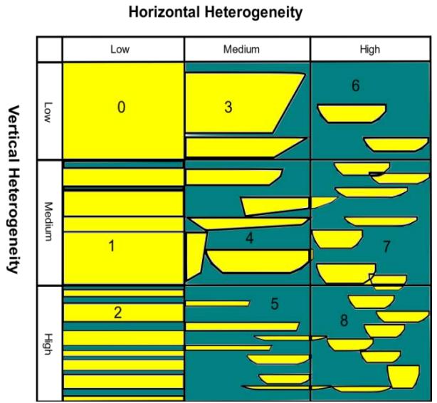 Figure 1: Depositional heterogeneity and flow unit diagram showing heterogeneity scale used for all the different Sub-environments, $0 =$ means low vertical and horizontal heterogeneity, highly connected sand reservoir with no clay or shale barriers. $8 =$ extremely heterogeneous, low net to gross reservoir sand bodies are isolated within clay or shale intervals (Modified after Tyler and Finley 1991; Aliyuda et al., 2020). Table 1: Parameters used for the study, their range and definition. <table><tr><td>Parameter</td><td>Description</td><td>Parameter range</td><td>Data source</td></tr><tr><td>Gross depositional environment</td><td>Specific environments of sediment deposition, reservoirs were classified further into Gross Depositional Environments (GDE) and Depositional-environment (DE) using the SAFARI classification Schema.</td><td>0.0 = Deep marine 0.5 Paralic/shallow marine 1 = Continental</td><td>NPD well reports, wireline logs, core images, literature</td></tr><tr><td>Diagenetic impact</td><td>Negative impact of reservoir sediments reconstitution and/or rearrangement resulting in a reduction of porosity and permeability only. It is classified into low, moderate or high impact. 0 = Low, 0.5 = Moderate, and 1 = High.</td><td>0 = Low 0.5 = Moderate 1 = High.</td><td>NPD well reports, literature</td></tr><tr><td>Stratigraphic heterogeneity</td><td>A measure of aerially extensive architecturally bounding surfaces that compartmentalize the reservoirs (after Tyler and Finley 1991). A scale of 0-8 was used with 0 = Very low heterogeneity and 8 = Extremely heterogeneous (Fig. 2.3)</td><td>0 = low vertical, low-horizontal heterogeneity 1 = low vertical, medium horizontal heterogeneity 2 = low vertical, high-horizontal heterogeneity 3 = medium vertical, low horizontal heterogeneity 4 = medium vertical, medium horizontal heterogeneity 5 = medium vertical, high horizontal heterogeneity 6 = high vertical, low horizontal heterogeneity 7 = high vertical, medium horizontal heterogeneity 8 = high vertical, high horizontal heterogeneity</td><td>NPD well reports, wireline logs, core images, literature</td></tr><tr><td>Porosity (%)</td><td>The average porosity of the reservoir interval</td><td>P10 porosity reported by field operators</td><td>NPD well reports, wireline logs, literature</td></tr><tr><td>Permeability (mD)</td><td>The average permeability of the reservoir interval</td><td>P10 permeability reported by field operators</td><td>NPD well reports, wireline logs, literature</td></tr><tr><td>Reservoir depth (m)</td><td>Highest point on reservoir units or interval</td><td></td><td>NPD well reports, literature</td></tr></table> ## III. METHODS Five machine learning algorithms were used for the study; these are Linear Regression, Support Vector Machine (SVM), Boosted Tree, Bagged Tree and Random Forest. Boosted Tree and Bagged Tree are ensembles techniques of the Decision Tree methods. Regressions are statistical technique that approximate the relationship between a dependent variable (the response) and one or more independent variables. Linear regression is mostly used for forecasting and finding out cause and response relationship between variables. Regression techniques mostly differ based on the number of independent variables and the type of relationship between the independent and dependent variables. Linear regression models are often plagued by a significant bias (Seber 1977; Mann 1987), where the predictor variables are cross correlated with each other and with the response variables, this results into the models reporting high accuracy but do not make accurate prediction of the new data. Some alternatives to linear regression are regularised linear regression approaches such as LASSO regression, Ridge regression, Elastic Net and Non-parametric regressors, usually based on decision trees. Decision tree regression takes multiple columns of potential predictor variables and finds a subset of predictor columns that best account for the variance of the target column values (Fig. 2). Boosted Decision Tree regression algorithms together with Bagged Decision Tree are ensembles of regression decision trees. In boosted regression, the algorithm learns by fitting the residual of the trees that preceded it, thereby improving accuracy with some small risk of less coverage. Bagged regression assumes a basic model structure as the one developed in a decision tree regression. Then, it divides the source data into several bags or groups and fits the same assumed model structure to each bag of data. Bagged regression aggregates the model estimates for each bag of data into one overall model. 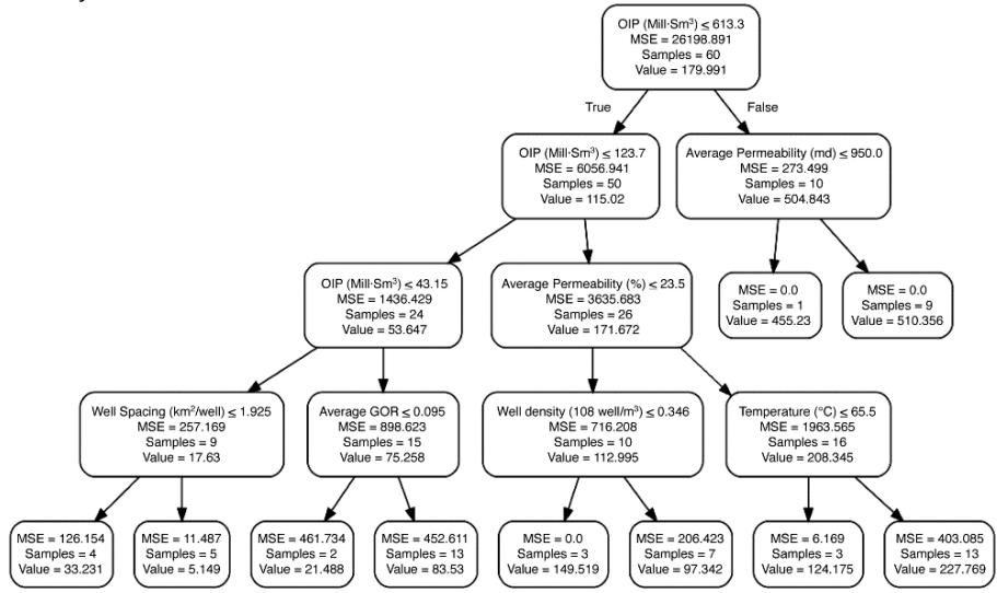 Figure 2: Decision tree regression schematic of a reservoir rate model, an example of a decision tree split at each node (Aliyuda et al., 2020). Support vector machine (SVM) is a supervised machine learning algorithm that are commonly used to analyse data characteristic of both classification and regression problems. In SVM, each of the training data points is marked as one of two categories and then iteratively builds a region that will separate the data points in the space into two groups such that the data point in each region is well separated across the boundary with the maximum width. Support vector machine can generalize the characteristics that differentiate the training data that is provided to the algorithm. This is achieved by checking for a boundary that differentiates the two classes with the maximum margin. The boundary that separates the two classes is known as a hyperplane (Cortes and Vapnik 1995; Aliyuda and Howell, 2019; Ali et al., 2021a; Ali et al., 2021b). Random forest is a common non-parametric regression approach which aggregates an ensemble of decision trees in order to arrive at a result. It predicts by taking the mean of the output from various trees. Increasing the number of trees increases the precision of the outcome. The decision trees are generated in parallel, and each split is made from random subsets of the dependent variables. Decision trees generated through taking random columns from the dependent variables are less prone to overfitting (Breiman, 2001). This technique allows random forests to be more robust than decision trees. Data for this study were normalised using min-max method, other pre-processing techniques performed on the data include a split of the data into training and testing sets. These techniques prevent against over-fitting of the models. The training set is used to train the model, whereas the testing set is used to detect the accuracy of the model and output the predicted reservoir porosity. Explained variance or R-squared (R2), square root of the mean squared error (RMSE) and mean absolute error (MAE) were used to estimate the performance and the accuracy of the trained models: $$ \mathcal{R}^{e} = \frac{N \sum x y - \sum x \sum y}{\sqrt{\left[ N \sum x^{2} - (\sum x)^{2} \right] \left[ N \sum y^{2} - (\sum y)^{2} \right]}} $$ $$ R M S E = \frac {\sqrt {\sum_ {i = 1} ^ {N} \left(y i - p i\right) ^ {2}}}{N}, \quad . \quad . \quad . \quad . \quad . \quad | | $$ $$ M A E = \frac {\sum_ {i = 1} ^ {N} | y i - p i |}{N},. \quad . \quad . \quad . \quad . \quad . \quad . \quad . \quad . \quad . \quad . \quad . \quad . \quad . $$ 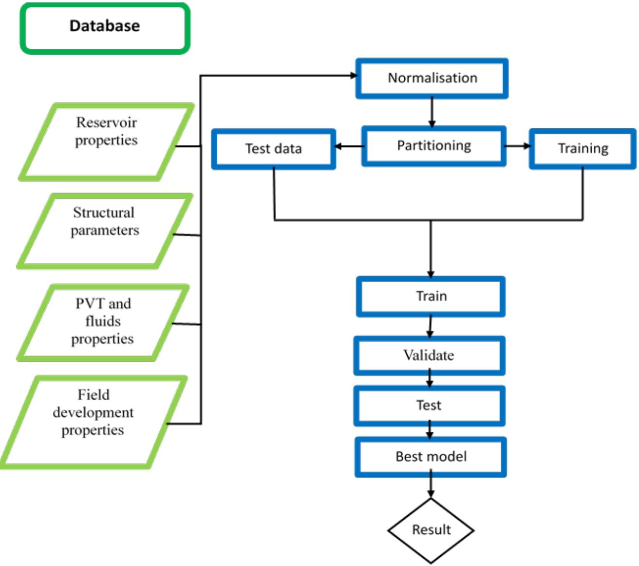 Figure 3: Workflow used to show the rundown of the procedure from building the database to training and testing of models (adopted from Aliyuda et al 2020). ## IV. RESULTS/DISCUSSION The distribution of some of the major predictors of the model is presented in Fig. 4, 5 and 6, these predictors are reservoir depth of burial (Fig. 4), gross depositional environments (Fig. 5) and reservoir stratigraphic heterogeneity (Fig. 6), as well as the response variable (Fig. 7). 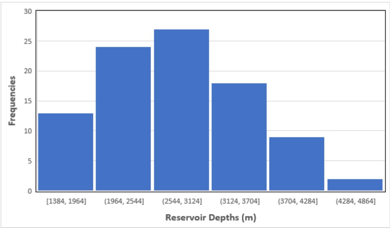 Figure 4: Distribution of reservoir depths of all the 93 reservoirs in the database. About half of the reservoirs are buried below 2,000 meters subsea. 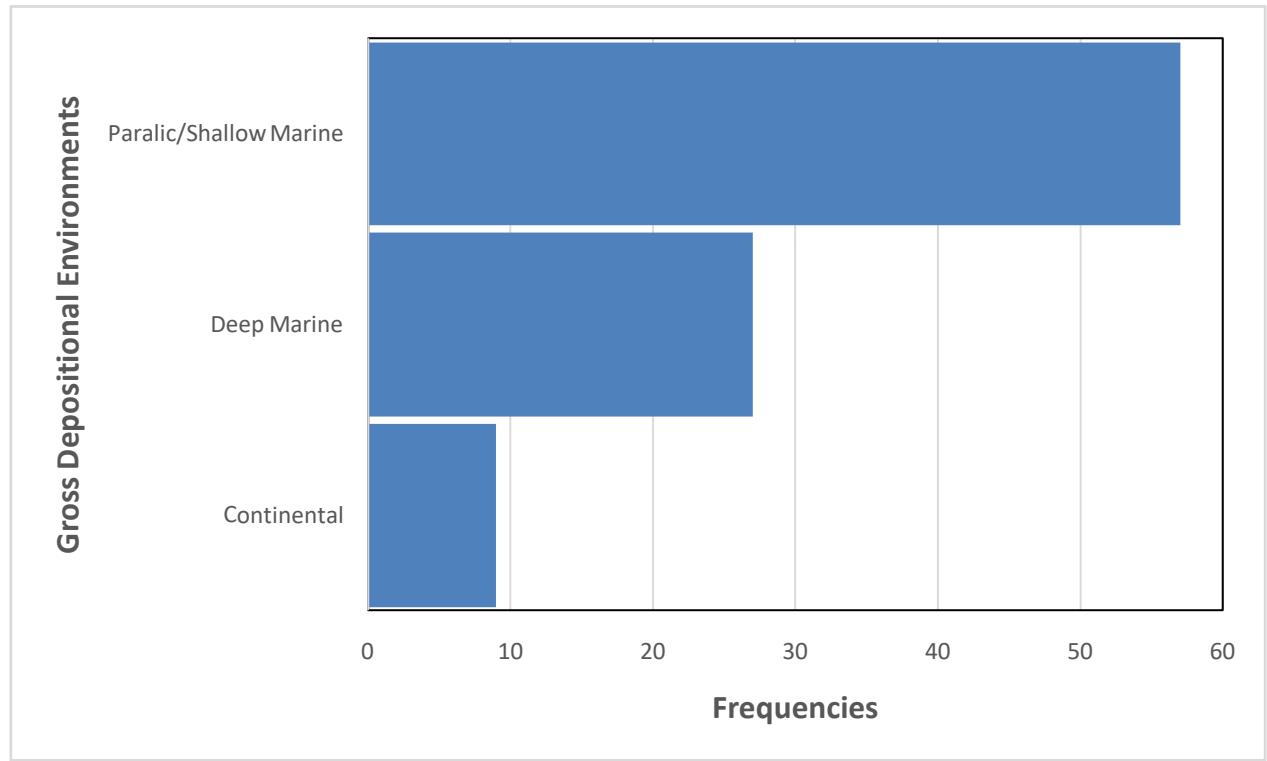 Figure 5: Proportion of the gross depositional environments of the reservoirs in the database. 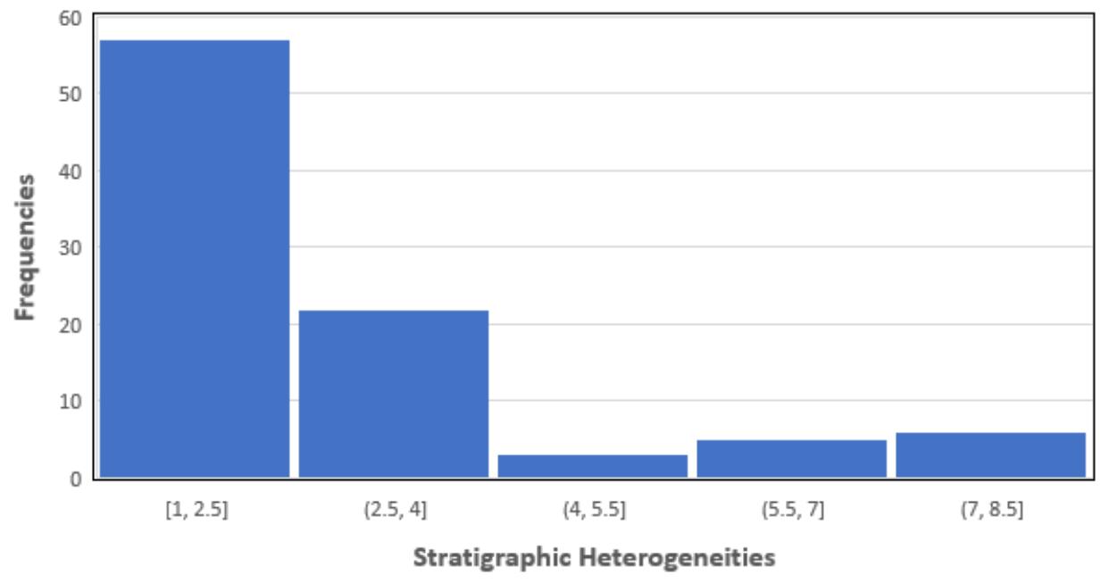 Distribution of Stratigraphic Heterogeneities Figure 6: Distribution of stratigraphic heterogeneities in the database. Low values represent low heterogeneity, high values represent high heterogeneity. 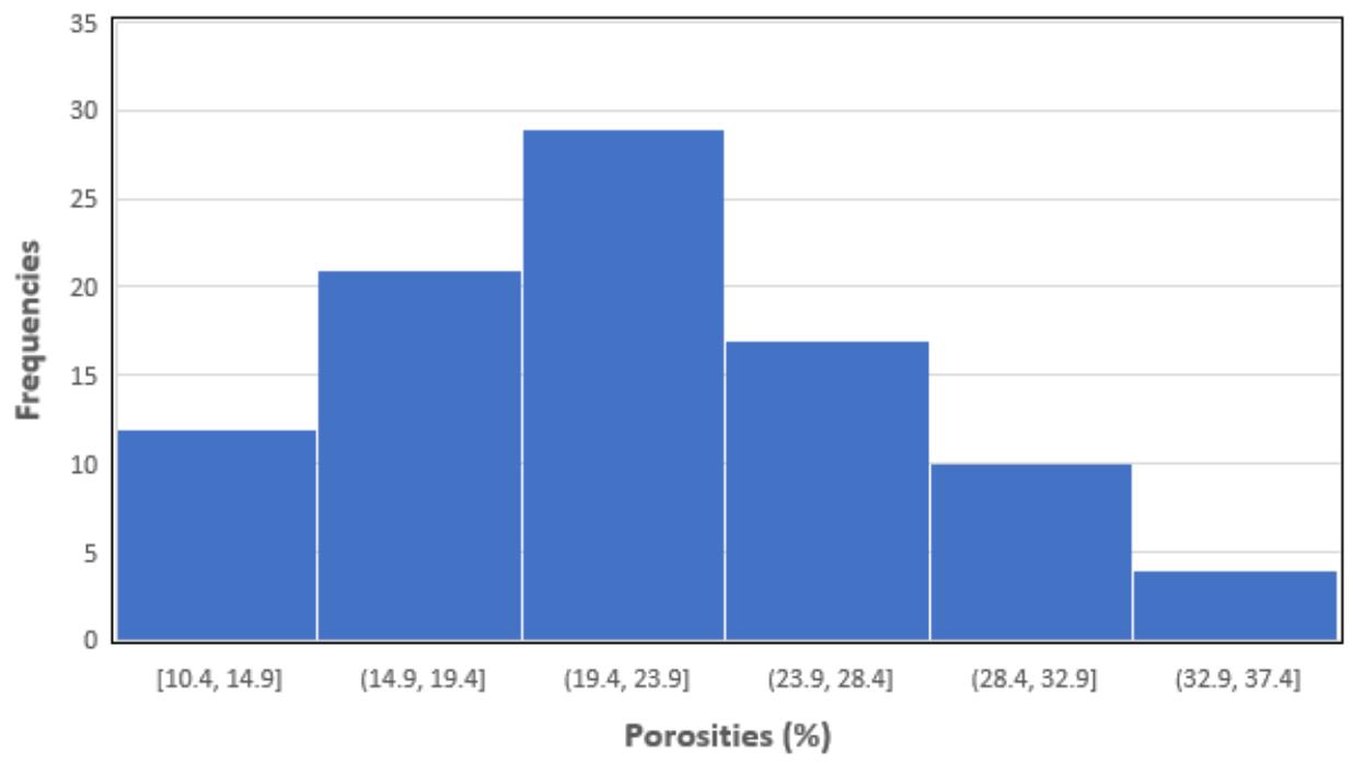 Distribution of Reservoir Porosity Figure 7: Porosity distribution of all reservoirs in the database. Reservoir porosity ranges from a minimum of $10\%$ to a maximum of $37\%$. Figures 8 and 9 demonstrate the correlation between two key predictors -reservoir depth of burial and stratigraphic heterogeneity with reservoir porosity. For the porosity against reservoir depth plot, it shows a slight decrease in porosity with increase in depth, except for a few outlier points which might indicate early migration of oil, halting reservoir porosity decline with increasing depth. The machine learning algorithms learns from these data to make prediction. The relationship between porosity and reservoir stratigraphic heterogeneity (Fig. 9) is not as strong as the one between reservoir depth and porosity (Fig. 8), the plot still shows some level of correlation between the two variables. 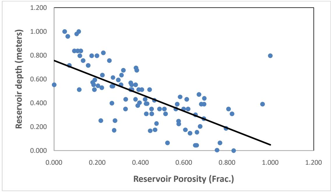 Figure 8: The relationship between reservoir depth and porosity, all measurements are in fraction (from 0 to 1). 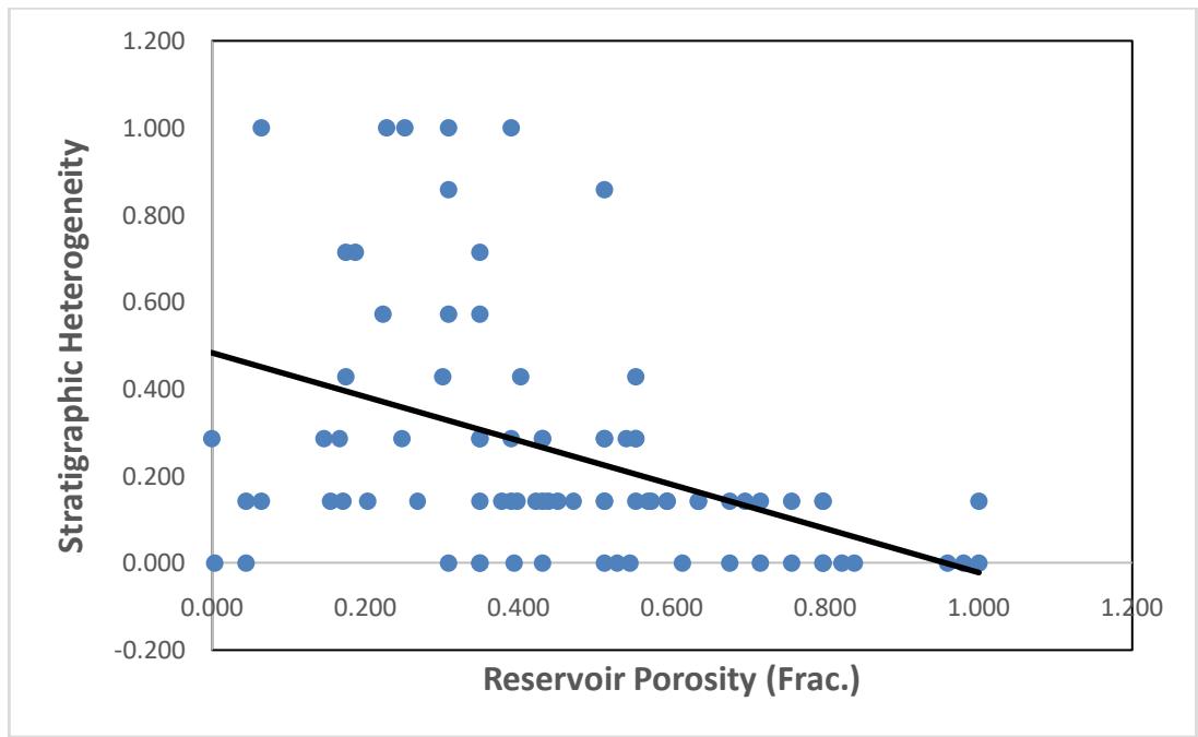 Figure 9: A plot of reservoir stratigraphic heterogeneity against porosity. Both measurements are in fraction. We trained five different models using 5 different algorithms: Linear regression; support vector machine with a Gaussian kernel function, Boosted Tree with a minimum leaf size of 8, 30 number of learners and learning rate of 0.1; Bagged Tree with minimum leaf size of 8 and 30 number of learners; random forest regression with surrogate and 200 trees. The performance of the different models was compared using three metrics (Table 2), random forest model outperformed all other models. The comparison does not include model training time as no model took up to one minute to train. Table 2: Performance of the different models trained compared using R-squared, root mean square error (RMSE) and mean absolute error (MAE). <table><tr><td>Models</td><td>R2</td><td>RMSE</td><td>MAE</td></tr><tr><td>Linear Regression</td><td>0.57</td><td>0.155</td><td>0.116</td></tr><tr><td>Support Vector Machine</td><td>0.62</td><td>0.145</td><td>0.112</td></tr><tr><td>Boosted Tree</td><td>0.52</td><td>0.163</td><td>0.128</td></tr><tr><td>Bagged Tree</td><td>0.44</td><td>0.177</td><td>0.139</td></tr><tr><td>Random Forest</td><td>0.75</td><td>0.118</td><td>0.0028</td></tr></table> 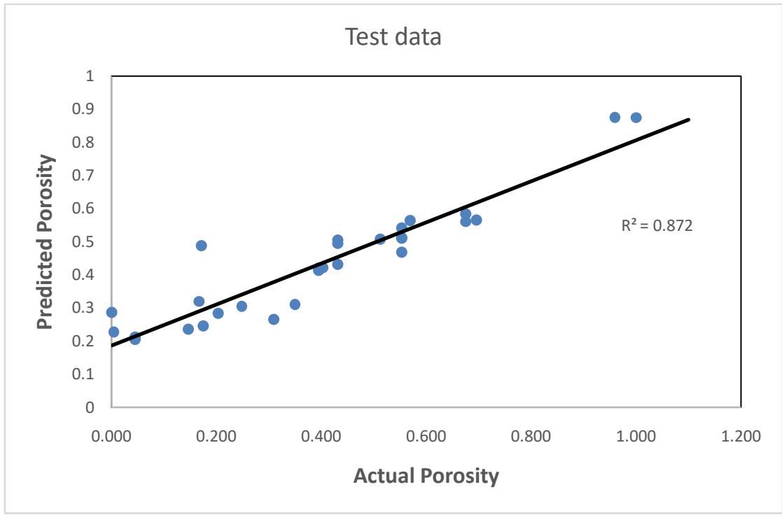Figures 10, 11 and 12 demonstrate the relationship between the predicted porosity and the actual porosity in the database for the random forest model. Fig. 12 shows a better match between the predicted porosity and the actual porosity in the test data with $R^2$ score of 0.87, compared to Fig. 10 and 11 with an $R^2$ of 0.75 and 0.71 respectively. 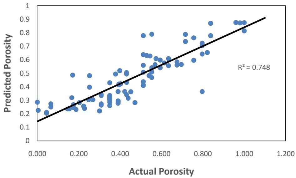 All data Figure 10: The relationship between predicted porosity and actual porosity for both training and testing data from the random forest model. 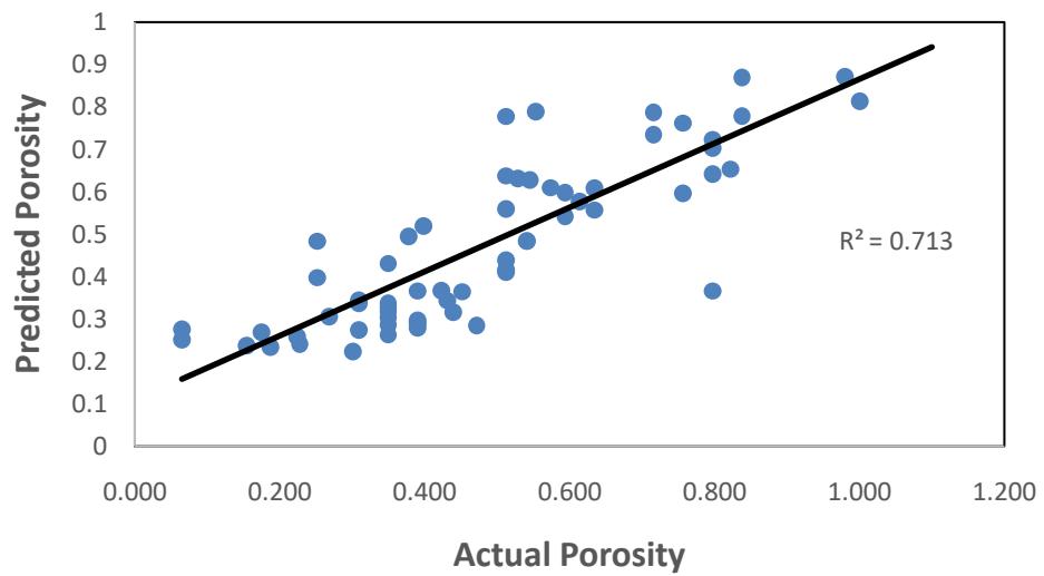 Training data Figure 11: Cross plot of actual and predicted porosity for the training data.  Figure 12: Relationship between the actual and predicted porosity for the test. ## V. CONCLUSION The machine learning technique of predicting porosity has numerous advantages over traditional techniques such as the empirical/semi-empirical formulae, Wyllie's equation and the density equation for porosity conversion where some suits of logs are used to predict porosity. The workflow shown in this study does not depend on any predetermined logs, it relays on a detailed characterization of the reservoir and its sedimentology. The machine learning approach represents a pragmatic approach to the classical log conversion problem that over the years has caused dilemmas to generations of geoscientists and petroleum engineers. The method requires no underlying mathematical models or costly assumptions of linearity among variables. Predicting porosity by using sedimentological parameters can effectively reduce the high cost of using petrophysical methods such as nuclear magnetic resonance and other logging methods. The main limitation of the method is the amount of effort required to build a robust database, preprocessed the data and partition the data into training and testing sets, which is common for all models relying on real data, and the time to train and test the models. On the other hand, once established, the application of the models requires a minimum of computing time. For the five porosity models trained, we find that models trained using random forest algorithm outperformed all the other models. The model has an R-squared score of 0.75 and MAE score of 0.0028. This study shows that machine learning has a strong potential to solve some important subsurface problems and could be an alternative to conventional methods of predicting porosity. This method can predict porosity not just around a wellbore but for some distance away from the well. ### ACKNOWLEDGMENTS The authors wish to thank the University of Aberdeen for providing the software license of MATLAB used for this study. Author Contributions Conceptualisation: Kachalla Aliyuda Data Curation: Aliyuda Ali, Kachalla Aliyuda Data Analysis: Kachalla Aliyuda, Aliyuda Ali Manuscript Writing: Kachalla Aliyuda Manuscript Review and Editing: Kachalla Aliyuda, Jerry Raymond, Aliyuda Ali, Abdulwahab Muhammed Bello Manuscript Proof-reading: Abdulwahab Muhammed Bello, Jerry Raymond Competing Interests Statement There are no financial conflicts of interest to disclose.

Generating HTML Viewer...

References

25 Cites in Article
Emilson Leite,Alexandre Vidal (2011). 3D porosity prediction from seismic inversion and neural networks.
Xian Shi,Gang Liu,Yuanfang Cheng,Liu Yang,Hailong Jiang,Lei Chen,Shu Jiang,Jian Wang (2016). Brittleness index prediction in shale gas reservoirs based on efficient network models.
Wang,S Peng,T He (2018). A novel approach to total organic carbon content prediction in shale gas reservoirs with well logs data, Tonghua Basin, China.
P Wang,S Peng (2018). A new scheme to improve the performance of artificial intelligence techniques for estimating total organic carbon from well logs.
Feisheng Feng,Pan Wang,Zhen Wei,Guanghui Jiang,Dongjing Xu,Jiqiang Zhang,Jing Zhang (2020). A New Method for Predicting the Permeability of Sandstone in Deep Reservoirs.
A Talkhestani (2015). Prediction of effective porosity from seismic attributes using locally linear model tree algorithm.
Pan Wang,Suping Peng (2019). On a new method of estimating shear wave velocity from conventional well logs.
Fusun Tut Haklidir,Mehmet Haklidir (2020). Prediction of Reservoir Temperatures Using Hydrogeochemical Data, Western Anatolia Geothermal Systems (Turkey): A Machine Learning Approach.
Ahmed Mahmoud,Salaheldin Elkatatny,Dhafer Al Shehri (2020). Application of Machine Learning in Evaluation of the Static Young’s Modulus for Sandstone Formations.
M He,H Gu,H Wan (2020). Log interpretation for lithology and fluid identification using deep neural network combined with MAHAKIL in a tight sandstone reservoir.
L Vernik (1997). Predicting porosity from acoustic velocities in siliciclastics: a new look.
Zhang Zhenhua,Yanbin Wang,Pan Wang (2011). On a Deep Learning Method of Estimating Reservoir Porosity Mathematical Problems in Engineering.
Aliyuda Ali,Kachalla Aliyuda,Muhammed Ahmed,Samuel Saleh (2021). Data-Driven Based Pressure Field Decomposition and Reconstruction for Single-Phase Flow Model.
Ahmed Ali,Aliyuda Bello,. (2021). Deep Neural Network Model for Improving Price Prediction of Natural Gas.
Aliyuda Kachalla,John Howell (2019). Machinelearning algorithm for estimating oil-recovery factor using a combination of engineering and stratigraphic dependent parameters.
Aliyuda Kachalla,John Howell,Humphrey Elliot (2020). Impact of Geological variables in controlling Oil-reservoir performance: An insight from a machine-learning technique.
Breiman Leo (2001). Random Forest.
Chen Zunde,Guo Aihua (1998). Discussion on prediction permeability of seismic data.
W Chen,J Xie,S Zu,S Gan,Y Chen (2017). Multiple-reflections noise attenuation using adaptive randomized-order empirical mode decomposition.
Cortes Corinna,Vapnik Vladimir (1995). Support-Vector Networks.
He Yan,Peng Wen,Yin Jun (2001). Permeability prediction by seismic attribute data.
C Mann (1987). Misuses of linear regression in earth sciences.
George Seber,Alan Lee (1977). Linear Regression Analysis.
Jorge Parra,Chris Hackert,Michael Bennett,Hughbert Collier (2003). Permeability and porosity images based on NMR, sonic, and seismic reflectivity: Application to a carbonate aquifer.
Explore published articles in an immersive Augmented Reality environment. Our platform converts research papers into interactive 3D books, allowing readers to view and interact with content using AR and VR compatible devices.
Your published article is automatically converted into a realistic 3D book. Flip through pages and read research papers in a more engaging and interactive format.
Our website is actively being updated, and changes may occur frequently. Please clear your browser cache if needed. For feedback or error reporting, please email [email protected]
Thank you for connecting with us. We will respond to you shortly.