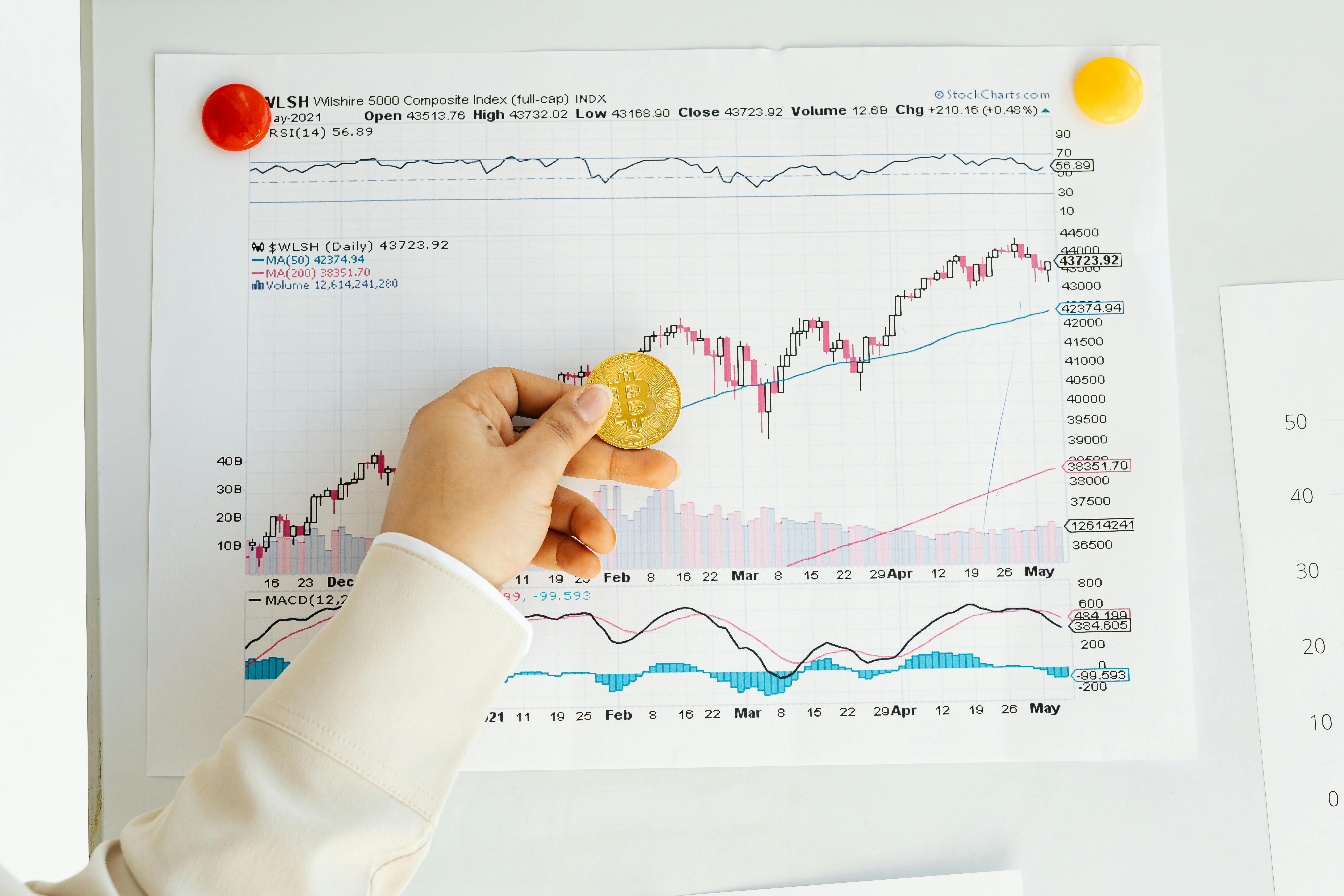
The equity market is known for its volatility and dependence on a number of factors that influence its trend. This characteristic inhibits many investors from entering this market, due to the fear of facing losses in their investments. A potential solution to this problem is to build portfolios that are neutral regarding their reference market. A neutral portfolio is constructed in such a way that its returns are obtained regardless of the trend, using automated trading systems (ATS). One of the advantages of these systems is that they carry out negotiations automatically, increasing speed and eliminating the emotional factor of manual negotiations. The proposed solution in this manuscript minimizes the correlation of portfolio returns with market index returns and uses the Walk Forward (WF) test for validation. Several portfolios are considered and the results demonstrate that in addition to being neutral, their returns exceeded the index returns. The best results were obtained for the portfolios that used a greater amount of automated strategies and made use of long/short trades.
## I. INTRODUCTION
Automated investments began in the 70's and their importance in the market increases yearly (Haynes and Roberts, 2017; Parana, 2017). It is estimated that on the New York Stock Exchange, more than $70\%$ of trades are automated through ATS (Automated Trading Systems) or EA (Expert Advisors), being used by individuals, investment fund industry, and also financial institutions (Nuti et al., 2011; Kissel, 2013). In more stable economies, due to low interest rates, financial investments are concentrated in the equity market, which can provide reasonable returns. As an example, in the US alone, more than $50\%$ of people have some investment in stocks and, in most cases, they are saving resources for their retirement (Parker and Fry, 2020). On the other hand, investment in stocks is increasingly becoming more dependent on computing resources in all its aspects due to the automation of its processes. Reinforcing this trend, ATS have the advantage of eliminating the emotional factor present in manual trading, in addition to use strategies that have already been tested and approved before being launched on the market. Studies show that investors who trade on their own in general obtain results below the market index, and, a significant part of them abandon this type of investment (Barber and Odean, 2000). Another advantage of ATS is the time saving since it is not necessary to be constantly following trades or market fluctuations. In addition, ATS can implement strategies that eliminate the factors that contribute to losses. Most manual trading strategies can be implemented automatically, eliminating the human factor. Currently, different strategies have been adopted in ATS, involving different areas, such as: computational intelligence (neural networks, genetic algorithms, machine learning, fuzzy logic, etc), technical analysis (trend followers, return to average, divergent and convergent, oscillators, etc), pattern recognition, among others (Nuti et al., 2011). However, if one of these strategies is adopted individually it can be subjected to prolonged periods of losses, known as drawdown or capital reduction. The combination of stocks in a portfolio generally contributes to the reduction of these sequences of losses (Chekhlov, Uryasev and Zabarankin, 2005). In Brazil, automation became more popular in 2014, when major brokerages started to provide platforms (Meta Trader, GrapherOC, Ninja Trader, Quantopian) with support for ATS (Folha Vitoria, 2014). It is estimated that more than $40\%$ of trading on the São Paulo Stock Exchange is carried out by ATS (Parana, 2017).
Several people are afraid of ATS, or even stock markets, due to the higher exposure to risk. In risk theory, one of the methods to deal with this situation is diversification. Harry Markowitz, Nobel laureate in Economics in 1990 for the construction of the Portfolio Theory, proposed a strategy that involves building a portfolio composed of different assets with low correlation so that individual risk can be mitigated. Markowitz defined what became known as the efficient frontier that establishes how much of each asset will be allocated in the portfolio (Markowitz, 1952). This theory has been widely used by funding industry as a way to maximize profit and minimize risk, along with its variants. An existing problem in the application of this theory stems from the fact that the correlations are not stationary and, therefore, the stability of the portfolio may vary over time, increasing risk anyway. Another type of portfolio is the neutral portfolio, which consists of a set of financial assets that, under ideal conditions, should exhibit a yield independent of the index adopted as a reference. To obtain this result, one strategy is to carry out trades in the long and short position. In the long position, the investor buys an asset in the expectation that there will be an appreciation in price (for example, shares). If this happens, the investor will make a profit after its sale. In the short position, the investor borrows an asset and sells it in the expectation that prices will fall. After the price drop, the investor buys the asset and returns it earning a profit.
In this work, the results of the implementation of an ATS portfolio neutral in relation to the Brazilian stock market index (Ibovespa) and the dollar x Brazilian real market index (USDBRL) will be presented, trading contracts on the BMF Bovespa futures market. The choice of intraday trading was made to maintain a trend away from the daily chart. In addition, another criterion adopted was the minimization of the correlation of the daily returns of the portfolios' trading with the daily returns of the Ibovespa and the USDBRL. The main contribution of this manuscript is to introduce a methodology for obtaining market neutral portfolios by minimizing the correlation of ATS portfolio returns and the benchmark index. In addition it also shows that we can build neutral ATS portfolios and that neutral portfolios can be profitable.
This article is organized as follows: Section 2 presents a review of the literature related to ATS, portfolios and neutral portfolios. In section 3, a formulation of the problem of implementing the neutral portfolio will be given for different combinations of ATS applied to the Brazilian stock market BMF Bovespa. Section 4 shows the computational results and in section 5, the conclusion is presented.
## II. LITERATURE REVIEW
The stock portfolio optimization model was proposed by Harry Markowitz (1952) in his original work "Portfolio Selection". This study supported the Modern Portfolio Theory (TMP), also known as the mean-variance model. This concept brought a revolution in the theory of finance by shifting the focus from the individual analysis of assets to diversification based on the concepts of covariance, risk, profit and their mathematical foundation. This approach seeks to identify the portfolio that provides the highest expected profit by indicating the number of shares that should be purchased for a given level of risk or the lowest possible risk for a given expected profit. Markowitz's results point to an "efficient frontier", which corresponds to a Pareto-front in the risk-return graph. One of the main elements of TMP is that risk minimization depends on the number of stocks for diversification and their low correlation.
Since TMP publication, several other portfolio optimization models have been proposed but TMP is still under use due to its ease implementation. Rosenberg et al. (2004) used the TMP to allocate portfolios with several US equity funds, for short and long-term strategies (converging and divergent), with results that contributed to decrease volatility and increase risk/reward ratio. Irala and Patil (2007) applied the TMP to the Indian stock market from 1999 to 2005 and concluded that the best diversification is obtained with a portfolio of 10 to 15 stocks for minimum risk, but recognize that this value may vary if the theory is applied in other periods. Santos and Tessari (2012) applied the TMP in several stock portfolios built from the stocks that are part of the São Paulo stock exchange index – Ibovespa. Based on different frequencies of portfolio rebalancing, they obtained statistically significant results in terms of lower volatility and risk-adjusted performance. The works by Valle et al. (2014a, 2014b, 2015, 2017) extend portfolio theory to portfolios of stocks that obtain positive returns independent of market variations.
Due to the difficulty in finding software for studying the portfolios, Prado and Bailey (2016) proposed an open-source code developed in Python that implements a version of TMP. This work contributes to the analysis of portfolio performance and the generation of its corresponding "efficient frontier". Prado (2016) also describes the instability problems of the TMP based on the fact that the correlation increases with the number of shares and develops a solution, the covariance matrix that does not need to be inverted, obtaining lower risk portfolios compared to traditional methods.
With the advances of computational intelligence, several works have been developed with the goal of optimizing stock portfolio using artificial intelligence algorithms. We can mention the use of genetic algorithms (Yang, 2006; Bao and Yang, 2008; Zainashev, 2011; Woodside-Oriakhi, Lucas and Beasley, 2011; Bermudeza, Segurab and Vercher, 2012; Mousavi, Esfahanipour and Zarandi, 2014; Wang, Hu and Dong, 2015, Jalota and Thakur, 2018) and neural networks (Freitas, Souza and Almeida, 2009; Maknickiene, 2014; Raei and Karimi, 2014) as the most prominent techniques. On the other hand, the work by Prado, Bailey and Borweiny (2016) and Raudys et al. (2016) warn about the risk of these optimizations leading to excessive parameter adjustments (overfitting) and high correlation, becoming useless in different periods. Maknickiene (2014) highlights the importance of low covariance for risk reduction, presenting the concept of orthogonality of portfolios in the Forex market. In this work, the portfolio is built from the elements that have greater orthogonality (obtained by minimizing the covariance), selected through the predictions of the distribution of returns by a neural network, resulting in greater profits for orthogonal portfolios when compared to non-orthogonal ones.
On the other hand, the movement of stock prices has been widely studied through Technical
Analysis (TA). Within this context, systems based on TA make use of indicators that are tested and used in order to define the beginning and end of a trade. This method assumes that the price of a share can follow trends according to investor psychology (Tanaka-Yamawaki; Tokuoka and Awaji, 2007). By repeating past patterns, a familiarity with the movement and behavior of prices can be developed, recognizing situations that may occur in the future. Through these patterns, different trading strategies can be implemented to be applied in different market trend situations. Lo, Mamaysky and Wang (2000) automated the identification of 10 patterns in US stock prices in the period from 1962 to 1996 and obtained promising statistical results. TA is based on three principles: the first is that price discounts everything, which allows you to disregard why prices move in a certain direction, but only to know their movement behavior. The second principle is that price has a trend. Thus, the price behaves according to the investors' position, but always obeying an uptrend, a downtrend, or having a non-trending behavior. Finally, the third principle considers that history repeats itself because the market is driven by the emotional behavior of people, who, in turn, have fears and anxieties, in a perspective of losing or winning (Murphy, 1999).
Computational intelligence has also been used to predict the movement of asset prices. Lin, Yang and Song (2011) used genetic algorithms to learn the trading rules of Technical Analysis and suggest the ideal moments for buying or selling a share. The developed system surpassed the S&P500 index of the New York Stock Exchange, in up or down trends, in the period from 2000 to 2005. Oliveira et al. (2013, 2014a, 2014b) used TA, linear regression and neural networks to trade in high-frequency trading (HFT) generating buy and sell signals for the same day in the Brazilian stock market. These systems are characterized by the high rate of volume and frequency of trades. The best results were obtained on the 5-minute time scale, which allows to send a big number of orders and increases market liquidity.
In addition to produce buy and sell signals, complete trading systems have been developed with the ability to perform all stages of the process automatically, not only generating the signals but also sending trading orders to the market and managing risk. These algorithms, that act directly on the broker's signal, are called ATS – automated trading system or EA – expert advisors (Nuti et al., 2011). Several works have been carried out for the development of ATS, considering the growing interest in the scientific/academic environment. Pimenta et al. (2017) proposed an ATS that brings a combination of genetic programming and Technical Analysis rules, applied to the Brazilian stock market from 2013 to 2016. This system was tested on the historical price series of six companies representing the Brazilian market, obtaining results higher than individual stock price changes over the same period. Neural networks are also being used for the development of automatic trading systems. Vanstone and Finnie (2009) present a methodology describing the steps involved in creating the neural network for use in the stock market and that adapts to real-world constraints. Another ATS that combines indicators from Technical Analysis was developed by Teixeira and Oliveira (2010). The strategy was applied to the Brazilian market and compared with the buy and hold (BH) method, with better results than BH in 12 of the 15 stocks analyzed in the experiment. The BH method consists of simply buying stocks of one or more companies without selling them during the entire period. The investment profit will come solely from the appreciation of the individual shares. Many strategies that involve successive purchases and sales are compared to the result of the BH method applied to the same actions in order to verify if the method brings any advantage. Creamer and Freund (2010) developed an ATS that applies machine learning, an online learning algorithm to a money management layer, which can be used with multiple market actions. One of the advantages of this approach is that the algorithm is able to select the best parameters from technical indicators. In addition, the online algorithm suggests whether to buy or sell the trade. Money management will validate whether it is possible to send the order or not. The ATS was applied to the data of 100 randomly selected stocks in the New York stock market during the period 2003 to 2005. The returns generated exceeded the market index returns.
An architecture for testing past quotes and automatic trading was proposed by Koors and Page (2011). This simulator was successful implementing simultaneous trading strategies and also making the direct connection with the real market. Ibrahim (2014) has been developing a system called GeneticForex, whose main objective is to generate strategies for an ATS portfolio with application in the Forex market. Evolutionary algorithms are used to generate several strategies but the system was not capable of eliminating redundant strategies. Among the future works is the creation of a portfolio of efficient ATS for trading with adaptive configurations in real time, where trading volumes are determined according to previous performance and that communicate with each other. Works that present studies of ATS portfolios are still rare. Treleaven, Galas and Lalchand (2013) provide an overview of the main concepts involved in the development of ATS, describe an architecture for a portfolio of different strategies and an implementation proposal. Some questions are left open, bringing numerous research perspectives to the future, such as: selection of the best computational statistics and machine learning algorithms, how news can be used to forecast market movements, ATS interaction algorithms and the market, high-performance computing and latency issues in negotiations and the use of new hardware. In this line, the works of Raudys and Raudys (2011, 2012), Raudys, Raudys and Pabarskaite (2012) and Raudys (2013) are also highlighted, who carry out the optimization of stock and HFT portfolios through the analysis of trading histories. One of the objectives of these studies is to determine what weights each ATS should have in the portfolio through the covariance matrix, using a two-stage multi-agent system for decision making. Their experimental results based on the out-sample validation methodology using the Walk-Forward steps applied to the US market from 2002 to 2012 confirm the effectiveness of the approach used, surpassing the original Markowitz model. A limitation presented in this study was the increase in the correlation of the system with the increase in the number of ATS. One challenge presented was the need to develop adaptive algorithms that take into account market changes.
Relatively few works address the implementation of neutral portfolios. With this objective, Ganesan (2011) applied the regression of the returns of individual stocks against several factors. They adopted Markowitz's (1952) mean-variance approach to portfolio development where they set the portfolio's exposure to these factors to be zero. Kwan (1999) also used a regression of stock returns against market returns, viewing the market-neutral portfolio as one where the weighted parameters of the regression in relation to the slope are equal. They formed a portfolio subject to this constraint by maximizing the Sharpe ratio indicator (1994). Pai and Michel (2012) used the regression of stock returns against market returns and viewed the neutral portfolio as one in which the weighted parameters of the regression in relation to the slope are nonlinearly related. In this work, the Markowitz mean-variance approach was also used to build a portfolio with a risk based on a nonlinear constraint. Valle (2014a) obtains neutral portfolios on a base of more than 1200 US stocks and a model based on minimizing the correlation of portfolio returns and S&P500 index, with results that outperform the regression-based approach with long and shorts.
## III. PROBLEM
### a) Presentation
A neutral portfolio is a portfolio that ideally has zero correlation with the market. In order to define which These variables are defined by the expressions:
ATS will be part of this portfolio, we adopted the nonlinear model proposed by Valle (2014a), which minimizes the correlation of the returns of the ATS portfolio in relation to the returns of the reference market will be applied.
In sequence, the notation, constraints, and objective function considered are presented. The model uses trades generated by the trading strategies of intraday and daily long and long/short contracts on the BMF Bovespa future market.
### b) Notation
Given the returns of the $N$ ATS strategies and $T$ time intervals $0,1,2,\ldots,T$, the goal is to select the best set of $K$ strategies (where $K <= N$ ), and their weights.
Let:
I indexes the portfolios
$T$ indexes the time intervals
Vit is the value/margin (price) of a contract $i$ at time $t$ $lpit$ is the profit/loss of strategy $i$ at time $t$
$C_t$ is the value of portfolio capital at time $t = 0, \dots, T$
$C_{o}$ is the net capital of the portfolio at time $t = 0$
It is lbovespa value at time $t$
$R_{t}$ is one-period return for the Ibovespa at time $t$ i.e. $R_{t} = \ln (I_{t} / I_{t - 1})$
$\bar{R}$ is the average index return, ie $\bar{R} = \sum_{t=1}^{T} \frac{R_t}{T}$
#### The decision variables are:
$x^{L}{}_{i}, x^{S}{}_{i}$ the number of units $(>=0)$ of strategies that will be held in long or short positions. In our approach, the integer constraint is relaxed and the continuous values are rounded to the closest integer value. Although this strategy is not optimal, it suitable to approximate problem solutions (Hillier and Lieberman, 2015), with polynomial computational complexity.
### c) Objective Function
According to the definition adopted, the neutral portfolio must maintain a correlation between its returns and the return of the index equal to or close to zero. The correlation result is comprised within a closed interval $[-1, +1]$. For the definition of the model, the following additional variables will be defined:
$p_t$ neutral portfolio log return at time $t = 1, \ldots, T$ $\mathsf{p}^-$ neutral portfolio average return
$$
C _ {t} = \mathrm {C} _ {\mathrm {o}} + \sum_ {i = 1} ^ {K} x _ {i} ^ {L} V _ {i t} + \sum_ {i = 1} ^ {K} x _ {i} ^ {S} V _ {i t,} + \sum_ {i = 1} ^ {K} x _ {i} ^ {L} l p _ {i t} + \sum_ {i = 1} ^ {K} x _ {i} ^ {S} l p _ {i t,}, \quad t = 0, \dots , T \tag {1}
$$
$$
p _ {t} = \ln \left(C _ {t} / C _ {t - 1}\right), \quad t = 1, \dots , T
$$
$$
\bar{\mathbf{p}} = \sum_{t=1}^{T} p_{t} / T
$$
The eq. (1) demonstrates that at a given time the portfolio has a part of the capital $\sum K_{i=1}^{K} x^{L} i V_{it}$ in long positions and the other part $\sum K_{i=1}^{K} x^{S} i V_{it}$, in short positions, a net available capital $C_{0}$ and a floating part $\sum K_{i=1}^{K} x^{L} i l p_{it} + \sum K_{i=1}^{K} x^{S} i l p_{it}$, related to profits/losses. The eq. (2) defines the log-returns and eq. (3) to the average return.
In the model adopted to obtain the neutral portfolio, the objective is to minimize the correlation between the daily return of the portfolio and the daily return of the indices. This operation can be defined by the expression (4):
$$
\text{minimize} \left| \frac{\sum_ {t = 1} ^ {T} \left(p _ {t} - \bar{p}\right) \left(R _ {t} - \bar{R}\right)}{\sqrt{\sum_ {t = 1} ^ {T} \left(p _ {t} - \bar{p}\right) ^ {2} \sum_ {t = 1} ^ {T} \left(R _ {t} - \bar{R}\right) ^ {2}}} \right| \tag{4}
$$
This minimization is subject to the constraints given in Eqs. (1-3).
### d) Constraint on In-sample Returns
The model presented aims to obtain zero correlation between the return of the portfolio and in relation to the return of the index, but it does not intend to guarantee profit or exceed the return of the index in the period. To improve the results of the portfolio's in-sample return (which will not necessarily guarantee out-sample returns), the following constraint can be added:
$$
\bar {p} \geq \bar {R} \tag {5}
$$
This constraint ensures that the average return on the portfolio will be at least equal to the index return.
## IV. COMPUTATIONAL RESULTS
In this section, the computational results for performing the calculations applied to the returns of neutral portfolios will be presented. The algorithm was executed in a MacBook Air computer with an Intel Core i5 processor, 1.7 GHz, with 4 GB of RAM, with MacOS. The code was written in Python, using the Jupiter Notebook platform. The Python language is opensource and has several libraries for statistical treatment and finance (Seabold and Perktold, 2010), which motivates this use. The function corr from the Pandas library was used to calculate the correlation by Pearson's method and the minimize function from the SciPy library was used to perform the minimization, according to(4) and subject to the constraint(5) in some cases.
### a) Data and Methodologies
In this work, historical data from 30 ATS based on TA (oscillators and trend following), developed by company Metarobôs were considered, Such a data covers the period from January 2015 to December 2018. The data mostly correspond to intraday (day trade) and daily trades, with each trade involving two mini-contracts of the BMF Bovespa (WIN) or dollar (WDO) index. The history corresponds to a total of 18,609 trades. This data was chosen because it was generated using a known and reliable trading strategies (white box).
The methodology adopted for the analysis is known as Walk Forward, developed by Robert Pardo (Pardo, 2008). It involves optimizing a portfolio in a period, called in-sample (IS), and applying the optimal solution obtained to the out-sample (OS) set. Fig. 1 represents the IS intervals in yellow and the OS intervals in green.
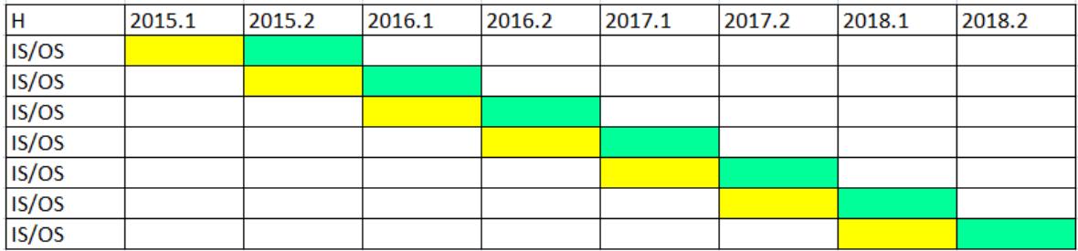 Fig. 1: Periods for the Walk Forward methodology
Initially, the interval of $H = 6$ months was adopted for both IS and OS. The value of $C = 100,000.00$ was considered for the initial capital. For each period, the daily returns of the portfolio, obtained through trades of the different daytrade and daily strategies, are accounted for. These returns are compared to Ibovespa's daily returns to minimize correlation. The minimization result applied to the IS history will define the new weights to be applied to the IS and OS period history strategies. The analysis also involves the composition of portfolios with only long trades, only trades with WDO contracts, and only trades with WIN contracts. A comparison of the results of the indices with the ATS portfolios, without optimization, was also made.
### b) Results without Optimization
Tables 1 and 2 shows the results of ATS trades without optimization, using only TA, for three portfolios. The first involves all 30 strategies (16 of WIN and 14 of WDO), the second with only 16 of WIN and the third with 14 strategies of WDO. The first two were compared with the Ibovespa and the third with the USDBRL. The three portfolios were analyzed based on long and long/short trades. For this analysis, the WF methodology was not applied, since there was no optimization. Each trade always involved two contracts (WDO or WIN) and the objective was to compare the results of the combined strategies with their respective indices.
Correlation results indicate that long portfolios with fewer strategies have positive correlation with their respective indices. The correlation is close to zero when it involves the 30 strategies in the three long/short portfolios. It indicates that with the increase of different strategies in the portfolios and the addition of short operations, the correlation with the market tends to decrease. In all portfolios, there was excess return in relation to the index, lower volatility and higher value for the Sharpe ratio (return/standard deviation ratio). These results demonstrate that ATS strategies were more profitable than market indices, presenting a better return vs. risk ratio. This form of diversification already guarantees independence from the market. In the next sections, correlation minimization will be used to define the weights of strategies in portfolios.
Table 1: Summary of results without optimization – Long (H = 6)
<table><tr><td>Index</td><td>Portfolio (N)</td><td>Correlation</td><td>Return</td><td>Excess</td><td>vol. Port.</td><td>vol. Index</td><td>Sharpe Port.</td><td>Sharpe Ind.</td></tr><tr><td>Ibov</td><td>16WIN-14WDO</td><td>0,09</td><td>0,32</td><td>0,18</td><td>0,01</td><td>0,05</td><td>6,3</td><td>2,8</td></tr><tr><td>Ibov</td><td>16WIN</td><td>0,5</td><td>0,19</td><td>0,05</td><td>0,01</td><td>0,05</td><td>3,7</td><td>2,8</td></tr><tr><td>USDBRL</td><td>14WDO</td><td>0,44</td><td>0,23</td><td>0,17</td><td>0,02</td><td>0,03</td><td>7,9</td><td>2,0</td></tr><tr><td></td><td>average</td><td>0,34</td><td>0,25</td><td>0,13</td><td>0,01</td><td>0,04</td><td>5,97</td><td>2,53</td></tr></table>
Table 2: Summary of results without optimization - Long/Short (H = 6)
<table><tr><td>Index</td><td>Portfolio (N)</td><td>Correlation</td><td>Return</td><td>Excess</td><td>vol. Port.</td><td>vol. Index</td><td>Sharpe Port.</td><td>Sharpe Ind.</td></tr><tr><td>Ibov</td><td>16WIN-14WDO</td><td>-0,03</td><td>0,5</td><td>0,36</td><td>0,02</td><td>0,05</td><td>10,0</td><td>2,8</td></tr><tr><td>Ibov</td><td>16WIN</td><td>-0,04</td><td>0,34</td><td>0,2</td><td>0,01</td><td>0,05</td><td>6,8</td><td>2,8</td></tr><tr><td>USDBRL</td><td>14WDO</td><td>-0,04</td><td>0,36</td><td>0,3</td><td>0,02</td><td>0,03</td><td>12,0</td><td>2,0</td></tr><tr><td></td><td>average</td><td>-0,08</td><td>0,4</td><td>0,29</td><td>0,02</td><td>0,04</td><td>9,6</td><td>2,53</td></tr></table>
### c) Out-sample Results
Tables 03 and 04 shows the OS results for two conditions, long and long/short respectively, for each analyzed portfolio. The correlation column provides the average correlations obtained in the seven applications of the WF method. The same applies to the Return, Excess, Volatility and Sharpe Ratio columns. The Excess column indicates how much the OS optimized portfolio outperformed the index average. Volatility is given by the standard deviation of the returns and the Sharpe ratio is obtained by the return/standard deviation ratio. In the last line, the average of each column is presented.
The most significant results in this modeling are those obtained in the OS simulation, since the IS results are only intended to obtain the weights that minimize the correlation in order to be applied in the OS intervals.
Comparing the non-optimized results (Tables 01 and 02) with the optimized OS results (Tables 03 and 04), it is observed that the values optimized achieved a reduction achieved a reduction in the average correlation from 0.34 to 0.14 for the long data and for the long/short data it remained practically stable close to zero, that is, without correlation in relation to the indices. It can be seen that long/short trades have lower correlation averages compared to long trades. This demonstrates that this combination of trades contributes to increasing the neutrality of the portfolio in relation to the market. Analyzing the returns, it is observed that the average excess of the long portfolios increased from 0,13 to 0.46 and for the long/short portfolios from 0.29 to 1.03. Taking into account the number of strategies in each portfolio, the WIN only portfolio has 16 strategies, the WDO portfolio has 14 strategies, and the WINWDO portfolio has 30 strategies. When analyzing the influence of the number of strategies, it is observed that the portfolio with more strategies WINWDO obtained higher excess return and lower correlation in relation to the indices than the other portfolios with fewer strategies. This occurs both with long trades and also with long/short trades. These results show that the best results are obtained by increasing the diversity of strategies, including long/short operation. Also, all OS portfolios achieved a decrease in correlation and an increase in Sharpe compared to the respective portfolios without optimization.
Table 3: Summary of out-sample results - Long (H = 6)
<table><tr><td>Index</td><td>Portfolio (N)</td><td>Correlation</td><td>Return</td><td>Excess</td><td>vol. Port.</td><td>vol. Index</td><td>Sharpe Port.</td><td>Sharpe Ind.</td></tr><tr><td>Ibov</td><td>16WIN-14WDO</td><td>0.03</td><td>0.81</td><td>0.66</td><td>0.13</td><td>0.05</td><td>15.9</td><td>2.8</td></tr><tr><td>Ibov</td><td>16 WIN</td><td>0.22</td><td>0.2</td><td>0.06</td><td>0.13</td><td>0.05</td><td>3.9</td><td>2.8</td></tr><tr><td>USDBRL</td><td>14WDO</td><td>0.17</td><td>0.7</td><td>0.65</td><td>5.26</td><td>0.03</td><td>25.0</td><td>2.0</td></tr><tr><td></td><td>average</td><td>0.14</td><td>0.57</td><td>0.46</td><td>1,84</td><td>0.04</td><td>14,9</td><td>2.5</td></tr></table>
Table 4: Summary of out-sample results - Long/Short (H = 6)
<table><tr><td>Index</td><td>Portfolio (N)</td><td>Correlation</td><td>Return</td><td>Excess</td><td>vol. Port.</td><td>vol. Index</td><td>Sharpe Port.</td><td>Sharpe Ind.</td></tr><tr><td>Ibov</td><td>16WIN-14WDO</td><td>-0.03</td><td>1.25</td><td>1.11</td><td>0.15</td><td>0.05</td><td>24.5</td><td>2.8</td></tr><tr><td>Ibov</td><td>16 WIN</td><td>0.02</td><td>1.18</td><td>1.04</td><td>0.21</td><td>0.05</td><td>23.6</td><td>2.8</td></tr><tr><td>USDBRL</td><td>14WDO</td><td>-0.04</td><td>1</td><td>0.94</td><td>0.2</td><td>0.03</td><td>35.7</td><td>2.0</td></tr><tr><td></td><td>average</td><td>-0.02</td><td>1.14</td><td>1.03</td><td>0.19</td><td>0.04</td><td>27,93</td><td>2.5</td></tr></table>
### d) Variations
Tables 5 and 6 consider the effect of including additional variations in the portfolio in the IS optimization to examine their reflections on the OS results. The constraint (5) was included in the IS period and the H interval was also reduced from 6 to 3 months. $N = 30$ (16 WIN and 14 WDO) was maintained for the number of strategies in the portfolios, with no comparison being made with the USDBRL index, only with the Ibovespa index. Since the IS periods are intended for optimization, only the OS results will be analyzed, in tables 5 and 6.
Adding constraint (5) with $H =$ decreased the return index in the long/short portfolio but an increase in the excess in the long portfolio. On the other hand, decreasing the periods $H$ to 3, there is an increase in excess return, Sharpe ratio, and volatility, in the long and long/short portfolios. The correlation increased in the long portfolio and remained close to zero in the long/short portfolio. Such results suggest that the narrowing of the WF range better captures short-lived market patterns.
Table 5: Summary of out-sample results - Long - N = 30
<table><tr><td>Index</td><td>Correlation</td><td>Return</td><td>Excess</td><td>vol. Port.</td><td>vol. Index</td><td>Sharpe Port.</td><td>Sharpe Ind.</td><td>H</td><td>Restriction</td></tr><tr><td>Ibov</td><td>0.03</td><td>0.81</td><td>0.66</td><td>0.13</td><td>0.05</td><td>15.9</td><td>2.4</td><td>6</td><td></td></tr><tr><td>Ibov</td><td>0.03</td><td>0.99</td><td>0.85</td><td>0.13</td><td>0.05</td><td>19.4</td><td>2.4</td><td>6</td><td>p-≥ R</td></tr><tr><td>Ibov</td><td>0.15</td><td>1.05</td><td>0.9</td><td>0.25</td><td>0.05</td><td>21.4</td><td>2.4</td><td>3</td><td>p-≥ R</td></tr></table>
Table 6: Summary of out-sample results – Long/Short
<table><tr><td>Index</td><td>Correlation</td><td>Return</td><td>Excess</td><td>vol. Port.</td><td>vol. Index</td><td>Sharpe Port.</td><td>Sharpe Ind.</td><td>H</td><td>Restriction</td></tr><tr><td>Ibov</td><td>-0.03</td><td>1.25</td><td>1.11</td><td>0.15</td><td>0.05</td><td>24.51</td><td>2.4</td><td>6</td><td></td></tr><tr><td>Ibov</td><td>-0.02</td><td>1.05</td><td>0.9</td><td>0.13</td><td>0.05</td><td>21.0</td><td>2.4</td><td>6</td><td>p-≥ R</td></tr><tr><td>Ibov</td><td>-0.02</td><td>2.3</td><td>2.16</td><td>0.66</td><td>0.05</td><td>46.9</td><td>2.4</td><td>3</td><td>p-≥ R</td></tr></table>
## V. CONCLUSIONS
This work addressed the problem of implementing a neutral portfolio in relation to the BMF Bovespa market, using 30 trading strategies carried out by ATS in intraday and daily operations, in long and long/short positions. The model performs the minimization of the correlation of the daily returns in the IS period to obtain the weights of the strategies that will be applied in the OS period.
The strategies adopted are based on Technical Analysis and applied in the BMF Bovespa future market, trading Ibov index and dollar mini-contracts (WIN and WDO). The IS results obtained correlations close to zero in most cases in relation to their indexes and when applied in the OS period, an increase in the correlation was noted for long portfolios but close to zero in the long/short portfolios. In all OS portfolio combinations, returns outperformed the index.
The results indicate that it is possible to obtain neutral portfolios by combining several ATS, proving to be an alternative option in relation to the funds available in the market. The model can be improved by adding more ATS to the portfolio with different strategies and involving other markets.
Statements & Declarations
Funding
The authors declare that no funds, grants, or other support were received during the preparation of this manuscript.
Competing Interests
The authors have no relevant financial or non-financial interests to disclose.
Author Contributions
All authors contributed to the study conception and design. Material preparation, data collection and analysis were performed by Carlos A. Rodrigues. The first draft of the manuscript was written by Carlos A. Rodrigues and both authors commented and revised it critically for important intellectual content on previous versions of the manuscript. Both authors read and approved the final manuscript.
Data Availability
The data that support the findings of this study are available from Metarobos but restrictions apply to the availability of these data, which were used under license for the current study, and so are not publicly available. Data are however available from the authors upon reasonable request and with permission of Metarobos. Additionally, we cannot apply an open licence to our dataset.
Generating HTML Viewer...
References
56 Cites in Article
Depei Bao,Zehong Yang (2008). Intelligent stock trading system by turning point confirming and probabilistic reasoning.
Brad Barber,Terrance Odean (2000). Trading is Hazardous to Your Wealth: The Common Stock Investment Performance of Individual Investors.
K Parker,R Fry (2020). More than half of U.S. households have some investment in the stock market.
J Bermúdez,J Segura,E Vercher (2012). A multi-objective genetic algorithm for cardinality constrained fuzzy portfolio selection.
A Chekhlov,S Uryasev,M Zabarankin (2005). Drawdown measure in portfolio optimization.
Germán Creamer,Yoav Freund (2010). Automated trading with boosting and expert weighting.
Folha Vitória (2014). Robô russo chega ao Espírito Santo e promete mais lucro nos investimentos.
Fabio Freitas,Alberto De Souza,Ailson De Almeida (2009). Prediction-based portfolio optimization model using neural networks.
Girish Ganesan (2011). A Subspace Approach to Portfolio Analysis.
Frederick Hillier,Gerald Lieberman (2015). Introduction to Operation Research.
Alaa Ibrahim (2014). Evolutionary Approach to Forex Expert Advisor Generation.
L Irala,P Patil (2007). Portfolio size and diversification.
Hemant Jalota,Manoj Thakur (2018). Genetic algorithm designed for solving portfolio optimization problems subjected to cardinality constraint.
R Kissell (2013). Multi-Asset Risk Modeling: Techniques for a Global Economy in an Electronic and Algorithmic Trading Era.
Arne Koors,Bernd Page (2011). A Hierarchical Simulation Based Software Architecture For Back-Testing And Automated Trading.
C Kwan (1999). A note on market-neutral portfolio selection.
Xiaowei Lin,Zehong Yang,Yixu Song (2011). Intelligent stock trading system based on improved technical analysis and Echo State Network.
Andrew Lo,Harry Mamaysky,Jiang Wang (2000). Foundations of Technical Analysis: Computational Algorithms, Statistical Inference, and Empirical Implementation.
N Maknickiene (2014). Selection of Orthogonal Investment Portfolio Using Evolino RNN Trading Model.
Harry Markowitz (1952). Portfolio Selection.
Somayeh Mousavi,Akbar Esfahanipour,Mohammad Zarandi (2014). A novel approach to dynamic portfolio trading system using multitree genetic programming.
J Murphy (1999). Futures fund performance: A test of the effectiveness of technical analysis.
Giuseppe Nuti,Mahnoosh Mirghaemi,Philip Treleaven,Chaiyakorn Yingsaeree (2011). Algorithmic Trading.
H Oliveira,J Macedo,L Camargo,L Silva,R Salgado (2013). An intelligent decision support system to investment in the stock market.
H Oliveira,E B; Jabbur,A Pereira,D Castilho,E Silva (2014). Design and evaluation of automatic agents for stock market intraday trading.
H Oliveira,E B; Silva,D Castilho,A Pereira (2014). A neural network based approach to support the market making strategies in highfrequency trading.
G Pai,T Michel (2012). Differential evolution based optimization of risk budgeted equity market neutral portfolios.
E Paraná (2017). Boletim de Economia e Política Internacional.
R Pardo (2011). The Evaluation and Optimization of Trading Strategies.
Alexandre Pimenta,Ciniro Nametala,Frederico Guimarães,Eduardo Carrano (2017). An Automated Investing Method for Stock Market Based on Multiobjective Genetic Programming.
M Prado (2016). Building diversified portfolios that outperform out-of-sample.
M Prado,D Bailey (2016). An open-source implementation of the critical-line algorithm for portfolio optimization.
M Prado,D Bailey,J Borweiny (2016). Stock portfolio design and backtest overfitting.
Reza Raei,Paria Karimi (2014). Asset management using an extended Markowitz theorem.
Sarunas Raudys,Aistis Raudys (2011). High frequency trading portfolio optimisation: Integration of financial and human factors.
Sarunas Raudys,Aistis Raudys,Zidrina Pabarskaite (2012). Multi-agent system based portfolio management in prior-to-crisis and crisis period.
Sarunas Raudys (2013). Portfolio of Automated Trading Systems: Complexity and Learning Set Size Issues.
Sarunas Raudys,Aistis Raudys (2012). Three decision making levels in portfolio management.
S Raudys,A Raudys,Z Pabarskaite,G Biziuleviciene (2016). Portfolio inputs selection from imprecise training data.
M Rosenberg,J Tomeo,S Chung (2004). Hedge fund-of-funds asset allocation using a convergent and divergent strategy approach.
André Santos,Cristina Tessari (2012). Técnicas Quantitativas de Otimização de Carteiras Aplicadas ao Mercado de Ações Brasileiro.
Skipper Seabold,Josef Perktold (2010). Statsmodels: Econometric and Statistical Modeling with Python.
William Sharpe (1994). The Sharpe Ratio.
Mieko Tanaka-Yamawaki,Seiji Tokuoka,Keita Awaji (2009). Short-Term Price Prediction and the Selection of Indicators.
Lamartine Teixeira,Adriano De Oliveira (2010). A method for automatic stock trading combining technical analysis and nearest neighbor classification.
Philip Treleaven,Michal Galas,Vidhi Lalchand (2013). Algorithmic trading review.
C Valle,N Meade,J Beasley (2014). Market neutral portfolios.
C Valle,N Meade,J Beasley (2014). Absolute return portfolios.
C Valle,N Meade,J Beasley (2015). Factor neutral portfolios.
Cristiano Valle,Diana Roman,Gautam Mitra (2017). Novel approaches for portfolio construction using second order stochastic dominance.
Bruce Vanstone,Gavin Finnie (2009). An empirical methodology for developing stockmarket trading systems using artificial neural networks.
M Woodside-Oriakhi,C Lucas,J Beasley (2011). Heuristic algorithms for the cardinality constrained efficient frontier.
Weijia Wang,Jie Hu,Ning Dong (2015). A Convex-Risk-Measure Based Model and Genetic Algorithm for Portfolio Selection.
Xiaolou Yang (2006). Improving Portfolio Efficiency: A Genetic Algorithm Approach.
T Zainashev (2011). Screen confronting Two-Pair Primers from typical Genetic Algorithm to improved local search-based Genetic Algorithm.
No ethics committee approval was required for this article type.
Data Availability
Not applicable for this article.
How to Cite This Article
Carlos Alberto Rodrigues. 2026. \u201cMarket-Neutral Portfolios: A Solution Based on Automated Strategies\u201d. Global Journal of Research in Engineering - F: Electrical & Electronic GJRE-F Volume 23 (GJRE Volume 23 Issue F1): .
Explore published articles in an immersive Augmented Reality environment. Our platform converts research papers into interactive 3D books, allowing readers to view and interact with content using AR and VR compatible devices.
Your published article is automatically converted into a realistic 3D book. Flip through pages and read research papers in a more engaging and interactive format.
The equity market is known for its volatility and dependence on a number of factors that influence its trend. This characteristic inhibits many investors from entering this market, due to the fear of facing losses in their investments. A potential solution to this problem is to build portfolios that are neutral regarding their reference market. A neutral portfolio is constructed in such a way that its returns are obtained regardless of the trend, using automated trading systems (ATS). One of the advantages of these systems is that they carry out negotiations automatically, increasing speed and eliminating the emotional factor of manual negotiations. The proposed solution in this manuscript minimizes the correlation of portfolio returns with market index returns and uses the Walk Forward (WF) test for validation. Several portfolios are considered and the results demonstrate that in addition to being neutral, their returns exceeded the index returns. The best results were obtained for the portfolios that used a greater amount of automated strategies and made use of long/short trades.
Our website is actively being updated, and changes may occur frequently. Please clear your browser cache if needed. For feedback or error reporting, please email [email protected]
Thank you for connecting with us. We will respond to you shortly.