### INTRODUCTION Technically, orbital debris has been well defined in the space community. In addition, the community recognizes that orbital debris places safety and technical constraints on space operations. While researchers are studying how orbital debris affects the sustainability of commonly used Earth orbits, interest in an economic perspective on the problem is growing. Furthermore, the space engineering community is curious about the financial requirements for preserving space orbitals through debris mitigation and remediation. The OECD published comprehensive economic research on the cost of space debris in 2020 [2]. Since 1979, the Orbital Debris Program Office (ODPO) of the United States Space Agency (NASA) has also conducted some well-known studies on the assessment of orbital debris impact and preservation measures for useful Earth orbits. This study employs a different methodology to monetize the costs of orbital debris than the 2023 NASA study (Colvin et al., 2023) [15]. This study estimates the costs of space preservation by using reliable data points and assigning values to NASA-published space debris mitigation models. Monetizing the rising costs of space debris and the costs of dealing with the problem provides policymakers and the space industry with a quantifiable metric for understanding the economic nature of orbital debris. In space engineering terms, mitigation measure refers to actions of post-mission disposal (PMD) to prevent further orbital debris generation; remediation measure means actions of active debris removal (ADR) of defunct man-made objects generated in past space operations. Both measures preserve useful Earth orbits. #### Method of Break-Even Analysis The break-even point (BEP) is the point at which expenditure equals revenue. The break-even analysis method is frequently applied to an investment decision process, which can reveal whether and when the investment benefit will cover its cost given a price and quantity in its future timeline. This method is used in government regulatory analyses to determine when regulatory costs will be offset by public benefits from a finalized regulation. The concept of BEP is used in this paper, where the cost stream of preserving orbital space meets the cost stream of extending orbital debris proliferation. As a result, this break-even analysis method examines two cost streams, one of which is expected to reduce the other in the long run. In this case, the cost of space preservation can be viewed as an investment stream created to prevent the initial cost of orbital debris from spiraling upward. This method allows the study to emphasize the prospective costs of orbital debris, which are future costs that can be avoided or reduced if a corrective action is taken. This BEP analysis also identifies the global cost savings after the costs of space debris equal the costs of space preservation by conducting a break-even analysis of these cost streams. This kind of evaluation performs sensitivity analyses with alternative inputs to determine the effectiveness of mitigation and remediation options. 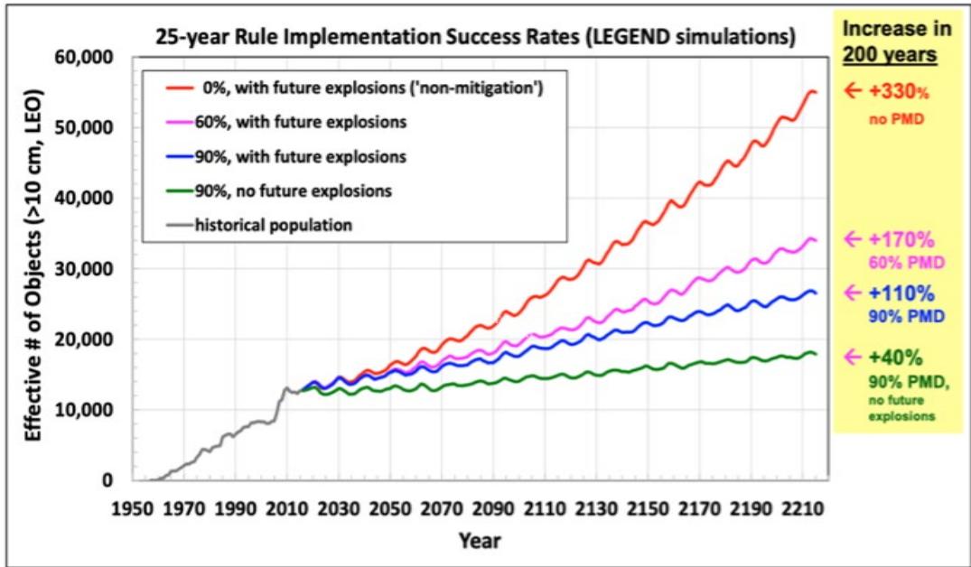#### Data description This paper's quantitative analysis incorporates observational, simulated, and derived data based on literature, experts' judgments, and publications by government agencies. Critical statistical inference uses data included in the studies published by the National Aeronautics and Space Administration Orbital Debris Program Office (NASA ODPO), debris collection risks, and the effective number of objects cited in NASA orbital debris quarterly newsletters (NASA ODQN), space economy data in Space Foundation reports, and space launch vehicle licensing data provided by the U.S. Federal Aviation Administration's Office of Commercial Space Transportation (FAA/AST) has made observational data available in the public domain, including the data used in NASA ODPO's orbital debris studies (NASA OIG, 2021) [1], J.-C. Liou (2011) [2], and other literature (N. Adilov et al. 2015) [3]. Unobservable data due to proprietary business practices are derived and simulated based on experts' judgment and data presented in literature. Employing variables for simulations, this study assigns statistical parameters to data points as they are probabilistic inputs. When constructing data sets pertaining to the cumulative number of catastrophic collisions for analyses and statistical inferences, this study applies collision scenarios in a low-case, a mid-case, and a high-case, as illustrated in (NASA's ODPO, 22-3, 2018, p. 5, Figure 5). The baseline for simulating the costs of orbital debris and the costs of mitigation in its studies matches findings and simulation results presented by NASA's ODPO, including the effective number of object projections, the 25-year rule implementation success rates (LEGEND simulations, Figure 4) [13], the cumulative number of catastrophic collision projections, the accidental explosion probabilities of large constellations, and catastrophic collision numbers. For spacecraft replacement simulation, table 3 aligns data with NASA ODPO's orbital debris studies for the data postulating collision probabilities of 0.01, 0.001, 0.0001, and 0 corresponding with active projects increasing by $1160\%$, $590\%$, $530\%$, and $5240\%$; PMD at $90\%$, $95\%$, 99%, and 99.9%; and a 100% success rate corresponding with catastrophic collision numbers of 582, 158, 40, 32, and 27 respectively (NASA's ODQN, 22-3, 2018, Figures 7 and 8, pp. 6 and 7)[5]. This study constructs unobservable data points for mitigation unit cost by using U.S. information at the current rate of post-mission disposal based on space experts' judgment. In the monetization procedures, all monetary values are expressed in 2019 dollars as undiscounted values, and then present values are derived at a $3\%$ discount rate. Concerning simulation data, this paper uses Monte Carlo simulations with the statistics software application Palisade @Risks. #### Method details #### Models The following models are designed for break-even analysis. The model determines a break-even point where the cost stream of orbital debris equals the cost stream of space preservation. $$ E q u a t i o n (1): f a (n, p, t) = (A 1 + R 1) + (A 2 + R 2) + (A 3 + R 3) + \dots + (A t + R t) + \varepsilon t., w h e r e t = y e a r, - - E q. (1) $$ $$ E q u a t i o n (2): f b (n, p, t) = (M 1 + C 1) + (M 1 + C 1) + (M 1 + C 1) + + (M t + C t) + \varepsilon t., w h e r e t = y e a r, - - E q. (2) $$ Where Eq. (1) represents the cost of orbital debris and Eq. (2) represents the cost of space preservation. Both streams are functions of debris number $(n)$, collision probability $(\rho)$, and time $(t)$. Furthermore, in 1000 simulation runs, the mean of the variance residuals $(\varepsilon_{t})$ is assumed to be zero. The starting time is 1990, and the ending time is 2150. All negative values are transformed into positive values. Monte Carlo simulation is a process that assigns a probability distribution to each of the inputs. In Eq. (1), the inputs are the share of the space economy, the growth rate of the global space economy, and the cumulative number of spacecraft replacements, assuming the price of replacement is a constant. The inputs for Eq. (2) are the affected number of mitigation and mitigation cost per launch. Running simulations, a computer program calculates the output of the model a thousand times. Based on the defined input probability distributions, the computer program generates a different value for each input parameter on each trial. Statistics on the output variables of interest are calculated at the end of the simulation. The term "space economy" is a novel concept in modern economics, with numerous interpretations. This paper employs the phrase "the space economy, which is the full range of activities and the use of resources that create and provide value and benefits to human beings while exploring, understanding, managing, and utilizing space. Hence, it includes all public and private actors involved in developing, providing, and using space-related products and services, ranging from research and development, the manufacture and use of space infrastructure (ground stations, launch vehicles, and satellites), to space-enabled applications (navigation equipment, satellite phones, meteorological services, etc.), and the scientific knowledge generated by such activities." (OECD 2012) [4]. ## I. THE MONETIZATION OF THE COSTS OF SPACE DEBRIS ### a) The model for estimating the cost of space debris According to Eq. (1), the costs of space debris are comprised of two components: awareness costs $(A_{t})$ and mission replacement costs $(R_{t})$. In Eq. (1), the awareness cost $(A_{t})$ can be drilled down to be the global space revenue as an alpha $(\alpha)$ share of the global space economy $(G_{a})$ multiplied by a cost attribute rate $(\gamma)$; mission replacement costs $(R_{t})$ can be expressed by an expected number of catastrophic collisions $(N_{a})$ multiplied by the replacement cost per spacecraft $(P_{a})$. As a result, costs of space debris Eq. (1) = awareness cost $(A_{t}) +$ mission replacement cost $(R_{t}) = \alpha \gamma G_{a}(t) + N_{a} P_{a}(t) + \varepsilon_{t}$. ### b) Variables In the following, there are discussions of methods for estimating each of the parameters and variables related to Eq. (1). historical time series from 1990 to 2019 and an extrapolation of the space economy from 2020 to 2150, a 160-year analysis period. This study goes through two stages. The first stage forecasts the global space economy from 2020 to 2049 based on the past 20 years of historical observations; the second stage simulates the space economy for the next 100 years by employing Monte Carlo 1000-runs. The global space economy forecast is based on time series data between 2005 and 2019 from Space Foundation Reports [6]. The forecast model makes use of an exponential smoothing algorithm, which works best with Excel's forecast functions. The forecasted series output in Figure 2 is an example generated with target date, historical values, and timeline inputs. Table 1 displays the observations and the growth rates for the space economy Figure 2 depicts the forecasting output for the period between 2005 and 2049. This paper compared this study to those conducted by other entities as corroboration. Table 1 shows that the average growth rate in the 10-year period from 2005 to 2020 was around $7\%$, except in 2015, when the space economy experienced negative growth. This $955 billion projection for the global space economy in Figure 2 is conservative when compared to bank projections for the year 2040 ranging from $926 billion to $3 trillion (Table 2). The true outlook for a specific economic sector beyond 30 years, to a distant future in 2150, is probabilistic in a simulation process. With a conservative outlook, a long-term growth rate of around $7\%$ for any economic sector of the global economy is deemed less likely. For this reason, this study undertakes Monte Carlo simulation approaches. In the process of relating the space revenue to the global space economy, this study assigns probabilities to inputs with minimum, mean, and maximum values matching the output of the forecasted series in Figure 2; additionally, it assigns probabilities of $50\%$, $75\%$, and $90\%$ to a $7\%$ average growth rate to simulate the space economy time series. (3) Cost attribution rate $(\gamma)$: This rate means a percentage of space revenue is attributable to orbital debris awareness costs. This paper quantifies the cost attribution rate $(\gamma)$ in the range of $1\%$ to $5\%$ based on the corroboration of various historical data points, experts' opinions, and the literature (ESA, "The Cost of Space Debris," July 5, 2020) [10]. (4) Variable $N_{a}(t)$: This represents the expected number of catastrophic collisions. The simulation of cumulative catastrophic collision numbers is a probabilistic process. This analysis uses cumulative collision numbers between 30 and 270 around the year 2150, aligning with the projections reported by NASA ODPO (Figures 3 and 4). There are two sources of explosions: background orbital debris explosions (BG_exp) and large constellation orbital debris explosions (LC_exp). This range matches the assumptions, defined as a range between the upper bound at which GB_exp with post-mission disposal at a 90 percent rate (BG_exp_90% PMD) and LC_exp_90% PMD, and the lower bound of BG_exp_90% PMD and LC_exp_99% PMD for 50 years of replenishment and 6,700 spacecraft (ODQN 22-3) (Figure 5) [6]. (5) Variable \(P_{a}(t)\): It is the value of each replacement, which is set between \\(50 million and \\)96 million for 500 Monte Carlo runs to construct a time series of mission replacement costs \((R_{t})\). The initial value is \\(96 million, which is decreasing over time. c) Estimate the costs of space debris In a nutshell, the following steps are taken in this paper to monetize the costs of space debris. - (a) Simulate the global space economy time series $G_{a}(t)$ by setting statistical weights at $50\%$, $75\%$, and $90\%$ for the space economy based on the average $7\%$ growth rate of the past 15 years. - (b) Derive the space revenue time series by multiplying $G_{a}(t)$ by the parameter alpha ( $\alpha$ ) at a 74% rate. - (c) Simulate the debris awareness costs of three scenarios by applying the cost attribute rate $(\gamma)$ ranging from $1\%$ to $5\%$ to the space revenue. - (d) Simulate the space mission replacement cost in three scenarios. Multiplying lower-case (50%), mid-case (75%), and higher-case (100%) for cumulative catastrophic collision numbers by a unit replacement value of $96 million to simulate the values of mission-spacecraft losses. - (e) Calculate the present value of the costs of space debris at a $3\%$ discount rate and substitute simulation output into equation (1). ### d) Assumptions and Data The models rest on the assumptions used in NASA's ODPO study for collision probabilities, area-to-mass ratio, and active object predictions [5]. The cost of orbital debris will continue to rise as orbital debris is allowed to proliferate. The projection of long-run space economy growth and space revenue are primary inputs into the analyses used to support long-term predictions of orbital debris costs. Uncertainties are inherent in the predictions from numerical simulation models for space economy and the cost attribution rate. It is appropriate that uncertainties are factored into the cost simulations by setting a range of probabilities to a current observed average growth rate and the experts selected cost contribution rate $(\alpha = 5\%)$. Since the 2020 ESA research paper predicts the cost contribution rate $(\alpha)$ to be $5\%$, this paper goes above and beyond to confirm the rate with observations from the space community [10]. These observations are discussed in the original paper [14]. Being cautious and not overstating the long-term cost of orbital debris, the paper applies a range of the cost contribution rate $(\alpha)$ range of $1\%$ to $5\%$ to the forecasted space revenue. ## II. THE MONETIZATION OF SPACE PRESERVATION The costs of post-mission disposal (PMD) and active debris removal determine the monetarization of space preservation measures (ADR). PMD options include uncontrolled atmospheric disposal, controlled disposal, direct retrieval, heliocentric Earth-escape disposal, and maneuvering post-mission objects to disposal orbits. ADR, or direct retrieval disposal, is a method of orbital debris disposal that involves removing human-made objects from protected Earth orbits beyond the mitigation guidelines currently adopted by the international space community. ### a) The model of estimating the costs of space preservation Eq. (2) shows that the costs of space preservation include mitigation costs $(\mathsf{M}_{\mathsf{t}})$ and remediation costs $(C_{t})$. This equation can be further deconstructed by multiplying the PMD success rate $(\beta)$ by the mitigation unit cost $(C_{b})$ and the affected launch numbers prediction $(N_{b})$ to get the mitigation cost $(M_{t})$, plus the expected number of active removals of defunct spacecraft $(N_{c})$ multiplied by the present value per launch $(P_{c})$ to get the remediation cost $(C_{t})$, plus the mean of the variance residuals $(\varepsilon_{t})$. As a result, costs of space preservation Eq. (2) = mitigation costs $(M_{t}) +$ remediation costs $(C_{1}) = \beta C_{b}N_{b}(t) + N_{c}P_{c}(t) + \varepsilon_{t}$. ### b) Variables In the following, there are discussions of methods for estimating parameters and variables related to Eq. (2). space preservation in this analysis conforms to a $20\%$ to $30\%$ rate of PMD with no ADR occurring. As a result, the initial value of parameter $(\beta)$ is set for an initial success rate of $20\%$ for PMD, which is assumed to increase linearly over time to a rate of $90\%$ in 2049. (2) Variable $C_b(t)$: It is a mitigation unit cost that is attributable to additional propellant, debris avoidance R&D, software and hardware testing, and engineers' time. Because global mitigation cost data are not available, this analysis extrapolates global mitigation costs from U.S. data, which are based on experts' judgment and knowledge. This study establishes experts' opinions on mitigation unit cost for Monte Carlo simulation runs ranging from a minimum to a maximum value. The simulation runs yield a mean of experts' judgments of about $4\%$ of a single medium-sized vehicle's launch cost. (3) Variable $N_{b}(t)$: This is the global affected number of launch vehicles subject to PMD at a 90% success rate. This paper presumes that future mitigation costs will be primarily attributed to commercial spacecraft launch activities. As a result, this study uses numbers of commercial launches excluding the suborbital as a reliable predictor of affected launches subject to mitigation. Furthermore, because the affected launch number is a subset of global total launches, this study estimates a multiplier parameter (X) based on U.S. data to infer the global mitigation $N_{b}(t)$. Table 4 data shows that the global space launch total is 4.21 times the U.S.-licensed space launches based on historical world launch data between 2011 and 2020 (Bureau of Transportation Statistics, bts.gov) and U.S. commercial spacecraft launch license data (FAA/AST) [10]. To corroborate the finding, Figure 3 depicts the derivation of the multiplier parameter (X) using the statistics software tool (Palisade @Risks) to infer the multiplier (X) parameter to be 4.28, which scales the U.S. effective number of space objects to the global total over a ten-year period. Using Monte Carlo simulation, the distribution shape appears close to a normal distribution in the range of a minimum of 2.9 to a maximum of 6.21, and around the mean of 4.28 (the multiplier parameter X) from Monte Carlo 500 runs at a 90% confidence level within 3.3 and 5.4. The statistics comparison table adjacent to the distribution figure uses two colors, red and blue, for the purpose of comparison between Monte Carlo simulation and PERT distribution. In Figure 3, the red area represents the inference value area covered by a 90% confidence level using Monte Carlo simulation, while the blue area covered by the PERT distribution with the minimum (2.85) and maximum (4.15) values shown. (4) Variable $N_{c}$: This is the expected number of active removals of defunct spacecraft from LEO and GEO. It is assumed to be zero in 2020 and five per year by 2049. (5) Variable $P_{\mathrm{c}}$: This is the present value of the single launch cost for the remediation. This paper assumes an undiscounted value of the LEO launch cost of approximately $96 million for each ADR mission. Over time, its present value per launch decreases. ### c) Estimate the costs of space preservation In sum, estimating the costs of space preservation involves the following steps. - (a) Estimate U.S. unit costs of PMD mitigation by averaging the costs of PMD options such as atmospheric disposal and maneuvering upper stages into storage orbit. The costs of each mitigation option are determined by the subject experts. - (b) Estimate Eq. (2) the multiplier parameter (X) by scaling the U.S. effective number of space objects to the global total over a 10-year period (the NASA ODQN between 2011 and 2020). - (c) Derive the world mitigation costs by multiplying the U.S. mitigation cost by the multiplier parameter (X), which is a parameter that scales US mitigation cost estimates to the global total. - (d) Simulate the costs of future active debris removal. The global remediation costs are gradually phased in and are expected to reach the maximum ADR per year in 2049. Presumably, five active debris removals (ADR) will cost approximately $96 million. The costs of remediation are fully accounted for when 5 ADR is in practice. The cost per ADR decreases over time. - (e) Estimate the present value of the costs of space preservation using a $3\%$ discount rate and plug simulation results into the equation (2). 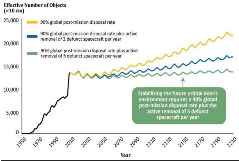### d) Assumptions and Data The models are based on the assumptions made in NASA ODPO's study [5]. In the study, its simulation graphics (Figure 6) illustrate conducting PMD at a $90\%$ rate and removing at least 5 defunct spacecraft per year to effectively stem the rising trend of the effective number of objects or the trend of orbital debris. The goal is reached when the preservation measures are fully implemented. The estimation of the preservation cost can be varied by the cost of forecasted PMD, the cost per ADR, and the number of ADR in a time series. The cost of forecasted PMD measures incorporates uncertainty in the predictions from the model for space launch forecasting and space vehicle launch cost. The data used for global space vehicle launch forecasting are based on US launch forecasting data. While a reliable global mitigation cost is not available, the rationale for using the U.S. launch forecasting data is that the U.S. data has the most available data points, and the U.S. currently accounts for the lion's share of the global space launches. Technically, using the X multiplier, which is a parameter that scales the U.S. mitigation cost estimates to the global total, is appropriate to bridge the data gap. ## III. BREAK-EVEN ANALYSIS Using Eq. (1) and Monte Carlo simulations, the best-fit model is an exponentially upward trend depicting the cost of orbital debris. As shown in Figure 7, the yellow curve (l) represents the cost of orbital debris, which stands for the cost stream of orbital debris proliferation. Under the status quo, post-mission upper stages are minimally mitigated at a $25\%$ (the midpoint of $20\%-30\%$ ) rate of PMD. Applying Eq. (2), the green curve II represents the cost of preservation, including mitigation and remediation. The yellow curve (I) is viewed as an exponential trendline, illustrating a rise in value at an increasing rate. The green curve (II), representing the cost of space preservation, is shown as a logarithmic trendline, which quickly increases then levels off. Although both trendlines are rising, they are converging and then crossing at their parity values at a break-even point. The third curve (brown, curve III) embodies the cost of orbital debris and the cost of space preservation. The presumption is that the impacts of orbital debris will be stabilized when the active removal of five defunct spacecraft per year and PMD with a $90\%$ success rate are fully phased in at some point on the time horizon. When the total amount of orbital debris is stabilized, its cost will be leveled because its accumulation rate is approaching a minimum. As a result, the third curve can also be viewed as the realization of the cost of orbital debris retention plus the costs of recurring preservation. The third curve is the sum of the values represented by curves I and II before the break-even point (BEP). Following the BEP, curve III is the sum of sunk or unsalvageable costs embodied in future spacecraft operations caused by orbital debris plus the cost of space preservation. Figure 7 depicts how debris mediation and remediation measures can slow or even halt the growth of orbital debris costs. As a result, when sufficient preservation measures are fully implemented, presumably in 2049 according to the NASA OIG's report 2021 [1], the cost of debris awareness and replacement will have passed its peak and will begin to fall. As a result, at the BEP, the brown curve (III) intersects the yellow curve (I). When the BEP is passed to the right, the variable cost includes the incremental cost of the mitigation and remediation over and above the sunk cost. Overall debris costs are decreasing from the BEP due to avoiding a future rise in the cost of space objects. Both the brown curve (III) and the green curve (II) are decreasing in part due to an economic discount mechanism that uses a $3\%$ discounted rate to calculate discounted future value. Figure 7 shows that the cost of space debris (the yellow curve) passing BEP from the left is greater than the brown curve (III); the difference between the two cost curves represents the cost savings. The brown curve (III) represents the reduced cost of orbital debris and space preservation. It means that the cost of orbital debris would be at an elevated level, as shown by the yellow curve (I), without further measures of space preservation. The accumulative cost savings over the next 100 years will equal the triangle area closest to the BEP, below the yellow curve (I), and above the brown curve (III). The cost savings will be enormous—approximately $2 trillion. ## IV. SENSITIVITY ANALYSIS Policy factors used in this sensitive analysis are considered, as shown by Figure 8. They are the discount rate for present value, the number of active accumulations of objects, the mass of active objects, the time factor for phasing in the preservation measures, and sustained objects in protected orbits. This paper demonstrates that the BEP movement resulted from changes in these independent variables. The total amount of orbital debris is equal to the number of active objects (n) multiplied by the total object mass (m) multiplied by the object-year in orbit (t). The third cost curve (III), which is dependent on the three variables multiplied by the cost per unit (i.e., n * m * t * $), influences the expected outcomes of BEP. When variables change, this model explains BEP movement. The number of active space objects is assumed to be the same as the number of space vehicles launched. The upper stages of post-mission spacecraft contribute the most mass to orbital debris. When this variable is applied to the US share of total commercial launches being surpassed by shares from other countries such as China, India, Korea, Brazil, Saudi Arabia, and so on, the model predicts that debris mitigation costs will rise, pushing BEP to the right. The time factor refers to the phases of implementation of the anticipated preservation measures. The preservation measures are the PMD at a $90\%$ discount rate and the 5-ADR, both of which affect BEP results. According to this model, delaying active debris removal in practice would result in a significant reduction in cost savings because delayed remediation would put the break-even point (BEP) at a higher cost level, thus pushing the BEP further into the future. As measured by the above model $(n * m * t)$, a higher BEP level is the consequence of rising cumulative debris. Another scenario in which the timing factor pushes BEP to the right assumes that the scheduled 5-ADR rate falls to 2 ADR per year. Because the spacefaring community in this scenario would have to spend more on awareness costs, both mitigation and remediation costs would rise in the future. As a result, insufficient ADR measures in timing contribute to raising the cost level predicted by the breakeven point (BEP). The cost of space debris is affected by the projected effective number of space objects associated with future launch activities as well as the timeline for implementing effective preservation measures. BEP movements and changes in the cost of realized orbital debris are explained by sensitivity analyses. A sensitivity analysis was conducted by considering the increase in active debris removal (ADR) to be greater than five used space stages. A number higher than 5 ADR would add additional remediation costs for space preservation. But that might be necessary to counter either used space stages rising faster than what observations suggest or remediation compliance being delayed to a distant future. However, declining ADR costs over time could offset the costs incurred with higher ADR numbers. Additional measures can be paid for by contracting for future remediation costs and expanding the long-term cost savings. All of that is reflected by the triangle area on the right side of the BEP. When the discount rate for assessing present value goes up, it makes today's dollar more valuable than a present value discounted by a lower discount rate, which should be around the nominal long-term growth rate of the space industry. As this study has a long analytical period of over 100 years, a discount rate greater than $3\%$ will overly discount future value. The present values of the costs in this break-even analysis use a $3\%$ discount rate. The federal Office of Management and Budget (OMB) directs all U.S. federal agencies to use $3\%$ for long-term analysis in federal regulatory analyses. Therefore, using a $3\%$ discount rate greater than a long-run growth rate to calculate the present value of the cost is appropriate. ## V. CONCLUSION The break-even analysis is an important decision-making tool that informs policymakers about space preservation choices and timing urgency. This analysis has made many simplifications because historical data are difficult to get. This paper strictly relies on NASA's studies regarding the accumulative number of space objects, orbital debris mass, collision probability, and space preservation measures. Since some of these assumptions are implicit, this paper takes an approximation of these observations without looking at detailed study data. As the cost of orbital debris is based on space activity forecasting, using U.S. observations can be problematic as the global space competition changes the reality quickly. The timing assumptions are critical for constructing the figures of the break-even analysis. In the end, this analysis extends the time frame into the distant future and thus limits its applicability. Using multi-decade timescales, a wide range of probabilities for the future's monetary value should be considered. ### APPENDIX Table 1: Global Space Economy between 2005 and 2020 (Space Foundation Reports) [6] <table><tr><td>Year</td><td>Global Space Economy* ($B)</td><td>Historical Growth Rate %</td></tr><tr><td>2005</td><td>175</td><td></td></tr><tr><td>2006</td><td>195.3</td><td>12%</td></tr><tr><td>2007</td><td>215.6</td><td>10%</td></tr><tr><td>2008</td><td>235.9</td><td>9%</td></tr><tr><td>2009</td><td>256.2</td><td>9%</td></tr><tr><td>2010</td><td>276.5</td><td>8%</td></tr><tr><td>2011</td><td>289.8</td><td>5%</td></tr><tr><td>2012</td><td>304.3</td><td>5%</td></tr><tr><td>2013</td><td>314.2</td><td>3%</td></tr><tr><td>2014</td><td>330</td><td>5%</td></tr><tr><td>2015</td><td>323</td><td>-2%</td></tr><tr><td>2016</td><td>329</td><td>2%</td></tr><tr><td>2017</td><td>385</td><td>17%</td></tr><tr><td>2018</td><td>414.5</td><td>8%</td></tr><tr><td>2019</td><td>423.8</td><td>2%</td></tr><tr><td>2020</td><td>447</td><td>5%</td></tr></table> Table 2: 2040 Projections of the Size and Composition of the Space Economy <table><tr><td>Space Economy Projections ($B)</td><td>2016</td><td>2040</td><td>Compound Annual Rate of Growth</td></tr><tr><td>UBS</td><td>$340</td><td>$926</td><td>4.3%</td></tr><tr><td>Morgan Stanley</td><td>$339</td><td>$1100</td><td>4.9%</td></tr><tr><td>U.S. Chamber of Commerce</td><td>$383.5</td><td>$1500</td><td>6.0%</td></tr><tr><td>Bank of America</td><td>$339</td><td>$2700</td><td>9.0%</td></tr><tr><td>Goldman Sachs</td><td>$340</td><td>$3000</td><td>9.5%</td></tr><tr><td>Average compound Annual Rate of Growth</td><td></td><td></td><td>6.7%</td></tr></table> Table 3: Collision probabilities and catastrophic collision numbers used by NASA's ODPO <table><tr><td colspan="4">Projected for Year 2215</td></tr><tr><td>Collision Probability over 5-years mission</td><td>Active Projects Increase by%</td><td>PMD%</td><td>Catastrophic Collisions Number</td></tr><tr><td>0.01</td><td>1160%</td><td>90.0%</td><td>582</td></tr><tr><td>0.001</td><td>590%</td><td>95.0%</td><td>158</td></tr><tr><td>0.0001</td><td>530%</td><td>99.0%</td><td>40</td></tr><tr><td>0</td><td>524%</td><td>99.9%</td><td>32</td></tr><tr><td>No Constellation</td><td>0</td><td>100%</td><td>27</td></tr></table>    Table 4: Successful space vehicle launch scale of the US vs. the world <table><tr><td>Successful Space Launch</td><td>The World Total</td><td>The US Total</td><td>The World Multiplier</td></tr><tr><td>2011</td><td>78</td><td>17</td><td>4.59</td></tr><tr><td>2012</td><td>73</td><td>12</td><td>6.03</td></tr><tr><td>2013</td><td>78</td><td>20</td><td>3.90</td></tr><tr><td>2014</td><td>88</td><td>20</td><td>4.40</td></tr><tr><td>2015</td><td>81</td><td>14</td><td>5.79</td></tr><tr><td>2016</td><td>82</td><td>17</td><td>4.82</td></tr><tr><td>2017</td><td>84</td><td>22</td><td>3.82</td></tr><tr><td>2018</td><td>111</td><td>35</td><td>3.17</td></tr><tr><td>2019</td><td>97</td><td>32</td><td>3.03</td></tr><tr><td>2020</td><td>110</td><td>39</td><td>2.89</td></tr><tr><td>Mean</td><td></td><td></td><td>4.21</td></tr></table>  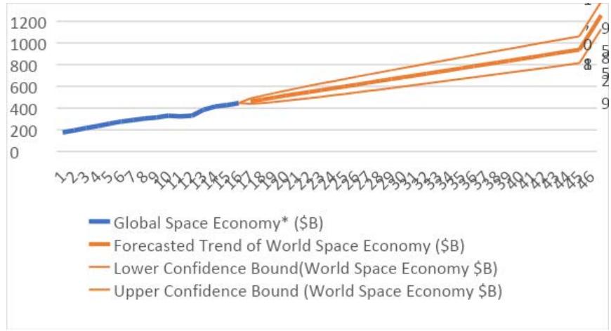Figure 2: Forecasting of the global space economy  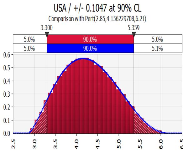Figure 3: Relationship between the size of the US space sector and the size of the remaining global Space sector <table><tr><td></td><td>USA / +/- 0.1047 at 90%</td><td>Pert (2.85,4.1562297)</td></tr><tr><td>Cell</td><td>Mitigation Co..</td><td>Mitigation Co..</td></tr><tr><td>Minimum</td><td>2.8998</td><td>2.8500</td></tr><tr><td>Maximum</td><td>6.0274</td><td>6.2100</td></tr><tr><td>Mean</td><td>4.2808</td><td>4.2808</td></tr><tr><td>90% CI</td><td>± 0.0327</td><td></td></tr><tr><td>Mode</td><td>4.1372</td><td>4.1562</td></tr><tr><td>Median</td><td>4.2512</td><td>4.2514</td></tr><tr><td>Std Dev</td><td>0.6284</td><td>0.6280</td></tr><tr><td>Skewness</td><td>0.1988</td><td>0.1984</td></tr><tr><td>Kurtosis</td><td>2.3916</td><td>2.3858</td></tr></table>  (Source: NASA's ODPO, Orbital Debris Quarterly News 24-1 February 2020, p5) [5] Figure 4: Projections based on the 25-year rule compliance levels and accidental explosions. Projection results are based on averages of 100 Monte Carlo simulations each. 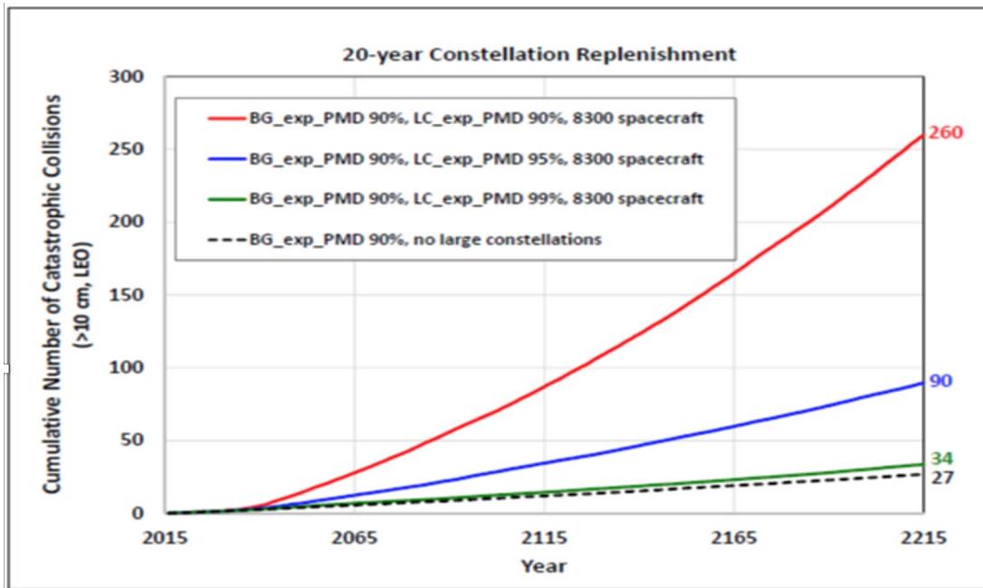 Figure 5: Cumulative collision numbers between 30 and 150 in 2150. Source: NASA ODPO, Orbital Debris Quarterly News 22-3 September 2018, p5  Source: NASA OIG depiction of ODPO information 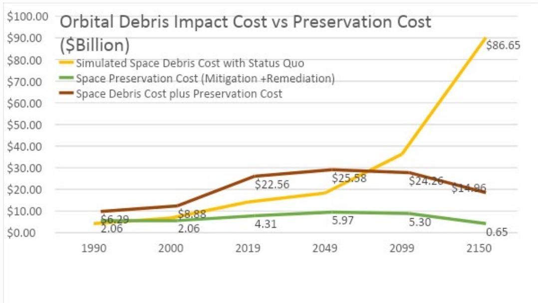 Figure 6: Global PMD at a $90\%$ rate plus ADR of 5 defunct spacecraft per year is needed to stabilize LEO's Orbital Debris Environment [1] Figure 7: The cost stream of extending orbital debris proliferation (curve I) crosses the cost stream of space preservation (curve III). The point of intersection is the break-even point (BEP). 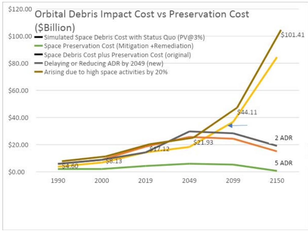 Figure 8: An example of sensitivity analysis. #### ACKNOWLEDGEMENTS The author is very grateful to Dr. Peter Ivory for his enlightening suggestions and important inputs. The author is also very grateful to anonymous reviewers and referees for providing valuable input to this article. Their suggestions and comments were essential in improving the clarity and quality of the paper. Declaration of interests The author declares that he has no known competing financial interests or personal relationships that could have appeared to influence the work reported in this paper.

Generating HTML Viewer...

References

10 Cites in Article
J.-C Liou Unknown Title.
Nodir Adilov,Peter Alexander,Brendan Cunningham (2015). An Economic Analysis of Earth Orbit Pollution.
Oecd (2012). OECD Handbook on Measuring the Space Economy.
J Beusch,I Kupiec (2018). NASA debris environment characterization with the Haystack radar.
Esa (2020). The Cost of Space Debris.
John Honeycutt,Chris Cianciola,John Blevins (2021). NASA's Space Launch System Begins Integration in Preparation for Launch.
S Licensed,Launches (2020). Unknown Title.
Paula Krisko (2003). NASA Long-Term Orbital Debris Modeling Comparison: LEGEND and EVOLVE.
Martin Zhu (2022). A break-even analysis of orbital debris and space preservation through monetization.
Colvin (2023). Cost and Benefit Analysis of Orbital Debris Remediation.
No ethics committee approval was required for this article type.
Data Availability
Not applicable for this article.
How to Cite This Article
Martin K. Zhu. 2026. \u201cMethod of a Break-Even Analysis of Orbital Debris Mitigation and Remediation Costs\u201d. Global Journal of Research in Engineering - J: General Engineering GJRE-J Volume 23 (GJRE Volume 23 Issue J2).
Explore published articles in an immersive Augmented Reality environment. Our platform converts research papers into interactive 3D books, allowing readers to view and interact with content using AR and VR compatible devices.
Your published article is automatically converted into a realistic 3D book. Flip through pages and read research papers in a more engaging and interactive format.
Our website is actively being updated, and changes may occur frequently. Please clear your browser cache if needed. For feedback or error reporting, please email [email protected]
Thank you for connecting with us. We will respond to you shortly.