I. INTRODUCTION

To gain insight for solving fluid mechanics' domain consisting of vivid aerodynamic or hydrodynamic problems, there are numerous ways, such as:

Flight Experiments, flying scale models, Rocket Sleds and Flights, Drop Tests, Water Tunnels as well as Water Tables, Whirling Arm Apparatus tests, Shock tubes, road tests, ballistic ranges and so many other techniques leading to an almost interminable list, where each test/device has its own domain of supremacy and none of them could be deemed as the "best" [45].

Amongst the above, the highly preferred device being Wind Tunnel Testing which could be subsonic, near sonic, transonic, supersonic or even hypersonic.

Wind tunnels are huge channels with airflow through them that have been used to simulate the interaction of air with an object that is flying through the air or advancing along the ground. Wind tunnels are used by researchers to gain a better understanding of how an aeroplane will fly. Wind tunnels are used by NASA to test scale models as well as replicas of vehicles and spacecraft. Some wind tunnels are large enough to fit full-size vehicles within themselves. The wind tunnel creates an illusion of flight by moving air around an object.

Large strong fans blow air through the tube most or all of the time. The object being inspected is securely retained within the tunnel, ensuring that it remains stationary and unperturbed. An aerodynamic structural member, such as a cylinder or an airfoil, an individual element, a small type of vehicle, or maybe even a full-sized waggon may be used as the object. The air moving around the fixed object simulates what would happen if the object were in motion. The motion of air can be scrutinised in a multitude of settings; for example, smoke or dye can be introduced in the air and observed as it moves around an object. To illustrate how the air moves around the object, colorful threads may also be attached to it.

The first wind tunnels were created near the end of the nineteenth century, during the early days of aeronautic research, when many people tried to build prolific bulkier, studier, and heavy-than-air flying machines. The wind tunnel was conceived as a way of reversing the normal paradigm: instead of the air remaining still while an object moves through it at high speed, the same effect could be achieved if the object remained stationary while the air moved past it at high speed. In this regard, a stationary researcher might study the flying object in flight and measure the aerodynamic forces acting on it.

The innovation of wind tunnels aligned with the development of the aircraft. During WWII, huge wind tunnels were constructed. During the Cold War, wind tunnel testing was deemed essential in the production of supersonic military aviation and ballistic missiles.

Thus, Wind tunnels are used to evaluate the subjects of aerodynamic research because they are capable of simulating actual airflow conditions through the test section. Despite their significance, however, wind tunnels are constrained by their expense, size, and inadequate knowledge of their design. The demand for wind tunnel tests has diminished, thanks to recent advances in computational fluid dynamics (CFD) modeling on high-speed computer technology.[8] However, The requirement for wind tunnels to elucidate intricate aerodynamics snags is still needed today. [1]

II. BACKGROUND

a) Different Research and Aerodynamic Study Methodologies

Theoretical/Analytical, computational, and experimental/practical approaches are all commonly used to solve aerodynamic engineering problems, each with its own set of protocols, range benefits and drawbacks. [45][46][55].

i. Theoretical/Analytical

They are confined to conjecture and speculation and are involved with the theory of a study or field of research.

Theoretical strategies are analytical approaches to solving fluid dynamics' governing equations. Analytical processes have the distinct advantage of producing closed form solutions. The formulae derived from an analytical approach may provide a lot of information about how the system will behave under various circumstances. Sadly, except in cases where the governing equations are linear or can be estimated as such, analytical solutions are indeed impossible to obtain or procure.

Considering only simple geometries, such as flow through an infinitely long pipe, is the only primary way to acquire linear governing equations. However, many interesting problems require complex geometries like cars or planes. Theoretical methods, but at the other hand, are essential for getting an understanding of the fundamental flow phenomena and acquiring insight for how given flow fields will interact. Theoretical methods are still significant in the confirmation of computational methodologies. Since computational solutions are approximations, evaluating the accuracy of computational algorithms on problems with analytical solutions is beneficial.

ii. Computational (CFD-Computational Fluid Dynamics)

The numerical approach to aeronautic design, also known as computational fluid dynamics, is the second approach. Any type of calculation that follows a well-defined model and covers both arithmetical and non-arithmetical steps is referred to as computation. It approximates the solutions to the governing equations of fluid mechanics using computational algorithms. The geometry for a given flow problem must be reproduced employing CAD. The flow domain must then be discretized into a grid/mesh, with initial and boundary conditions determined. The solution is assumed to be constant in each cell in several methods, and the governing equations are also discretized to model how the solution changes in each cell.

The simulation should begin after an algorithm has been determined. [46] Due to the relentless advancement in computing power and memory of computers, the field of CFD has seen explosive growth in the last fifty years. Because of the rapid advancement of computers in the 1960s and 1970s, some researchers predicted that computer simulations would ultimately be able to evaluate free flight scenarios more accurately than wind tunnels, and could even replace them entirely [56].

Unlike analytical techniques, CFD only requires a few assumptions to solve a problem and can also produce time resolved flow solutions for any problem. It is possible to perform viscous simulations on a complete plane in less than a day using a personal computer, depending on the methodologies adopted $[57]$. Furthermore, there are issues for which obtaining experimental data and it remains difficult or impossible. Taking measurements inside a jet engine, for example, is not always feasible. As a result, CFD has become an invaluable engineering tool for cutting the levels of experimental testing required in the aerodynamic construction process.

Despite its many perks, CFD seems to have some shortcomings that prevent it from entirely replacing wind tunnel testing. Truncation errors in floating point calculations are a complication in CFD, as in any field that depends on numerical methods. Because computers can only retain a finite number of digits in arithmetic operations, round-off errors can occur in CFD. The number of grid points determines the magnitude of the error. Discretization error is also introduced through CFD. When round-off error is removed, discretization error is defined as the difference between the partial differential equation solution and the discretized approximation to the differential equation solution $[55]$.

Furthermore, advances in computing power make a much easier remedy to increasingly complex problems. This is not always the case, though. That's because software parallelization is complicated. It's also worth noting that, while CFD can predict aerodynamic performance with increasing precision, engineers are often more obsessed with other characteristics like reliability, operability, and maintainability. CFD alone, for example, cannot predict whether an engine can revive cruise speed or how many flight hours can be attained before service is required. Turbulence modelling is another challenge associated with CFD.

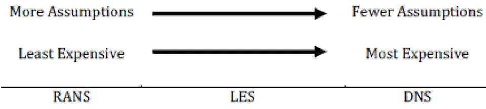
Direct Numerical Simulation (DNS) simulations are one method of modelling fluid flow. This approach does not approximate the governing equations and often involves orders of magnitude more mesh points than a computationally less expensive alternative like Reynolds- Averaged Navier-Stokes (RANS) [55] [56] [57]. RANS, on the other hand, is one of the most widely used CFD algorithms in engineering. It works by averaging the Navier-Stokes equations over time statistically. While RANS techniques can be used in cases of minor separation, they are often ineffective in cases of massive separation [57].

Large-eddy simulation (LES) is a different strategy to CFD. In the same way that RANS does, LES makes assumptions that lead to approximations of the Navier-Stokes equations. It filters the Navier-Stokes equations instead of averaging them, eliminating high wave-number components [59].

This method's computing cost and accuracy are comparable to RANS and DNS.

Despite these and other weaknesses, CFD has demonstrated to be an amazing resource in the aerodynamic design process, substantially reducing the number of design cycle iterations required.

iii. Experimental/Practical

This third method of achieving aerodynamic probabilities is experimental and involves or employs analysis or logical reasoning; it refers to a person, concept, project, or other entity that is more concerned with or applicable to practise than hypothesis and can be done or implemented.

Since the time of the Wright brothers, wind tunnel testing has been used as the foundation for the design of all current flying crafts. Even though the number of military aircraft initiatives has been declining since the 1950s, the number of wind tunnel test hours per program has been continuously growing [8]. This is due to the fact that as aeroplanes become more sophisticated, the amount of testing required to perfect a design grows. The amount of experimentally gained data for an aircraft programme has grown in recent years and will continue to do so in the future.

Wind tunnels, on the other hand, have their challenges. The cost of building and maintaining a wind tunnel, for example, varies depending on its size and characteristics, but it is seldom a low-cost undertaking. This is due to the fact that designing and building a wind tunnel will take years and numerous man-hours. Making precise models with correctly calibrated equipment is a daunting task that only adds to a wind tunnel's operating costs. The most difficult aspect of wind tunnel testing is accurately replicating flow parameters. This entails creating a model of the object of interest and replicating the desired Reynolds number at low speeds.

In addition, there are two main types of aerodynamic problems:

1. External aerodynamics, which refers to solid bodies immersed in flow, such as those found around wings or aerofoils.

b) All about Wind Tunnels

i. The Gist of Wind Tunnels

As stated earlier, the science of aerodynamics concentrates on studying the echt (real) impact or generation of airflow of various speeds on solid objects. An inseparable tool of testing-The wind tunnel, is used in educational research, to study/simulate/analyse the effects of air moving past solid objects, under various conditions, about complete aircraft or aircraft components, the forces acting on them and their interaction/ behaviour with the air flow. Experiments are used for commercial purposes, such as studying the aerodynamics of vehicles to enhance their stability and effectiveness, and also for educational purposes, such as understanding complex fluid flows and multiple model responses to an airstream. As a result, a wind tunnel is an important tool in both fluid mechanics and experimental aerodynamics. They come in a variety of shapes and sizes, spanning from 30cm to the dimensions of a passenger aircraft. [52, 19, 26, 43, 9, 5, 49, 53, 30, 44, and 23]

A well-designed wind tunnel could supply technical information for a large number of engineering applications such as external aerodynamics (flow over automobile, terrestrial and aerial vehicles) [43], civil engineering (estimation of pollution dispersion level near the building, investigation of wind-driven rain and building envelop, various aspects of wind loading on roofs and wind effects on towers and bridge. [52], flow over cable stayed bridges, high rise buildings, cable, electricity transmission towers etc.), sport activities (flow over cyclists, design of volley and basket balls, wind sails etc.), fundamental fluid dynamics (laminar and turbulent flow over simple and complex geometries) and an extensive frame of other options in industry and research centres at universities around the world, for a varied number of reasons such as testing of prototypes early in their design cycles, or to record a large amount of data.

It's a tube or tunnel with different cross sections in which man-made wind is blown at a controlled speed through a closed tubular passage, with the object under test mounted in the middle of the test compartment. Engineers and scientists place a model (made of steel or aluminium) of an aircraft, truck, or full-scale wind turbine in this section and investigate how air moves around it. They can get a pretty good idea of how a real-life-sized system with the same designs would respond by looking at how this smaller model interacts in the wind tunnel. [26] Aerodynamicists need to use the wind tunnel's controlled environment to measure flow conditions and forces on aircraft models as they are being developed. The ability to gather diagnostic data from models allows engineers to tweak designs for aerodynamic performance in a cost-effective and safe manner without having to construct countless fully functional prototypes.

Air is moved past the object by a strong fan system comprising of one or more fans; the fan must have straightening vanes to smooth the airflow. The test object is fitted with a delicate balance to measure the forces produced by airflow; alternatively, smoke or other substances may be injected into the airflow to make the flow lines around the object visible.[26]

The National Aeronautics and Space Administration (NASA), Boeing, Northrop Grumman, and every other company that manufactures aeroplanes and spacecraft use wind tunnels today. NASA's Ames Research Center in Moffet Field, California, has the most wind tunnels of any location on the planet, as well as the world's largest wind tunnel. [53] These facilities are costly to run, and computer modelling has taken over some of their functions. [26]

The flow visualisation provided by a wind tunnel is one of the most significant features. Sure, complex equations can be used to determine lift, drag, and efficiency. The visual aspect of a wind tunnel, as well as the controllable environment it offers, helps you to physically see what will happen in a variety of real-life scenarios. In the confines of a test lab, you can make an environment where you can see how an aircraft reacts when taking off, cruising, and landing. Then, using the same machine, you can see how air flows over a race car's body as it speeds around a track in order to maximise productivity. The versatility and tangibility of a wind tunnel is what makes it such an important part of aerodynamic research. [19, 10, 25, 47] As a result, wind tunnel testing of full/model-scale components is a commonly used method for guiding detailed design decisions in thermal-fluid systems and allowing basic fluid phenomena study. Many times, theoretical and/or computational methods are insufficient, either due to the problem's complexity or a lack of appropriate computational resources. [23] The majority of experimental data required in aerodynamics is produced in wind tunnels, and for these reasons, wind tunnel testing is often the most cost-effective method. [10]

ii. Principle

The wind tunnel was conceived as a way of reversing the normal paradigm: instead of the air remaining stationary while the vehicle or aircraft moved at high speeds through it, the same effect could be achieved if the vehicle or aircraft remained stationary while the air moved at high speeds past it. A stationary observer may study the vehicle or aircraft in action and measure the aerodynamic forces acting on the aircraft in this manner. [26, 49]

iii. Performance

As a result, WT is a device that can be used to explore the interaction of solid body flows in terms of [19]:

1. Physical flow phenomena such as laminar, turbulent, and separation flows, vortex, and shock waves must be monitored.

2. Obtaining aerodynamic data such as pressure, skin friction, lift, and dragas well as moments.

When compared to free flight experiments, the wind tunnel offers many advantages:

1. Specified flow conditions such as Mach number and incidence can be obtained and maintained much more easily in a wind tunnel.

2. In a wind tunnel, dangerous, uncontrollable flight conditions can be investigated safely.

3. Direct connection to ground-based facilities simplifies data acquisition and processing.

The primary drawback of using a wind tunnel is that it is rarely possible to accurately recreate full-scale motion. This is mostly due to the use of scaled models in order to reduce tunnel costs and energy consumption.

iii. Quick Facts

1. World's First Wind Tunnel

Frank H. Wenham (1824-1908), a Council Member of the Aeronautical Society of Great Britain, is generally credited with designing and operating the first wind tunnel in 1871. [60].

2. World's Largest Wind Tunnel

The largest wind tunnel in the world is at NASA's Ames Research Center. This subsonic tunnel, which can test planes with wing spans of up to 100 feet, is over 1,400 feet long and 180 feet high [63].

3. Oldest Wind Tunnel

NASA Langley 30-by-60-Foot Full-Scale Wind Tunnel, NASA's oldest operating wind tunnel until its closing in October 1995 [64].

4. Fastest Wind Tunnel (Deemed)

It has been revealed that China is set to build the world's fastest hypersonic wind tunnel that will be used to aid the development of spacecraft. "The 265-meter-long tunnel can be used to test hypersonic aircraft that can travel at speeds of up to Mach 25 (30,625kph), 25 times the speed of sound," Han Guilai, a Researcher from China's State Key Laboratory of High Temperature Gas Dynamics of the Chinese Academy of Sciences. [61][62].

c) Types of different Wind Tunnels

i. High-Reynolds-Number Wind Tunnels

It is often impractical to obtain full-scale Reynolds numbers in an experimental facility using a full-scale vehicle; however, there are ways to increase the Reynolds number using smaller tunnels and models. [45]

a. Pressurized Wind Tunnels

One of the oldest methods is to construct a pressurised tunnel. In fact, pressurised tunnels were used to conduct some of the first definitive research on Reynolds number effects. Examining the equation of state for a perfect gas and the equation for Reynolds number reveals the reason for pressurisation: increasing the pressure by a factor of 20 increases the density, and thus the Reynolds number, for a given size and speed by 20 times

Some fundamental issues concerning the construction and operation costs of pressurised tunnels must be considered. For pressurised tunnels, the cost of compressor equipment will increase, and for larger facilities, providing access to the model test area without decompressing the entire tunnel will increase construction complexity and cost. Pressurized facilities require more time to change the pressure condition and access the model, which reduces the facility's productivity and thus raises the cost to users.

b. Different Working Fluid

Changing the working fluid is a second option. The use of Freon 12 can increase the Mach number by a factor of 2.5 and the Reynolds number by a factor of 3.6 for a given power input. Many of the problems that have plagued a pressure tunnel will resurface, including initial cost, pump costs, gas costs, and a method for making the test section habitable for model, changes. The National Aeronautics and Space Administration (NASA) Langley's Transonic Dynamics Tunnel is an example of a tunnel that began using Freon 12 as the working fluid in 1960. [45]

c. Cryogenic

The use of a cryogenic tunnel is a third option. The National Transonic Facility (NW), which NASA built at its Langley Research Center in the beginning of 1971 [36], was the first of its kind. The same concept applies to a low-speed tunnel, even though this tunnel is designed for transonic experiments. The NTF tunnel combines the ability to operate at cryogenic temperatures with the ability to change pressure up to 9 atm, making it the world's largest piece of cryogenic research equipment in operation. The working fluid is nitrogen, and the gas is cooled by injecting liquid nitrogen upstream of the fan. This technique allows any pressure tunnel to operate over a wide range of dynamic pressures and Reynolds numbers at a constant temperature up to the tunnel's stagnation pressure limit. Alternatively, the tunnel can be run at constant dynamic pressure and the Reynolds number changed by changing the temperature. The range of Reynolds and Mach numbers in units is impressive. This type of facility is both costly to build and operate, but it does demonstrate what can be accomplished in a wind tunnel. The NTF's low productivity has kept it from being useful as a development facility due to the long times it takes to cycle and stabilise the temperature.

The European Transonic Facility in Cologne, Germany, is another high-Reynolds-number tunnel based on cryogenic operation. It is a joint venture between the United Kingdom, Germany, France, and the Netherlands. KKK (Kryo-Kanai K61n): This large cryogenic wind tunnel was built at DLR Cologne as a conversion of a traditional closed-circuit fan-driven atmospheric pressure tunnel.[36]

ii. Vertical Short Take-off and Landing V/STOL Wind Tunnels

Because of the large downwash angles generated by powered lift systems in the transition flight region, these tunnels require a much larger test section for a given size model. The transition region has low flight velocities, so tunnels with large test sections used for this purpose do not require high velocities, with the maximum being in the 6&100 mph range, compared to the 200-300 mph range for a conventional low-speed wind tunnel. The installed power requirement is reduced because power varies with the cube of velocity. In both the Boeing Helicopter Co. (test-section area 400 ft2) and the NASA Langley VERTICAL SHORT TAKEOFF AND LANDING (V/STOL) tunnels, this was the solution.

iii. Free-Flight Tunnels

Many "free-flight" tunnels were constructed in the 1930s. These open-return tunnels were designed to allow dimensionally and dynamically scaled models to be flown under gravity's influence. The air stream could be tilted to match the model's glide path. In these tunnels, the model's dynamic behaviour could be studied, and control surfaces could often be deflected by a trailing wire. Because the simulations in these tunnels are done at very low Reynolds numbers, extrapolating the results to much higher Reynolds number conditions should be done with caution.

iv. Spin Tunnels or Vertical Wind Tunnels

The tendency of some aircraft to spin after a stall, as well as the need to determine actions to recover from the spin, have long been a source of concern for aircraft designers. In a spin tunnel, the recovery from a spin is studied. In most cases, this is a vertical wind tunnel with air drawn upward by a propeller near the tunnel's top.

v. Stability Tunnels

In 1941, NASA Langley constructed a stability tunnel. There were two 6 ft. long interchangeable test sections in this tunnel. In one test segment, a series of spinning vanes formed a vortex in the airstream. The second test section was bent to mimic turning take-off. The tunnel was moved to Virginia Polytechnic Institute and State University in 1958, and it is still used as a general-purpose and special-purpose wind tunnel there today. Related findings can be achieved using oscillating model techniques or free-flight tests in traditional tunnels. [45]

vi. Propeller Tunnels

Propeller tunnels are identical to traditional tunnels, but they usually have an open test section and a round cross section. Stanford University designed one of the first propeller tunnels in 1917, with a 5.5-foot-diameter test section. In 1922, NASA Langley built a propeller tunnel with a 20-foot test area. Aside from propeller tests, this tunnel revealed the best position for engine nacelles relative to the wing and the configuration of radial engine cowls (NASA cowl) to minimise drag.

vii. Propulsion Tunnels

The simulation of both flight velocity and atmospheric pressure and temperature variations is required for experimental evaluation of aircraft engines, whether reciprocating or jet. The exhaust gases must be removed from a closed circuit tunnel or an open circuit tunnel must be used because the engine must be operated in the tunnel.

viii. Icing Tunnels

The NASA 6 X 9-ft Icing Research Tunnel, located near Cleveland, Ohio, is a low-speed closed return tunnel with a refrigeration device to lower the air temperature to -40°F and atomizers upstream of the test segment to produce water droplets that freeze. The tunnel's shell is tightly shielded, which helps to keep the tunnel cool. To keep the fan from freezing during model shifts, the facility requires that it be operated at idle rpm. Ice accumulation on aircraft is a significant safety concern for aircraft and helicopters flying at low to medium altitudes.

ix. Low-Turbulence Tunnels

In order to maximise the size of the settling chamber without raising the total circuit dimensions, these tunnels typically have a wide-angle diffuser just ahead of the settling chamber.

x. Two-Dimensional Tunnels

Airfoil portions are mainly evaluated in two-dimensional tunnels. They've been made in both open circuit and closed return configurations. Tall short test sections with height-to-width ratios of 2 or greater can be found in these tunnels.

xi. Smoke Tunnels

Smoke tunnels are mainly used to visualise flow. Since photos and video capture are the main types of data recording, these tunnels are usually non return. Smoke tunnels of two and three dimensions have been constructed. While many other products have been used as smoke sources, current usage seems to favour vaporised light oils, kerosene, or propylene glycol. To achieve smooth laminar flow, smoke tunnels used for testing rather than demonstration purposes often have very high contraction ratios (up to 24:1) and a large number of antiturbulence screens at the inlet. Smoke tunnels are typically slow, moving at 30-60 feet per second.

xii. Automobile Wind Tunnels

Experiments are conducted with miniature models or at full scale in larger tunnels to obtain aerodynamic parameters that influence vehicle performance, handling, engine cooling, brake cooling, and wind noise. Contrary to popular belief, building tunnels to house full-scale vehicles is both practical and general practise. Using moderate scale models, such as 0.25-0.4, and doing tests at full-scale Reynolds numbers are also beneficial.

Examples

Several car manufactures and race teams use the Lockheed low-speed wind tunnel in Marietta, Georgia, as well as the National Research Council tunnel in Ottawa, Ontario, for testing. The General Motors Research Laboratory has SCALE TUNNELS that are both model- and full-scale.

Wind tunnels are owned and used widely in the aerodynamics of vehicles by firms such as Ford of Germany, Pmsche, Opel, BMW, Volvo, Mercedes, Audi, Fiat, Pininfarina, Volkswagen, and the Motor Industry Research Association (MIRA) of Great Britain. All of Japan's major automakers, including Nissan, Honda, Mazda, and Toyota, have excellent aerodynamic testing facilities.

The tests were carried out in the Volvo Cars Aerodynamic Wind Tunnel (PVT) in Gothenburg, Sweden. It has a slotted wall test section with a cross-sectional area of 27 m2 and a slot open area ratio of

30% and is of Gottingen type. All of the experiments were conducted with a wind speed of 140 km/h and no yaw. [35]

xiii. Climatic Wind Tunnels

The other kind of wind tunnel is one that allows engineers to test drive units, air conditioners, door and window seals in simulated hot and cold weather conditions, as well as under arbitrary operating cycles. These facilities can heat and cool the airstream, simulate intense sun rays, simulate fog, and drive cars on dynamometers around the clock for long periods of time.

xiv. Aeroacoustic Wind Tunnels

Submarines, ships, and other forms of marine vessels and appendages, as well as their wake distributions, have long been a concern in the military, just as noise control for aircraft and ground vehicles has been in the civilian world.

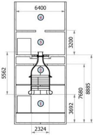
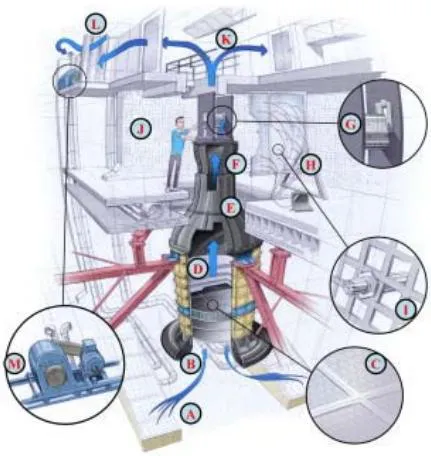
Eg. The David Taylor Research Center planned and developed the Anechoic Flow Facility after realising the benefits of keeping the model and measuring instrumentation still and making the fluid move, as well as the tremendous expense of conducting full-scale tests and the fact that noise reduction is easier with air than with water.

With features like the use of a wide-angle diffuser to achieve a 10:1 contraction ratio without a long diffuser and high-cost return direction. Instead of the more common four 90" turns, two 100' turns and two 80° turns were used. This allowed for the fan noise suppressors to be longer, but with a shorter passage. Noise-reducing fabrics on walls, ceilings, and spinning vanes, as well as very hard concrete constructions. The transparent research section is surrounded by an anechoic chamber, which results in the lowest noise levels ever reached in a wind tunnel. Section separation, as well as the isolation of the entire tunnel from the ground by multiple feet of crushed rock, is used throughout. [10]

Another example of an anechoic or aeroacoustic tunnel is Delft University of Technology's recently refurbished vertical tunnel (V-tunnel), which has been redesigned as a state-of-the-art facility for experiments in aeroacoustics (A-tunnel), as well as fundamental studies in laminar-turbulent transformation and flow control.[14]

(a)

(b) Figure 2: Aeroacoustic Tunnel, Source: [14]

xv. Aquadynamic Flume or Water Tunnels

Water tunnels, are not wind tunnels. However, Water tunnels, are used in precisely the same way as low-speed wind tunnels which work under the same mathematical mechanisms. Cavitation phenomena may be investigated directly in a water tube, which is not possible in a wind tunnel. For obtaining the same Reynolds numbers, water tunnels are physically smaller than wind tunnels. However, the challenge of using water instead of air as the operating fluid more than offsets this obvious advantage. The wind tunnel's aerodynamic rules apply similarly to watercraft, with the exception that water is more viscous and therefore exerts larger forces on the material being tested. For underwater aquadynamic research, a looping flume is often used. Pure wind tunnel research is only partially applicable due to the interaction between two distinct kinds of fluids. A towing tank, on the other hand, conducts related studies. [45, 86]

xvi. General-Purpose Wind Tunnels

Many of the wind tunnels that have since become general-purpose facilities were initially built to meet the needs of experiments on aircraft of the World War I period. The 7 X 10-ft class wind tunnel is the most general, with those estimated dimensions for their test parts. All NASA research centres dating back to the NACA era have or have one or more of the following: The US Air Force has one, the US Navy has two, five US universities have tunnels of this kind, and a variety of other governments and organisations around the world have or have had tunnels of this type.

xvii. Computer Controlled

The following conclusions have been reached after the construction and testing of new computer-controlled wind tunnels:

1. Several different mean wind profiles can be created by individually manipulating each fan, and symmetrical profiles and turbulences can be created both under the ceiling and on the surface.

2. Each fan may be regulated in a periodic or dynamic manner to generate high turbulence intensities and integral scales.

3. It is possible to simulate the necessary atmospheric wind characteristics by systematically manipulating several variables. [12]

d) CFD VS WT

Computational/ theoretical tests or Wind tunnel Test for a model?

In the 1970s and early 1980s, it was thought that the use of wind tunnels, especially in the subsonic regime, would rapidly decline as computational fluid dynamics (CFD) or FEA (Finite Element Analysis) software would become a more cost-effective method for obtaining data for many engineering applications. ([45] Barlow et al. 1999).

Nonetheless, computational simulations have progressed since then, but they are still far from being able to completely replace the need for experimental evidence in development projects. During this period, the computational method will certainly predict basic models such as actual flow in a wind tunnel, but it also takes a long time, making it complex and costly. Furthermore, as compared to wind tunnel results, the computational method also does not have a satisfactory measurement of drag. As a result, wind tunnel testing will continue to be the most popular method for aeronautical growth in the near future. [19, 45]

Matter of fact, the investigative approaches that led to quantitative forecasts were a mix of experiment and theory, with computational methods emerging as a new effective tool in this area. Furthermore, although the utility of CFD methods has increased over time, thousands of hours of wind tunnel testing (WTT) are still needed for the construction of an aircraft, wind turbine, vehicle, or some other design that requires complicated interactions with the flow.

Subsequently, due to the budding attention of other branches of industry and science in low speed aerodynamics, and due to the persistent incapability of achieving accurate solutions with numerical codes, even with advancements, low speed wind tunnels (LSWT) are essential and irreplaceable during research and design. [18]

Many times, when testing new designs and materials, FEA software fails to create the interactions and properties that are unknown, and wind tunnels step in to help produce accurate flow modelling results.

Because of their ability to combine various types of data, wind tunnels prove to be a critical device in the efficient and detailed design procedure of anything that involves fluids. [21]

Thus, across a wide variety of manufacturing and research applications, experimental explorations remain the mainstay for collecting evidence for designers to produce detailed performance and final decisions.

e) Importance

The Wind Tunnel is well-known for its vast potential in civil, environmental, automotive, and aeronautical applications. Everyone's key priority in today's world is to save time, content, and resources, which has forced everyone to opt for preliminary experimentation on miniature models before forming the finished product. One such platform is the Wind Tunnel, which provides us with the ideal atmosphere conditions around the model sized to the required dimensions.[52]

Wind tunnels are a vital instrument in the simple, effective, and rigorous design phase of something that requires fluid dynamics, as well as sharing concepts with peers or clients, due to their ability to merge all forms of data, i.e. quantitative data and visualisation.[47]

Prototypes may also be used for concept checking or recording vast amounts of data in wind tunnels, although the most valuable feature of wind tunnels is that they precisely simulate the maximum complexity of a fluid flow.

Aerodynamic testing has now grown into other areas such as the car industry, engineering, the atmosphere, education, and so on, making low-speed wind tunnel experiments increasingly important.[18]

f) Applications and Other Effects

Technical information for a large number of engineering applications such as external aerodynamics (flow over terrestrial and aerial vehicles), civil engineering (flow over bridges, buildings, cables, etc.), sport activities (flow over cyclists, design of volley and basket balls, wind sails etc.), fundamental fluid dynamics (laminar and turbulent flow over simple and complex geometries) could be aided with Wind Tunnels forming extensive frame of other options in industry and research centres at universities around the world. It can also be used in wind engineering to calculate the velocity around structures, as well as forces or pressures on structures, and to precisely measure the air movement of fans, turbine blades, and propellers.[52]

i. Specific Applications

a. Aerodynamic Applications

Wind tunnels are used by scientists and engineers to investigate the pressures, forces, and air flow direction that impact an aircraft. [23, 45, 47]

b. Calibration

Wind Tunnels are used to calibrate instruments, too.

c. Fluid Flow

Fluid flow researchers have been researching fluid flows in different ways for decades, and fluid flow analysis is still a significant area of study today. Fluid flow is important in a variety of situations. Gaseous flows are observed in the construction of automobiles, aeroplanes, and spacecraft, as well as in the design of turbines and combustion engines. Liquid flow study is important for maritime applications like ship construction, as well as civil engineering ventures like harbour design and coastal defence. Fluid flow in reactor tanks is significant in chemistry, and the flow in blood vessels is studied in medicine. Numerous other examples could be mentioned. In all kinds of fluid flow research, visualization is a key issue. Wind Tunnels are great instruments to visualize flow $[3]$ $[19]$

ii. Non-Aero applications

a. Architecture

In architecture, due to the fact that buildings are placed on the ground and are usually of relatively low height, they are well within the atmospheric boundary layer.

The airflow around large structures, tall buildings, and Office towers with odd or complicated shapes is studied in wind tunnels (such as building with a parabolic or a hyperbolic shape). Aerodynamic assessments of any famous structure, nearly everywhere, are regularly requested by architects. Any construction part must pass an aerodynamic test before being approved for use in hurricane-prone areas like Florida. [45, 18, 19, 26, 52, 85].

EG. [31] Yoshihide Tominaga, Bert Blocken-"Wind tunnel analysis of flow and dispersion in cross-ventilated isolated buildings: Impact of opening positions"-This paper uses a Wind Tunnel to provide a systematic experimental study of cross-ventilation flow and dispersion in five generic isolated single zone buildings with various opening positions.

Aerodynamic influences are substantial in the design of large bridges. Cable suspension bridges or cable stayed bridges are analysed in specialized atmospheric boundary layer wind tunnels.

b. Vehicles

Airplanes

Aerodynamic considerations, with differing degrees of attention to performance, endurance, stealth, acquisition expense, operating cost, time to completion, and any other factor that a customer may need for planned missions, dictate the shapes of aeroplanes.

Another application is the combustion testing of aircraft engines, which necessitates the purchase of an expensive device to purify the air in the tunnel and ensure the same air quality. Another increasingly significant aspect of aircraft construction is their noise footprint, which is usually only tested in a wind tunnel.[18, 19]

Airport Glide Paths

EG:[38] In this paper- Wind tunnel research was performed in Tongji University's TJ-3 boundary layer wind tunnel to analyse the impact of complex terrain on the wind characteristics of the glide paths at Hong Kong International Airport's North Runway. Cobra probes were used to assess the wind speed and direction at the North Runway glide paths. The influence of terrain on wind characteristics such as turbulence strength, turbulence integral size, and mean headwind speed was investigated. The findings suggest that terrain variations have a major impact on the glide path wind characteristics. With the turbulence strength in the wind direction at the same altitude, turbulence intensities in the cross-wind and vertical directions increase; the inflow can affect aircraft landing due to the decrease in headwind speed at glide path 25RA caused by obstruction of certain terrain

The terrain model used was: Lantau Island and HKIA were included in the test simulation set, which was a circular area with a diameter of 27.2 km. The model was produced with a 1:4,000 geometric scale ratio and a diameter of 6.8 inches.

Automobiles

There are millions of cars on the road today that bear witness to the impact of exterior aerodynamics on design decisions. It goes without saying that in automotive applications, the car's aerodynamic drag is important. Despite this, owing to the current high degree of regulation of this parameter, as well as imposed speed limits, the majority of efforts are focused on reducing aerodynamic noise. The ground effect simulation is therefore very significant, which necessitates the use of very sophisticated facilities in the test section to enable testing of both the ground effect simulation and noise generation. [18]

EG. [35] The standard open road simulated configuration is contrasted to simulations in which the computational environment is a computer model of the full slotted wall wind tunnel test segment geometry in this research paper. A sedan-type car is tested in various configurations, and the simulation effects are compared to physical force and pressure measurements. When compared to uncorrected calculation evidence, the results show that simulating the car inside the wind tunnel can predict the absolute drag coefficient with high precision. Despite the high level of consensus for drag, the estimation of lift is less accurate.

F1 Cars

The rising need for fuel in cars necessitates an increase in automotive aerodynamics in order to conserve energy more easily and efficiently. Upgrade pressure on aerodynamics has increased rapidly, especially on F1 race cars. Aerodynamic forces have the ability to drive the tyre force against the road, increasing the vehicle's momentum. A spoiler may be mounted to raise the downward impact. To perform intensive research in developing vehicle aerodynamics, F1 car designers develop their own wind tunnel. One simple way to tackle aerodynamic issues is to use a low open type wind tunnel. [1, 2]

Bikes

Experiments have shown that the amount of wheel spokes and other data affect drag. The use of wind tunnels has proved to be useful in demonstrating to bike riders how to travel with the least amount of drag. [19]

Yachts

Racing-yacht keels are the focus of extensive research in the hopes of gaining a few seconds per mile advantage.

Sails and Above-Water Parts of Ships

Over the years, the efficiency of sails has been tested in a small number of wind tunnels. Sail tests, in general, include measuring side impact, drag, yaw, and roll on a model placed on the tunnel floor in an atmospheric tunnel with a correctly simulated boundary layer.

Rails and Trains

Wind tunnels are employed for testing rail as well as public vehicles of transportation. For e.g. the non-profit Rail Tec Arsenal (RTA) testing centre used Climatic Wind Tunnel located in Arsenal, Vienna to provide climatic validation for rail and public transportation vehicles. This facility had two climatic wind tunnels that could replicate different weather conditions by adjusting temperature, air pressure, humidity, and wind speed. [88]

c. Sports

Wind tunnel testing of athletic goods, such as golf clubs, golf balls, Olympic bobsleds, Olympic cyclists, and race car helmets, has been commonplace over the years. In open cockpit racing cars, helmet aerodynamics is especially relevant (Indycar, Formula One). Excessive lift pressures on the driver's helmet can cause neck pain, and flow separation on the back side of the helmet can cause turbulent buffeting and hence distorted vision at high speeds. [81]

Such initiatives have resulted in significant changes in clothing. Clothing has been tested in some situations to see how it will improve drag when worn by a competitor who wants to increase load during exercise. Vertical wind tunnel training has been given to airborne soldiers so that they are comfortable with the conditions they will face while jumping from planes.

Skiing

For skiers, the "form" is placed in the tunnel and assumes a set of positions during a run at about 55 mph (which is similar to full-scale "flight") in order to learn and minimises his or her drag or perhaps the lift to-drag ratio in the case of ski jumpers.

Cycling Pelotons

EG. [34] In this research, Drag on cycling pelotons was analysed by Wind Tunnel testing of Wind Tunnel Laboratory at the University of Liege in Belgium and Wind Tunnel Laboratory at Eindhoven University of Technology in the Netherlands and CFD simulations were carried out

d. Wind Turbine Testing

WTs are used for testing wind turbines or windmills or for effects of wind barriers on solar collectors being simulated in a wind tunnel[45]

Examples in literature:-

1.[13]In this detailed experiment paper, work was carried out in an atmospheric boundary layer (ABL) wind tunnel to investigate the characteristics of the complex wind loads operating on a standard three-blade horizontal axial wind turbine model in this study. The tests were carried out in a large-scale aerodynamic/atmospheric boundary layer (AABL) wind tunnel at Iowa State University's Aerospace Engineering Department. The test model depicts a wind turbine in a wind farm with a rotor diameter of approximately 90 m and a tower height of approximately 80 m at a scale ratio of 1:350.

2. [27] In this study, the output of a newly developed cross-axis wind turbine (CAWT), which combines the advantages of horizontal and vertical axis wind turbines (HAWTs and VAWTs), was tested in a calibrated open-circuit low speed wind tunnel to match the wind field in an urban environment.

3. [20] Turbulence, one of the most prominent characteristics of urban flows, is investigated in this article, as well as its effect on the efficiency of small VAWTs (often used in urban wind installations). The aim of this experiment is to test an H-Darrieus VAWT prototype in a wind tunnel under various turbulent conditions in order to investigate the effects of turbulence strength, integral length scales, and Reynolds number. The rotor of the turbine was a two-blade H-type Darrieus turbine with two NACA0018 blades, each with a 5 cm chord (c) and two inclined struts.

e. Fan Testing

Wind tunnel experiments are also carried out to accurately determine the airflow of fans at a certain pressure. The standardisation of the data is maintained by assessing the ambient conditions during calculation and then revising the airtightness. [86]

f. Construction Bridges

Natural wind effects are crucial in the proper construction of long or even intermediate bridge spans. At least one event has been recorded in which low-speed aerodynamic excitation resulted in fatigue cracking of high-aspect-ratio beams in a bridge superstructure. Thus it is important to know (1) vortex shedding, which induces minimal vertical displacement or torsional oscillations at low wind speeds, and (2) flutter instability, which may induce both vertical and torsional oscillations.

Roof

EG. [24]Jimmy Colliers' thesis shows how to prototype double curved thin shell wind tunnel structures with incorporated pressure sensors using a prototyping technique. A hyperbolic paraboloid roof structure's development mechanism is depicted. The wind load distributions obtained are compared to literature for a flat roof and canopy constructed using the same technique, as well as two hyperbolic paraboloid roofs. The results show that these thin shell wind tunnel models provide more accurate wind pressure distributions over very thin canopy systems than traditional wind tunnel models. For double curved thin shell wind tunnel models that allow simultaneous pressure measurements over both sides of a thin canopy, the presented fabrication technique for scaled wind tunnel models of glass fibre composite is convenient and precise. The technique can be readily applied to a variety of organically formed membrane or shell structures, and it allows for the use of diverse materials as long as the structure can withstand wind loads during wind tunnel testing.

Low Rise Structures

Important aspects of wind tunnel model simulation experiments of theatmospheric surface layer for the assessment of wind loads on low-rise buildings can be carried out. [29]

iii. Other Applications

a. Multipurpose Climatic Wind Tunnel

The Doriot Climatic Chambers (DCCs) are a pair of very large, extremely advanced wind tunnels/environmental chambers at the Soldier Systems Center (SSC) of the United States Army in Natick, Massachusetts. The Chambers, which were built in 1952, are a one-of-a-kind laboratory capable of simulating a wide variety of global environmental scenarios for both, evaluating military equipment and testing of human physiology, and adaptations in different conditions [89]

b. Environmental Wind Tunnels

There are tunnels that are constructed to mimic Earth's natural boundary layer, which is normally 1000-2000 feet deep. Wind loads on roofs, air pollution dispersion patterns, soil erosion, snow drifts, movement patterns in the proximity of building complexes, and so on are all calculated using them. "Meteorological wind tunnels" is a term used to describe them. The airstream in an environmental wind tunnel is not supposed to be straight and flat, as it is in other tunnels used for vehicle construction tests. To reflect the atmospheric boundary layer, it is instead manipulated to obtain a flow distribution that is nonuniform in time and space. Since the properties of the atmospheric boundary layer vary greatly depending on terrain conditions, the tunnels must be able to adapt the flow to mimic a variety of scenarios. This is achieved by installing customizable roughness elements along the tunnel's floor for up to 10-15 test-section widths upstream of the model's location. The University of Western Ontario's Boundary Layer Wind Tunnel Facility also has an expanded water reservoir for simulating flow in the marine boundary layer. [45, 46]

EG. [15]In this research, analysis and design through experimental and numerical investigations showed that the grid acting as a passive flow control device was effective to reproduce in a short wind tunnel the main characteristics of an atmospheric boundary layer.

c. Wind Engineering

However, over the last two to three decades, the techniques have evolved into increasingly advanced and complex procedures used to cope with highly non-uniform and unsteady flows and their consequences. The computational lexicon has gained a new concept of Wind Engineering. Wind engineering incorporates meteorology, fluid dynamics, structural mechanics, and mathematical analysis to reduce wind's negative effects while maximising its positive ones. In general, four distinct fields are investigated: Wind Forces on Structures and Buildings Forces, moments, deflections, local pressures, and velocities are all involved in these problems.

Static Loads and Associated Experiments on Buildings

Wind tunnel engineers may be called on to help fix structures that have already been constructed and are experiencing problems, or to advise an architect on a new design. House swaying, losing windows or cladding, losing roofing, people being knocked down by waves, whistling sounds, smoke or other gases entering into the air system, and so on are all examples of "trouble." Since the planner is normally very defensive, these experiments are tenser than those on planned houses. It is less expensive to make modifications to proposed projects.

Wind Engineering Example of Wind tunnel-A wind tunnel with two experimental chambers was designed by Diana [82] and can be used for both aeronautical and wind engineering applications. [15]

Flow Over Hills

Example – In [39] an analysis of the precision of a wind tunnel investigation of flow over a dynamic terrain model has been conducted. The Rakaia River Gorge area of New Zealand was modelled both terraced and contoured to an undistorted geometric scale of 1: 5000. Three different surface roughness conditions were tested on the contoured model. Three teams of investigators investigated up to 27 points on either side and inside the river gorge on two spring days chosen for high adiabatic down valley wind flow. Wind speed and direction were measured from a height of 10 metres. Statistical correlation and scatter diagrams were used to equate the laboratory simulation findings to the available field data. The model and field effects were used to evaluate the utility of laboratory tests as part of a plan to establish and demonstrate reliable and cost-effective methods for locating favourable wind energy conversion sites.

Research carried out in

Boundary-Layer Wind Tunnel has a test section 1.22 m X 1.22 m X 12.2 m.

Boundary-layer depth and integral scales are controlled by a combination of square rod grids, fences, and surface roughness.

Unsteady Aerodynamics in Wind Engineering

In a variety of ways, the wind may trigger structural oscillations and other phenomena. The following are few examples of common situations.

Simple Oscillations

Unless critically or over damped, all natural and man-made systems have one or more natural frequencies at which they can readily oscillate. Many things (trees, signposts, etc.) have natural frequencies that are similar enough together.

Aeolian Vibrationsor Eolian

Long, clearly supporting buildings, such as smokestacks and antennas, have a propensity to oscillate at their natural rhythm in a direction normal to a relatively smooth steady wind. The convergence of structural inclination to vibrate at a normal frequency and aerodynamic phenomena of slender bodies shedding vortex streets causes this phenomenon. One of the most discussed problems in fluid mechanics is vortex shedding from spherical tubes. There is an alternating shedding of associated unsteady side force and drag over a set of Reynolds numbers. The shedding frequency corresponds to a Strouhal number of around 0.2 under a broad variety of conditions. As can be shown, there would almost certainly be a wind speed at which the shedding frequency, and therefore the side-force frequency, equals the structure's normal frequency.

There is expected to be a noticeable pulse when such a coincidence happens. This form of oscillation is known as aeolian, though the term is often limited to structures with a high natural frequency (10-100 Hz) and small displacements. The tones in a "Aeolian Harp" created by the wind are generated by such oscillations.

Galloping

A second form of motion occurs where a body's lift curve has a negative angle, and motion through the wind generates a force in the wind's path. This is common in buff bodies whose in-wind side becomes unstilled with a minor angle of attack, allowing Bernoulli-type flow to intervene. Galloping oscillations are commonly aggressive and need design modifications to remove. Twisting stranded wires or inserting spiral wrappings, for example, has been shown to be useful in many situations.

Breathing

Large-diameter stacks and other configurations may also deform at a normal frequency, changing the flow pattern at that frequency. This is distinct from body motion that is free of distortion.

d. Agricultural

Windbreaks

Windbreaks may be used in conjunction with structural load reduction. A second and more critical use is to minimise winter heating loads by lowering a house's convective cooling, and a third is to boost yields from wheat varieties that don't like being blown around. [45]The drag coefficient is a significant indicator of a windbreak's wind protection effect. Although there have been numerous studies on this subject, only a few have included direct measurements, particularly those involving practical windbreaks. Wind tunnel tests were performed on artificial versions of small and practical windbreaks with various porosities. [33]

Windbreaks are used all over the world to change the surface temperature and soil quality for human and animal life as well as crop production. For environmental sustainability, large-scale agroecosystems with vegetative windbreaks have recently been developed (e.g. Wang and Takle, 1997a). A windbreak's main impact is its aerodynamic control on surface airflow, which causes changes in microclimate, soil climate, and crop growth. The windbreak, in theory, acts as a drag on the wind area, creating a net loss of momentum in the incompressible airflow and thus a sheltering effect (Rain and Stevenson, 1977).

As a result, several analyses of windbreak drag and drag coefficient have been conducted.

The configuration of a windbreak, which can be classified into two categories: artificial windbreaks (e.g. thin screens, fences) and vegetative windbreaks, determines the windbreak drag or drag coefficient. In aerodynamic analysis, the former is often constructed with optical porosities and is referred to as "non-thickness." As a result, these windbreaks are often referred to as "two-dimensional windbreaks." The above, on the other hand, has breadth and internal structure.

Agricultural Agronomy

Many agricultural products are pollinated by the wind, so proper plant distribution and planting patterns are important. To boost natural winds, trees on the fields' edges will need to be removed. Some trees, on the other hand, do well without a lot of wind buffering, and these need special care. The application of wind engineering to agriculture is also in its infancy. [45]

Soil Erosion

The agronomist is interested in wind-induced soil erosion because it results in the loss of topsoil. In the other side, the road engineer wants his or her roads to remain open. Windborne particles destroy vehicle windshields and paint, which is another facet of soil erosion. When a stream of wind passes over a bed of loose debris, those higher up create more drag, eventually rolling and bumping in the direction of the wind.

The majority of the motion (and end deposits) that create snowdrifts or soil erosion is caused by this process, which is known as "saltation." The particles bump hard enough to rebound into the stream when the wind velocity reaches about five times the threshold speed, and they are then Ad to be "in suspension." In the presence of dropping debris, saltation and suspension may occur at much lower speeds.

E.g. of WTs for soil erosion

In general, two types of wind tunnels can be distinguished: stationary wind tunnels used for laboratory testing and mobile wind tunnels used for field research. The size of stationary wind tunnels is often restricted due to budgetary and/or logistical constraints, while the size of mobile wind tunnels is often limited due to budgetary and/or logistical constraints.

The challenge of studying natural surface conditions is clearly a drawback of the stationary kind.

Important erodibility characteristics such as crusting and soil composition can't be readily replicated, or can only be done with a lot of work. Mobile wind tunnels, on the other hand, can be mounted on structures in the field without destroying the natural environment, allowing researchers to observe the effects of wind erosion on unique natural surfaces. [45, 32, 33]

Mobile wind tunnels are critical instruments for examining and quantifying wind erosion processes on non-imitated natural surfaces in the field under uniform, quasi-natural wind conditions. On a transect in the Republic of Niger/West Africa, a mobile wind tunnel was built at the IBS of the University of Hohenheim to test wind erosion susceptibilities under various conditions and sediment emission on dominant surfaces created under semi-arid conditions. [32] In a wind tunnel, the proper production of saltation and quasi-natural conditions is often influenced by a physical element known as the Froude number. For all wind tunnels used in wind erosion testing, the inability to generate large-scale eddies remains a challenge.

Snow Drifting

Drifting snow will totally shut down a facility by blocking doors and highways. Fortunately, the problem can be investigated in a tunnel with strong scale correlation. Snow patterns that take years to accumulate (in the Arctic) can be replicated in a matter of hours. Kabayashi, Strom, and others offer in-depth studies of the snow-drifting phenomenon.

Evaporation and Related Issues

The growing need to understand plant transpiration and evaporation from open bodies of water has contributed to the creation of wind tunnels in which the moisture content and temperature of the air can be regulated. Tunnels of this kind can be found in Japan, England's University of Nottingham, the United States' Colorado State University, and elsewhere. Both of them are low-speed tunnels with balanced air exchange.

Pollution Dispersion

For all of the different kinds of contaminants released into the air, it's important to understand not just where they'll go, but just how far they'll have to go before absorption decreases their concentration enough to make them harmless. The sheer number and variety of contamination issues is mind-boggling. Industrial smoke, waste gases from chemical processes, efflux from nuclear power plant holding tanks, using wind to carry silver iodide aloft to increase the likelihood of rain, the necessary distance from a liquefied petroleum gas (LPG) spill to obtain a non-combustible mixture, getting rid of hydrogen sulphide smell from a geothermal power plant, and pesticide dispersal through the atmosphere are only a few examples. Furthermore, a full variety of 'weather scenarios must be considered, as well as the worst-case scenario that is "likely" to occur. Skinner and Ludwip made significant contributions to wind tunnel dispersion experiments.

Eg[37]Wind Tunnel and Numerical Simulation of Pollution Dispersion: A Hybrid Approach by R. N. Meroney.

III. CLASSIFICATION

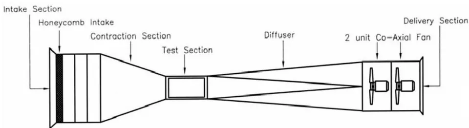
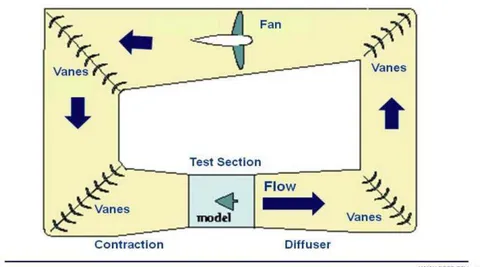
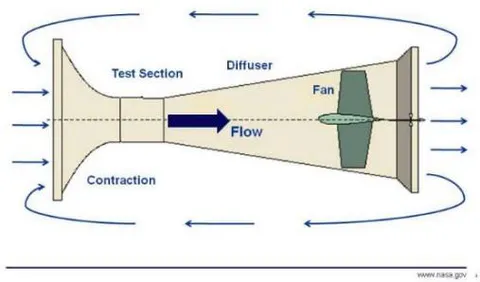
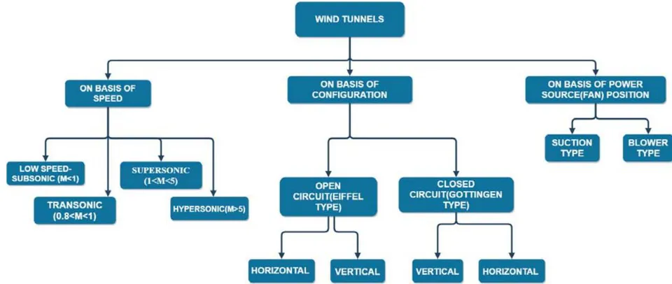
Wind Tunnels can be classified on a variety of basis [5, 8, 9, 14, 19, 23, 44, 45, and 52], such as Based on Design/ Tunnel Geometry: They can be-Closed/ Gottingen Type or Closed circuit (CCWT) (Return loop of air fed back, closed and re-circulates the air through the test section) and Open/Eiffel or Open Circuit (OCWT) (No return loop, open on both ends and draws air from the atmosphere into the test section)[8, 14, 44,19, 52]

Based on Velocity/Speed configurations or Mach number: They can be subsonic/ low speed/ small (M < 0.8), transonic (0.8 < M < 1.2), supersonic (1.2 < M < 5.0), or hypersonic (M > 5.0). [23, 45, 19, 52].

Based on the test section of the wind tunnel itself: can be either enclosed by physical boundaries (Walls) called closed-jet or open (so called "open-jet" wind tunnels) or Semi-closed.

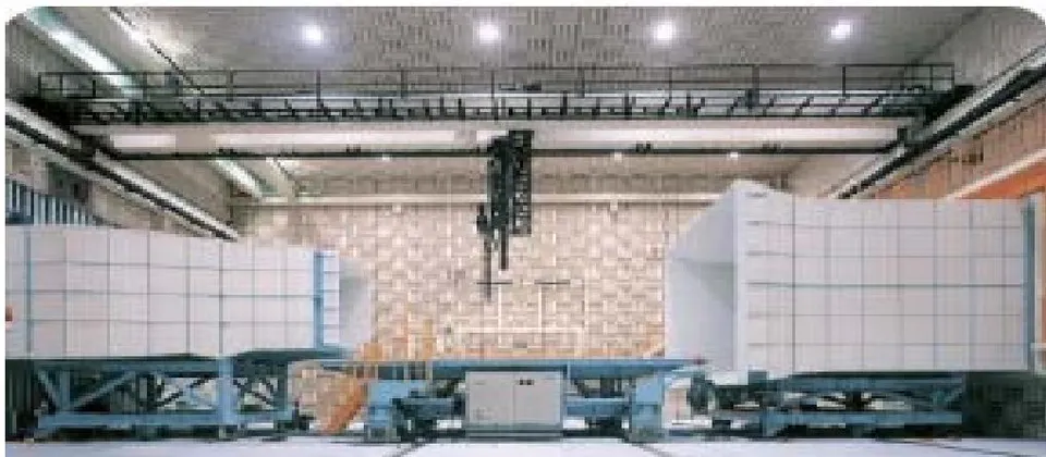
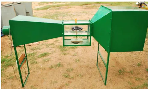
Based on position of fan housing and diffuser: when it is placed at the end, it is called "Suck Down" whereas if it at the start, it is called "Blower" configuration

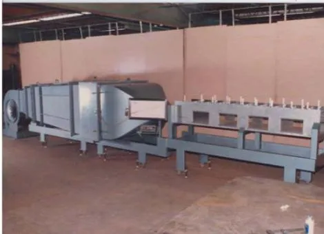
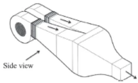
Apart from this basic classification, wind tunnels can be classified as, [26]

1. Based on structure—funnel shaped or normal type, horizontal or vertical axis wind tunnel, long, short or medium length wind tunnel

2. Based on structure material - Metallic structure or concrete type or composite structure wind tunnel

3. Based on shape of inlet section - Semi-circular, circular, square, semi-elliptical or other cross sections of various shapes

4. Based on location- outdoor location or indoor location wind tunnel

5. Based on anemometer placement - push in type, windows for anemometer, anemometer frame type.

6. Based on mode of operation - Pressure storage, in-draft or Pressure vacuum type. [23]

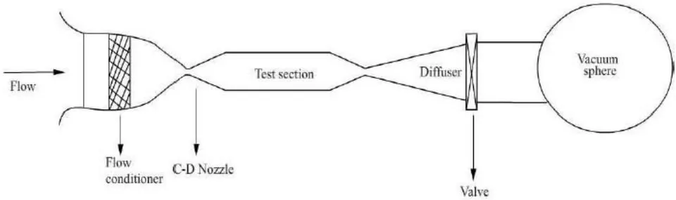
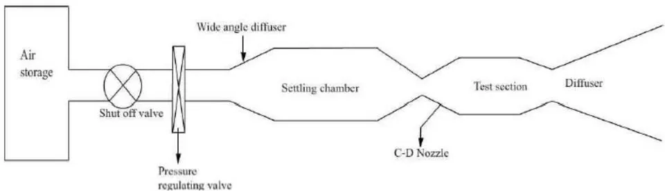
7. Based on Operation - Continuous (for all speed ranges) or Intermittent; With increasing Mach number the tendency to intermittent operating wind tunnels linked with an appropriate energy storage arrangement, becomes more and more compelling. However, for measurement of low subsonic flow, the continuously operating wind tunnel is more preferred. [9]

a) On the basis Design/ Wind Tunnel Geometry

In particular, the type of tunnel preferred is determined by the amount of resources invested and the intention of the project.

Closed Circuit Wind Tunnel (CCWT) or Closed Return Wind tunnel or Gottingen/Prandtl type:

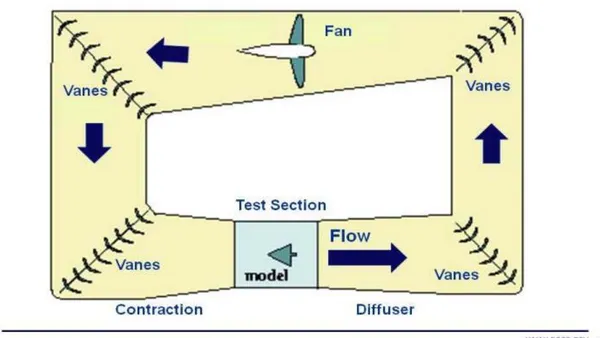
Closed circuit wind tunnels provide a closed loop (feedback) of the airstream in which exhaust flow is directly returned to the tunnel inlet, avoiding unnecessary power losses and increasing total performance of the system $[47]$. Closed circuit tunnels produce a steady air mass and do not account for leakage. To achieve a regulated return flow, the most high-performance wind tunnels were configured as closed-circuit types.

To cut down on the amount of energy used, a closed circuit tunnel has been established. Prandtl pioneered this category of wind tunnels in Göttingen, Germany, and thereby the name $[50]$. This tunnel's main function is to circulate used airflow from the diffuser to the settling chamber through the connecting channel and corner vanes. In an enclosed loop, air is recirculated. They take up so much room and are more difficult to build and manufacture. (43, 45) It's also possible to use a cooling system. [10]

There are two kinds of closed circuit tunnels: single, and double return. Only the first of these is currently widely accepted. The air that scrapes along the walls of the return passages forms wakes in the centre of the jet and hence flies directly over the model in the double return arrangement. Unless the contraction ratio is high, the air is highly turbulent, making it impossible to interpret the test results. The fans are preferred to be connected to the connecting channel because it defends against model loss and increases fan performance. [7, 9, 14, 19, 47]

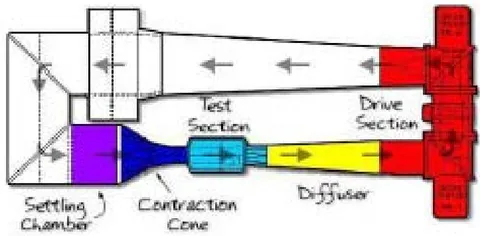
As stated above test section could be:

Open Test Section: Air is blown from the contraction cone to an open space between the contraction field and the diffuser in this location. Here is where the test method is typically mounted. This form of test section results in a significant amount of pressure loss. The creation of a jet-shear layer from the nozzle's exit characterises a wind tunnel with an open jet. As compared to their closed-section counterparts, the jet exits in a comparatively wider domain, which reduces the aforementioned wall effects and decreases background noise levels. Measurement instrumentation is also less invasive, owing to the open jet's flow and optical accessibility, which enables instrumentation, such as microphone arrays, to be positioned outside of the flow. However, because of the jet spreading and model circulation, flow consistency and synchronisation are more difficult to monitor, necessitating extensive corrections to achieve the effective angle of attack and effective aerodynamic coefficients. [14]

Closed Test Section: The contraction cone has air blown into a closed wall test segment here. This section, closed by walls is normally where the test model is kept. Wall friction is caused by the test section's walls. [44 and 50] A wind tunnel with a restricted testing region allows for a faster reconfiguration of the freestream flow, resulting in lower model blockage and airflow corrections and more closely regulated aerodynamic properties [14]. Erroneous readings of the sound frequencies produced by the model can be induced by high background noise levels [16] and reflections from the solid surfaces of the test segment.

To optimise uniformity in the return flow, CCWTs must be strategically crafted. Axial fan(s) are used to operate these tunnels upstream of the test section, and multistage compressors are often used to produce trans-sonic and supersonic air speeds. [47]

Plus points

1. Quality of flow can be well controlled by suing corner-turn vanes

2. Quality of flow is also independent of weather/outdoor conditions as well as of other activities in building

3. There is lesser noise during operation

4. For a given test section size alongside velocity, lesser energy is required, since there is decrease in the pressure and power losses. This is really helpful for a tunnel used for development experimentation with a very high usage rate (2, 3 times for 5, 6 days/week). [21, 45, 9, 47, 7]

Drawbacks

1. A huge amount of initial investment (due to return ducts and corner turning vanes)

2. There exists a necessity to purge the tunnel, if smoke or other flow indicators are used, as there could be entrapment of the same.

3. A technique of cooling would be mandatory for high utilization of the tunnel. [21, 45, 9, 47, 7]

Open Circuit Wind Tunnel (OCWT)/ Eiffel Type With an Open circuit wind tunnel, it is possible to achieve high performance, and even save space and construction cost. In essence, an open circuit wind tunnel is actually a closed circuit wind tunnel with a shabbily designed return leg/lag. OCWTs keep replenishing or keep cycling fresh fluid/air. It requires a pre requisite amount of free room around for no effect on quality of return flow. Its specific design was pioneered by French engineer Gustave Eiffel in 1909, hence the name, "Eiffel Wind Tunnel". This classification consists of an Intake, a nozzle/contraction, test section, diffuser and a driving unit/ exhaust with no corners nor long diffusers [9, 45, and 50]. It lacks any loop feedback. This category of wind tunnels is generally used in spacious, closed rooms in order to reap the benefits of natural feedback air [7, 10, and 43]

Principle working of OCWT, is the direct sucking of external atmospheric air brought into the settling chamber with an end to the air's journey by a driving unit or exhaust lying on extremity, and then thrown away to the atmosphere.

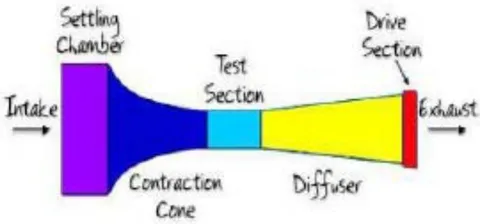
The drive units may be placed at the tunnel's downstream end, where it is run as a suction tube, or at the tunnel's upstream end, where it is operated as a blow down tunnel. Because of the consistency of the airflow, the suction tunnel is favoured in a configuration. [9, 19, 50, 10, 7] That is, the Open circuit wind tunnels are further classified as:

i. Blow down configuration or Blower configuration

The blower creates a high pressure at the inlet, allowing for significant shifts in operating section configurations. Since the fan is at the inlet, the exit diffusers may be skipped (at the expense of power loss) to allow entry to the test section without upsetting the flow. Blow down tunnels are also termed versatile as test models may also be changed to match the scale of the test object. They are referred to as "free-jet facilities." [45] Some Blower configuration employ diffusers at the start of wind tunnel which could be one or even two in number

ii. Suck down configuration

Suck down wind tunnel creates a pressure drop at the tunnel's exit, allowing airflow to flow through it. The diffuser and fan housing is usually at the end of the Wind tunnel. The return flow of suck down tunnels is vulnerable to unpredictability. However, since the air does not flow through the blower until hitting the test, the blowing impact, and swirling effect of the air is minimised. The only benefit of a suction tunnel with a centrifugal or axial fan at the exit is the questionable claim that air from the tunnel room may be less disturbed than air from a fan. [9, 47]

1. The main advantage of open-circuit tunnels is in the saving of space and cost.

2. They also suffer less from temperature changes (mainly because room volume > tunnel volume) and the performance of a fan fitted at the upstream end is not affected by disturbed flow from the working section.

3. They can be used to run internal combustion engines and extensively use smoke for flow visualization without the need to purge. [21, 45, 9, 47, 7, and 52]

4. Its Set-Up and Maintenance Cost, which is very small as compared to CCWT.

5. The leading manufacturer of automobiles utilize the OCWTs for the Drag and performance estimation of the vehicles since, with current tech & blueprint designs, these tunnels give results quite close to practical values under proper calibrations.

Drawbacks

1. Since, they are open to atmosphere, the pressure (mostly static pressure) is usually greater than atmospheric pressure in regions of high air speed. This implies when an OCWT with an exit diffuser is used, it gives rise to spurious jets issue from holes remaining unpatched, that is, leakage is unavoidable due to holes often drilled for mounting probes and models in test section [19, 46]. This is often minimized by impeding the outlet or by creation of an overpressure in the working sections.

2. OCWTs can be noisy if tunnels have larger test sections like 70 sqft or more. The noise causes environmental issues, it limits the hours of operations and mandates the use of sound proofing equipment or noise treatment of tunneland surrounding room.

3. In order to achieve extreme high quality flows, extensive screening at the inlet might be required, especially if the tunnel is within a room depending on size of tunnel to room. An alternative to controlling the flow conditions (temperature and relative humidity) is housing the wind tunnel in a large closed room with an HVAC system that has a larger capacity than the load imposed by the wind tunnel.

4. OCWTs would need higher energy to run, which is a contributing factor to the high utilization rate in developmental experiments [21, 45, 9, 7, 47, 10]

5. They are generally placed in large rooms, as are sensitive to impediments in room, like furniture or walls which give rise to adverse effects in flow.

b) On the basis of Velocity/Speed configuration or Mach number

Small WTs/ low speed WTs/ sub-sonic WTs

They are the most common type with the flow velocity Mach number range of zero to 0.4. In them, viscous and inertial forces are dominant while compressibility effects are negligible. [19] They possess maximum speed capability up to about 300 mph (440 ft./sec, Mach = 0.4, 134 m/s, 261 knots). [45]

High Speed WTs

The designation high speed usually includes:

1. High subsonic

2. Transonic

3. Low supersonic regimes

The range of the flow velocity for high speed wind tunnel is of Mach number between 0.4 and 1.4. Here, in principle, compressibility effects dominant [19, 23]. Also, the viscous effects come to light particularly when shock boundary layer intersection leads to flow separation.

Transonic

Occurs for Mach number nearly equal to one, wherein the speed of air approaches the speed of sound; M=1. [9] Transonic wind-tunnels are common in the aircraft industry since most commercial aircraft operate in this regime.

Supersonic wind tunnel

The flow velocity in supersonic wind tunnel is the range of Mach number between 1.4 and 5.0. Compressibility effects are primarily dominant. The pressure disturbance surges in the flow field propagating downstream. Supersonic wind-tunnels are effectively used to investigate the behaviour of jet engines and military aircraft.

Hypersonic wind tunnel

The flow velocity in hypersonic wind tunnel is of Mach number above 5.0. Real gas effects are desired which require high Mach number in test section along with total temperatures. The high temperatures, linked with high pressures, give rise to vibration of the gas molecules, possibly causing dissociation and ionization. Thus, these are prevailing characteristics of hypersonic flows where the gas can no longer be treated as an ideal gas. [9] Hypersonic wind-tunnels find their applications in rockets and space vehicles.

c) Reasons for Selection/ Design Considerations

An important consideration to take into account is whether the wind tunnel should be closed circuit (return) type or Open circuit (non-return) type. Most of the research facilities which are small-scale and bound by financial considerations implement the open type wind tunnel. Moreover, schools and universities prefer an Open circuit Wind tunnel to assign their course work peculiarly for subjects like fluid mechanics or aerodynamics. Science fair participants who build their own wind tunnels, implement the open design, due to low utilization rates. Thus, the low initial cost, lesser maintenance drove the choice towards an open circuit tunnel.

Moving on, closed test sections are better for measurement and Suction OCWT introduce less swirl. For most of the tests, subsonic, low speeds are enough with axial fans.

Thus, we have chosen a subsonic/low speed OCWT (Eiffel Type) as prime design.

IV. PRIME DESIGN

a) Difficulties in Design

Since the 1930s, when the powerful influence of free-stream turbulence on shear layer behaviour became evident, focus has been placed on wind tunnels with good flow uniformity and low levels of turbulence and unsteadiness. However, due to a lack of understanding of flow through the different tunnel components, it has been difficult to formulate firm rules for wind tunnel construction. Bradshaw and Pankhurst (1964) [45] made the first attempt at presenting some instructions for the complete design of low-speed wind tunnels, and later theoretical tests of flow through individual components of a wind tunnel by Mehta, 1977, 1978 and Mehta and Bradshaw, 1979. [7, 14] For the most part, this has culminated in a deeper perception and design theory. Over the years, the topic has gotten a lot of coverage, with around 50 articles citing specifically the design of various forms of Wind Tunnels. Rae & Pope (1984), a detailed study on the German-Dutch Wind-tunnel written and curated by Seidel, are two books and articles on the subject (1982).

However, wind-tunnel architecture is a complicated field covering multiple areas of fluid dynamics and engineering, and it is difficult to address all of them in a single article. [47]

It is a herculean task to devise prescriptive guidelines for wind tunnel design a priori (Latin for previous/scientifically) due to the vast range of tunnel designs and a lack of knowledge of flow through wind tunnel constituents such as the wide angle diffuser, mesh panels, and the blower/diffuser itself. [8][44]

Manufacturing costs and vibration in each portion due to high wind velocity are just a couple of the drawbacks. An axial fan induces a swirl. When this wind whirl goes into the wind tunnel, it has a different effect on the airfoil. In terms of wind speed, choosing the form and scale of a wind tunnel is a task in terms of engineering and fabrication. [30][7]

Based on data from successful prototypes and some initial studies, we have attempted to present our design specifications for the key components of a wind tunnel—the power source, contraction chamber, settling chamber, and exit diffuser.

b) Guidelines for Design

Crucial Parameters and Main Specifications

The flow quality within the test chamber, as well as the overall performance, are important characteristics of wind tunnels. The flow quality (described by turbulence and flow uniformity) must be specified according to utilization of wind tunnel. Flow quality is a result of design, and can be verified only during calibration tests. [45, 18] It is crucial to avoid flow separation close to the walls of the contraction zone.

Thus, theoretical maximum speed, flow uniformity, and turbulence rates are the three major parameters that are widely used to typify them $[18]$. The main specifications would be the dimensions of test section, along with required maximum operational speed. It has been found that lesser the turbulence, better it is to simulate flight conditions. $[47]$

Other Factors

When the parameters are finalized, it is important to find a balance between overall dimensions of wind tunnel, their compatibility with available room with the overall cost. This cost is dependent primarily on external shape of wind tunnel, and power plant (Fan) requirements. Other parameters to confirm with are, manufacturing process, future possible improvements, and operational/maintenance expenditure for the equipment $[10,17,18,21]$. Energy ratio is the ratio of power (in test section) to flow losses (around the circuit) and is a measure of energy efficiency of wind tunnel. It is nearly always greater than unity for closed as well as open circuit wind tunnels except for free-jet facilities.

Design Aim

The design aim of a wind tunnel's configuration is to achieve a regulated flow in the test chamber whilst preserving flow performance and quality parameters.

Overall Aerodynamic Objective/ Project Scope

The below are the key goals that we want to accomplish with this working model:

1. Build a small scale wind tunnel using different criteria for educational and scientific purposes.

2. To simulate the velocity profile or fluid flow around a scaled model or test piece.

3. Determine the lift and drag coefficients for various test sections' particle velocities.

As a result, most wind tunnels' ultimate aerodynamic aim is to create a flow in the test section that is as similar as possible to a constant steady flow with consistent speed in the test section. Since perfection is difficult to achieve, any design is constrained by factors such as maximum cost, limited space, available time, and available information. For the available funds, it is almost always preferred to achieve the largest test portion and the fastest speed possible. Of course, high speed and huge scale are opposing demands. The cost of the tunnel shell and the power it requires tends to rise with respect to square of the test section width. [45]

Note:

In order to achieve a uniform flow in the test segment, there should be a seamless transition from the contraction section to the test section. At the end of the contraction section and the beginning of the test section, there should be a zero slope to achieve this. The velocity that the architect expects to be obtained in the test parts must first be determined, and then the continuity equation will be used to determine velocity at any cross-section of the wind tunnel. [8]

This paper focuses on the project of suction-type, Open (Eiffel Type), subsonic Wind tunnel but most of the information could be pertinent to wind tunnels in broad-spectrum. This selection pertains to optimal flow quality, while keeping the overall tunnel size limited to any allocated laboratory space.

Components

The main segments/portions/sections of an Open/Eiffel Wind tunnel are

1. Entry Section or Settling Chamber Consisting of a. Honeycomb Meshes

b. Screens

2. Contraction section, also addressed as Effuser or Contraction Nozzle, some authors also use, Nozzle

3. Test Section

4. Diffuser

5. Driving System (Power Drives, e.g. Fans)

The Entry Section or Settling chamber helps make the air flow laminar as well as subdues the transverse velocity component. It achieves this via a Honeycomb Mesh (eliminates uneven flow due to fan) and a series of screens (Provides uniform steady flow). What follows next is the Contraction cone/section (Effuser/Nozzle) whose main objective is to propagate the flow to required velocity for the test section without generating turbulence, but with gradual reduction in area. The test section is that portion, where the aerodynamic model to be experimented/tested is placed, along with instruments for measurement and sensors for analysis. The next section is the diffuser, it helps to regulate, steady and make the flow consistent by maintaining constant air speed in test section. The final section of the wind tunnel is the fan and it's housing, also called, power drive or drive system which is the primary source of wind, drawing air into the wind tunnel, by expelling air out, thus, reducing turbulence and providing greater control of air velocity through the tunnel. [9, 18, 30, 43, 47, 52] In wind tunnels, the chief drive systems found could be: Compressor driven or Fan. Compressor (generally from storage tanks) through a meticulously monitored valve/ regulator supplies pressurized air to the tunnel, in the former, whereas for the latter, Fans/Blowers are employed, which are either shaft or belt driven (depending on cost and sought after performance characteristics). [10]

Compressor-driven facilities could deliver large pressure ratios for relatively little cost but are time and again preferred for high-speed facilities that require high stagnation pressures. Fans tend to work best with low-speed facilities.

Hence, Fan Drive System is chosen as the prime source of power.

Settling chamber

It is region designed to deliver controlled quality flow to contraction cone by diminishing the various flow constituents accountable for turbulence. It makes the flow straight, parallel, uniform and subsides transverse velocity component of incoming air. Itencases, houses/utilizes Honeycombs, Screens to achieve that. Individually used, these sub-sections produce pressure loss, and hence, to obtain better flow characteristics, combination of both are used. The configuration which is found optimal is honeycomb located upstream with one or two screens, following them. [5, 9, 10, 18]

The irregularities of flow found in Wind Tunnels are:

1. Spatial non uniformity- When mean velocity is not uniform over cross section. This could be avoided by transfer of excess total head from high velocity regions to low velocity ones,

2. Swirl- When Flow rotates about an axis causing variation in direction of flow. Flow straighteners like honeycombs help reduce swirl. [10]

3. Low frequency pulsation-There are rapid increments of mean velocity. When occurred, time taken for balanced flow to happen becomes large. The source of such pulsations are challenging to locate. [23]

4. Turbulence- Generates small eddies of different sizes and intensity and causes time variations of velocity. When asymmetrical fluxes are superimposed on mean flow it is defined as turbulence

To reduce these flow irregularities, the settling chambers implement flow straighteners called:

i. Honeycomb

They aid to diminish tangential velocity of the airflow caused by the axial fan by rendering air filaments parallel and levelling the flow. It reduces the radial component of large scale turbulence, that is, vorticity as well as swirl of the incoming airflow $[10,14,23$ and 45]. Hence, their function is to align/even the flow with respect to the axis of wind tunnel and eliminate large-scale flow unsteadiness $[9,10]$. Flow uniformity as well as turbulence intensity in test section is pioneered by honeycomb mesh. This section must possess sufficient structural rigidity, without any deformations, to withstand force during operation. This is because if Mach number of flow incoming is large, it may lead to choking the flow. $[10]$

Mehta and Bradshaw [4, 7] cite the use of 150 cells in mesh per chamber (settling chamber) hydraulic diameter Dh. (around 25000 in total, are adequate, as the cell size is generally smaller than the minutest lateral wavelength of velocity variation)[44, 47]

The authors also profess/insist that to avoid stalling of honeycomb cells, which reduce their efficiency as well increase pressure loss, the yaw angle of incoming air, must be lesser than 10 degree. [5, 7, 10]

The various cross-sections of honeycomb cells could be circular, triangular, square (fabricated due to ease of construction [7]) and hexagonal. The hexagonal shape of honeycomb cell is optimum, as it has the least pressure drop coefficient.[10, 45]

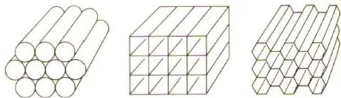
Design parameters for honeycombs are ratio of stream-wise length to single cell hydraulic diameter, and the porosity/solidity.[45]The length of the honeycomb section should be smaller than the smallest lateral wavelength of velocity variation is recommended by [4, 6, and 10]. Optimum performance exists when the length to diameter ratio is between 6 and 10. Also, from studies [4] [5] [6] [7], it has been found that cell of honeycomb of length (thickness) 5-10 times the diameter (cell width or diameter) terminates the lateral turbulence[5, 23, 44, 47]. Porosity is generally in the range around 0.8 leading to honeycomb loss coefficients to low value of 0.5. [45]

Honeycombs are effective flow straighteners, but not that effective as screens to even non-uniformities in flow speed. [18] They are not proficient at minimizing lateral turbulence, moreover, induce axial turbulence of size equal to its diameter, which limits/confines the thickness attainable for honeycomb.

ii. Screens

Screens help increase uniformity of the airflow, as faster flows have higher pressure drops than slower flows. The purpose of the screen is to subdue the turbulence levels of incoming flow, and destroy large number of turbulent eddies into smaller ones which eventually decay $[9,10]$. The scale of eddy decay depends on the Reynolds number of flow which in turn is influenced by the wire diameter used for screen constructions. Screens impose a static pressure drop proportional to the square of speed, increasing the ability of the reducing boundary layer thickness to endure the pressure gradient $[2,5,7,\text{and }18]$. Just a single screen reduces pressure grad by 0.5% which is reasonable for some aeronautical purposes. Screens are sometimes, even tensioned before flow start. When RE<40, eddies are practically absent. $[23]$

These screens are square/rectangular generally constructed interweaving metal wires, nylon or even polyester threads. The gauze action of screen as well reduction in turbulence is effected by:

1. Pressure drop coefficient $K=f_1(\beta ,R_E,\theta )$ {Function of open-area ratio $(\beta ,\beta ={(1-\frac{d}{l})}^2[23])$, Reynold's number $(R_E)$, and $\theta$ which is flow incidence angle measured normal to the screen) K also depends on density, kinematic viscosity and mean velocity of fluid. Non-uniformities in the flow (caused by generation of tiny vortices and random coalescence of small jets emitted by the screen) occur for the screens with low open-area ratios. That is why, at least one screen (generally last) possess open area ratio of

2. Deflection coefficient $\alpha =f_2(\beta ,K,\theta )$

The basic parameters to typify screens are "Porosity" (B), "Wire Reynold's number" (R) and the "Mesh factor" (K). Mesh factor differentiates smooth and rough wire (screen material could be different), they were given by Idel'chik as 1.0 for new metal wires, 1.3 for circular average metal wire (smaller meshes are mostly preferred) and 2.1 for silk threads [45]. Porosity is a function dependent on wire diameter, weave density, and geometric factors. It is the given by the expression

Where, B is porosity,

$d_w$ is wire diameter, $\rho$

$=\frac{1}{w_n}$ is the mesh density, $w_n$ is width of one square mesh

The complement of screen porosity, known as screen solidity is also cited by many authors which is given by: 1-B (1-porosity). Porosity is 0 for packed weaves and 1 for vanishing screen.

Frontal area of the screen should not exceed 40% of cross-sectional area of settling chamber to ensure flow stability. For turbulence reduction, screen used should have porosity greater than 0.57, and it should be noted that screens with smaller porosity suffer from flow instability that acts in the test section, later. [45].

To achieve lowest turbulence in the test section, multiple screens of different porosities could be positioned, with the coarsest screen closer to the incoming flow and the finest screen nearer to test section, along with some free section to decay the variabilities/fluxes created by screens, themselves $[7,9,$ and 10](Watmuff, 1998). The turbulence reduction factors are a product of the individual screens, while the pressure drop is sum of the pressure drops of individual screens, when multiple screens are implemented.

The only issue with screens is their capability to gather dust/dirt, and dust always possesses a non-uniform distribution. This changes the screen porosity, the pressure drop, influencing the velocity and angularity distribution in test section, in an erratic manner with time. This problem intensifies when flow-visualization techniques of china clay, oil (vaporized), and smoke are used. Therefore, screens must be mounted in a manner that they can be later cleaned, and quality of flow in test section must be monitored for the same.

The screens do not considerably impact the lateral turbulence and rather are pretty efficient at reducing longitudinal turbulence. [18] This gives rise to lateral turbulence being less attenuated in contraction chamber. A single screen reduces the longitudinal turbulence level radically, however implementing series of 2, 3 screens attenuates turbulence level in two directions up to $0.15\mathrm{\%}$. Spacing flanked by the screens (between them) should be adequate so that flow pressure has fully recovered from the disturbance (i.e. $\mathrm{dp}/\mathrm{dy}=0$ ) when the flow passes through them, moreover, they generally should lie in the order of the length scale of large energy containing eddies [10]. An ideal spacing of 0.2 times settling chamber diameters (or $0.2D_H$ ) was suggested [4, 5, 7, and 47]. Additionally, the spacing between the last screen and the contraction entry should sldo be 0.2 cross-section diameters ( $0.2D_H$ ). [18, 4, 5, 7, 14]

If the Reynolds's number is based on screen wire diameter, it should, preferably, be lesser than $60\mathrm{\%}$ to prevent additional turbulence due to vortex shedding, as suggested by Schubauer, Spangenberg and Klebanoff (1950).

Contraction Cone/Nozzle/Chamber (Effuser or Node)

A vital component of all wind tunnels, and the most significant single parameter in design having the highest influence on flow quality of air-flow in the test section, is the contraction nozzle/cone/chamber (also called Effuser or node by certain authors $[5]$ ). In spite of the usage of the term "nozzle", contraction cone is never conical in shape. They are primarily attached upstream in the wind tunnel $[2,4,8,18,6,\text{and }45]$

With shrinkage of flow area along the length, the contraction component proliferates/escalates the airflow speed prior to test section entrance $[5,10,and51]$. (It abates/curtails both mean and fluctuating velocity variations to minor ratios of the average velocity while increasing the corresponding mean velocity) $[7]$. It serves a few purposes:

1. It facilitates low velocity at a location where, screens are placed. This low entrance velocity is preferable as it reduces pressure loss in wind tunnel.

2. Mean and fluctuating velocity variations are diminished to smaller fractions of average velocity as stated above.

3. Tones down the spatial variations of velocity in Wind tunnel cross section [23]

4. Subdues flow turbulence and non-uniformities, according to Derbunivichet al. (1987), as well as accelerates, and aligns the flow into the test section [10, 21]

The key parameters of influence are: Contraction Ratio (C.R., ratio of inlet and outlet areas), Shape of Wall/Degree of curve of Wall, Contraction Length and shape of Contraction. For designing subsonic/supersonic wind tunnels, it is paramount that the contraction portion shouldn't possess adverse pressure gradient in stream, and effect of the same at exit of contraction section should be insignificant. [6]

Tennekes and Lumley (1972) stated via their research that, vortex filaments are overextended in contraction section, which consequently, reduces axial fluctuations, however, the lateral turbulent fluctuations are strengthened. Contractions are less proficient in subduing longitudinal turbulence than mean velocity variation for axisymmetric contraction, was derived in rapid distortion theory by Batchelor (1953). [7, 9, 10 and 21]

Contraction Ratio (C.R.)

The Non-uniformity reduction, as well as flow acceleration are governed by ratio of cross-sectional area of Inlet to outlet, designated as "Contraction Ratio". (Deemed as "N" or "C.R", even "q" is found in research literature) In theory, value of N should be large enough to destroy axial fluctuations in the flow, increase efficiency and foster the air in the test section to propagate slower relative to air in the test section [46], but practically, N possesses an upper limit, since, it intensely effects the Wind Tunnel's overall dimension, driving the cost upwards [18]. Thus, a compromise for this parameter is vital, conditional to anticipated applications.

Typical C.R.s found optimal are between 6 and 9. [2, 7, 8, 9, 14, 46 and 47]. For civil/industrial applications, contraction ratios between 4.0 and 6.0 are sufficient to reduce flow turbulence and levels of non-uniformities to order of $2\mathrm{\%}$, which is also adequate of other applications

Cross Section Shape

Another stricture/constraint to be chosen a priori is Shape of cross section of contraction. The optimum cross sectional shape speculated is circular, the reason being, the low velocities encountered in the regions where surface streamlines intersect and separation of corner flow occurring for non-axisymmetric nozzles. Additionally, crossflows and secondary flows arising in corners of polygonal cross sections. [7, 45] Hence, many of the early designs implemented, were circular or octagonal cross sections (Octagonal ones, are achieved using a 45 degree fillet at nozzle start and carrying that throughout the test section and diffuser [45]).

However, later, began a compromise between rectangular, square and circular due to insights provided by Mehta Et.al., 1978, [7, 14], who showed that even for square or rectangular cross-section, corner flow traits remain confined, and these do not drift to affect test section wall flow. Thus, the cross-sectional shape that may be employed could be chosen to match tunnel components, especially the test section [7], which is usually square or rectangular [5, 9, and 51].

Contraction Chamber Curvature-Degree of Curve (Shape of Wall)

Various authors enunciate/articulate different degree of polynomials for the longitudinal-section silhouette/boundary.

Bradshaw et.al. [45], recommend contraction curve to reach $1^{st}$ or $2^{nd}$ derivatives at inlet and outlet by implementing two segments of $3^{rd}$ degree polynomial curves of contraction wall. [16-20, 49]

Most of other authors [4, 7, 14, 18, and 43] suggest a $5^{\text{th}}$ or $6^{\text{th}}$ order polynomial as it satisfies most of the requirements discussed above. Moreover, because these curves give reasonable Reynolds number, flow uniformity and are free of separation (On centreline as well as in corners), they are better than first variation stated above at operational conditions such as $15\mathrm{m}/\mathrm{s}$ velocity. Bell and Mehta also, devised their Bell-Mehta fifth order polynomials for the curvature [51].

Hence, a $5^{th}$ order degree of curve wall shape is optimum for walls of contraction cone. A research for design and optimization of contraction with the help of conic section theorems [5], suggests even a sixth order polynomial with seven parameters. [83, 84]

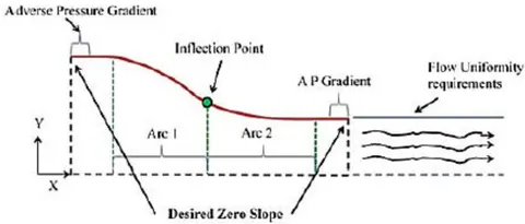
Contraction Semi Angles and radius of curvature

For tunnels with low speed or laminar flow, escalated rate of growth of boundary layer thickness is observed causing centrifugal instability, leading to slow acceleration too, when the radius of curvature is huge, at the upstream end. Thus, the nozzle is fabricated either by method of "Design by Eye" or by alterations of fairly accurate methods, which insists that the radius of curvature should be lesser at the exit rather than the entrance. [6, 45].

The contraction semi-angles: $\alpha /2$ and $\beta /2$ are suggested to be in the range of ${12}^{\circ }$, this allows the contraction cone to retain a judicious length and a decent fluid dynamic behaviour. [5, 18]

Parameterization of contraction profile/curve

If a coordinate system is defined at the origin of the wind tunnel's centre line of contraction inlet plane where the x coordinate increases downstream and y coordinate carves the contraction profile then the contraction itself could be split into two arc sections. The point of where it splits is termed as "inflection point" [5], first part having concave shaped walls, and other part having convex shaped walls. Concave part should be elongated as much as possible to evade wall-boundary layer separation. In this section there exists is a positive pressure gradient, however, streamline curvature could effect this gradient and stimulate the risk of separation. It is important to note that, flow separation could occur in the vicinity of test section due to positive pressure gradient of the convex wall as well.

Length of Contraction cone To ward off hefty adverse pressure gradients along the wall, originating from streamline curvature, (leading to flow separation at the inlet, rise in cost and exit boundary thickness), and to decrease boundary layer growth, the length of contraction should be adequately small. Also, if a contraction is too lengthy, boundary layer thickens and is not reduced that much, making it vulnerable to separation near the exit. Thus, the length must be optimized between too long, and too short [6]. A study by Bell and Mehta, suggests a ratio of the total length of contraction and double semi side length of inlet cross section to be around 1 (i.e. $L/2y_0\cong 1$ ). If the ratio is lesser than 0.667 then it leads to air flow detachment before outlet of contraction, while if it is greater than 1.79, it gives rise to surges in boundary layer thickness [51]. After running various computations, on numerous designs, minimum acceptable $L/H_i$ was around 0.89 or 0.9, which may be a good trade-off. [7, 10, and 51]

Thus, the contraction designed using guidelines from papers, allows no separation of boundary layer, as well as keeps boundary layer thickness in check, and provides favourable flow to test section.

Test Chamber Design

The most tantalising, chief component of wind tunnel, also termed as "Heart of the Wind tunnel", is the test section. It is a region of controlled flow for experimental study, measurement, observations, on which the scaled model or test part, along with sensors are mounted. [18, 43]

The first step in design of Wind tunnel is determining the size and shape of test section, as expressed by Barlow et.al. (1999) [21, 51]. The size is driven by: Wind tunnel specifications-Operating speed, and desired flow quality. This in turn is used to estimate maximum proportion of models and maximum achievable Reynold's number [18, 49]. Choice of the section depends on intended usage of the facility, which is inherently concomitant to financial resources obtainable to construct the apparatus, whereas the power required and size of facility, is directly determined by the cross-sectional area (influenced by hydraulic diameter of Test section [51]) and the length of test section. That is, Power/Cost of tunnel vary with square of test section hydraulic diameter while power consumption varies with the cube of test section airspeed.[45, 46]

Many of the test sections employ scaled down models, aerofoils, as well as component testing for analysis with respect to velocity, force or pressure to know the fuel efficiency, performance, and control of the model (a sphere, building scaled down, automobile, submarine, racing yacht, wind turbine and possibly others as well.) [45]

The test section could be an open test section meaning no walls surrounding the model, closed test section (with walls surrounding the flow), partially open or convertible [Chapter 3, [45]] [5, 8]. Test section with closed test section in preferred here, for open circuit wind tunnels.

Cross section

The test section should have a constant cross-section area, according to the configuration[9]. Round, elliptical, circular, rectangular, hexagonal, octagonal, rectangular with filleted comers, flat roof, and floor with half round ends have all been implemented as test parts over the years. Because of the cross-sectional shape, the disparity in losses throughout the test segment is small. As a result, the test section's shape should be determined by the functionality, operation, and aerodynamic requirements of the models to be studied [8]. Its cross-section is traditionally square in shape, and its area can be determined according to the scale model that will be evaluated. [5, 9, 45, 51]

Blockage ratio, Frontal Area, dimension

Test specimens under study are generally bluff bodies, in order to evade the need of creating non-linear blockage corrections, the equivalent frontal area of the model should not exceed 10% of test chamber cross sectional area $[10,18]$. A good practice is that model/probe could consume 80% width of test section $[46]$. The correct techniques about blockage corrections are existent in Maskell (1963).

In accordance with Mehta and Bradshaw (1979), test section rectangular dimension sizing is around 1.4:1 by a common rule of thumb. [7, 9, 10, 21, 46]. For 3-D testing, typical width to height ratio professed is 4:3, meanwhile for 2-D testing it is 2:5, these advised ratios ensure lesser boundary layer thickness in the test section than the model span [9, 18].

Construction

The Test Section Assembly comprises of the Test Section (Plexiglas) and the Test Section Base to minimize pressure loss (wooden stand and sensor mounts). The test section should be constructed in such a way that the user can quickly navigate it and install or mount the test models in it.[10, 14-19, 45]

Scaling factors

The scale factor that can be employed varies from 1:10 to 1:20. [21]

Length

In tunnels constructed for aeronautical work as the primary objective, the length of the test section ranges from one to two times the section's main dimension. Length to hydraulic diameter fraction is 2 or more for test section [45]. With respect to other authors, they state the test chamber length to be 0.5 to 3 times of hydraulic diameter [Barlow, [45] and [51]]. Base value of 0.5 for uniform flow and 3 as to limit growth of boundary layer thickness.

Diffuser

The diffuser plays a pivotal role for the control of flow quality (by avoiding detachment of flow) inside test chamber and its good performance is paramount to success of the tunnel. It generally should possess a gentle flaring shape (that is the area increases gradually along the axis of wind tunnel), to inhibit the separation of flow, this in turn makes the flow consistent and keeps the air speed persistent in test section, which is a requirement of diffuser. [10, 47]

Diffusers could be fitted at the start (upstream) as in blower or blow-down wind tunnels or at the end (downstream), as suction or suck-down wind tunnels. They could be start or exit diffusers.

Power losses in the tunnel generally vary as the cube of speed, making the chief objectives of a well-designed efficient diffuser:

1. To decelerate the high speed flow from test chamber, while expending least amount of energy to ensure maximum static pressure recovery, and reduction of load on drive system.

2. To recover/retrieve the kinetic energy of flow in test section as pressure energy.[5, 21]

3. To complete and close the circuit. [18]

Minimum energy loss is often relative to maximum pressure recovery. Moreover, the decline of velocity in the least distance possible (without sustaining flow separation) is looked forward to, because it retains good efficiency as well reduces construction costs (by limiting the overall size of the tunnel shell). Thus, the vital parameters of design of diffuser are Area ratio, and equivalent expansion angle $[21,45]$. The pressure gradients/recovery, and risk of separation depend on these parameters, wall contours and cross section of the diffusers. $[7]$

Semi Opening Angle

For conical diffusers to avert flow detachment and boundary layer separation, the general practice sets forth the equivalent semi-opening angle or the divergence half of the diffuser (Walls) to be smaller than 3.5 degree [7, 9, 10, 14, 18, 21, 45, and 48]. The minimalistic value of pressure loss is in fact, obtained at 3 degrees [11], but causes the construction to have large lengths [9]. That is the reason for some authors to cite angle between 7.5 to 8 degrees as well. In [22], cone angle is held between $0.5\sim 1$ degrees for sharp corner possessing diffusers. Smaller angles are desirable [45]. Mehta (1977), professes that the diffuser-included angle for a conical diffuser must lie within ranges of 5 degree (for best flow steadiness) and 10 degree (for best pressure recovery). [5, 7, 10, 47, 51]

Apart from this, the allowable diffuser angle suitable to evade flow detachment is 20 degree [4], some authors implement 30, 50, even 100 as diffuser angles for flow steadiness. [5, 8, 9, 21, 45] In these cases, diffusers implemented possess aggressive expansion and are termed as "Wide angle diffusers" (WADs, [8]). They employ 22.5 degree equivalent conical angles and are used to propagate air flow quality. These so called "wide angle" diffusers require use of screens as they introduce additional losses and separation of flow [46]. They are not used in present design, and for more additional information on them, reader is advised to go through Mehta Notes [7, 14, and 25]

Area Ratio (A.R.)

Area ratio is the ratio of the outlet (the end section), and the inlet (the test chamber), and should lie between 2 and 5. [2, 5, 7, 9, 21, 45]. Again, here as well, smaller values are desirable

Length of Diffuser

The diffuser length, is dependent on this area ratio as well as on the diameter or cross sectional area of the diffuser section. It is at least 3 to 4 times the length of test-section. Even though, longer diffusers influence pressure recovery, there is a limit due to costs associated.

Some authors suggest the use of Kline's flat diffuser curves (Runstadler et.al. 1975) for design of diffuser (Non CFD based) [10]. It is plot between the Area ratio (Entry/Exit) and the diffuser length to entrance height ratio.

Diffusers are prone to design errors triggering a steady separation or even at times, intermittent separation, that make it difficult to localize them, moreover they lay groundwork for vibrations, oscillating fan loading, surging (variation in test section velocities) and increased losses in tunnel.

Fan Housing and Fan or Power Plant or Drive System

The final part of Wind Tunnel, is the fan and its housing, also called the power plant or the drive system of Wind tunnel. The sought after flow rate, as well as pressure drop necessities, must be delivered by the drive system, while preserving reasonable energy efficiency and flow uniformity. [5, 10, 18].

The prime source of wind drive could be a fan, a blower or sometimes, even a compressed gas that is regulated using valves. In case of Blower type open wind tunnels, centrifugal blowers, also called squirrel cage blowers are used, which can utilized for closed circuit tunnels too, if mounted in a corner. However, the device which is spotted regularly for driving the air-flow, especially in subsonic wind tunnels is the axial flow fan (or propellers). This component is notorious for generating swirl in the induced flow, unless a mish-mash of pre-rotation and straightening vanes are present. [47]

The engineer responsible for the fabrication must calculate the fan power desired as well as consider the background noise generated by the drive system.

The power of fan is calculated via the product of VFR (Volume Flow rate) required or wanted. However, the selection of the fan, is rather complicated, as the resistance offered by the system is unknown $[5,7]$. The vanes itself absorb some of the energy, while the fan acts as a power source.

The area occupied the fan divided by the area of test section, is deemed as area ratio (Housing unit), and is usually between 2:1 or 3:1 (i.e. 2 to 3) [7, 51]. When this ratio is large, risk of meagre velocity profile before the fan exists with an increase in cost because of the size. Meanwhile, if the ratio is small, incoming velocity is bigger in value due to high fan rpm, retaining optimal blade angles [51]. The fan-nacelle (Housing/Enclosure) diameter is usually $30-50\mathrm{\%}$ of the fan section diameter.[45]

If the test cross-sectional area $S_{TC}$ is known, desired operating speed V is fixed via fan, and if total pressure loss coefficient $\zeta$ is calculated then [18]:

Volumetric Flow $Q=V\cdot S_{TC}$

Where, ρ is operating air density

$\eta$ is fan efficiency (aerodynamic and electric)

Another equation for design of Drive/Power, is that of estimation of Tunnel power factor, [5]

Where, H is input shaft power, subscript t refers to test section. This equation helps in selection of correct power plant rating.

If instead of single fan, multiple fan arrays are utilized then, an equation for estimating number of fans required is given by [26]:

Area of Wind tunnel through which air passes $(Sq.m)\times Velocityrequired(\frac{m}{s})$

Installation and additional guide

Paper Honeycombs that are impregnated are implemented for small tunnels which pose to be adequate. For high performance or bigger wind tunnel dimensions, aluminium honeycombs are used (they are also prevalent in aircraft sandwich constructions). These have precise dimensions than paper counterparts. [7]

Plastic Screens display an 'overshoot' in the velocity profile at the edge, owing to the screen deflection angle, (which is greatest at the wall) as well as produce a more uniform flow beyond the boundary layer edge, owing to the weaving properties. This overshoot may be advantageous in terms of overcoming a given pressure gradient or preventing separation. [7]

Normally, screens are nailed to wooden frames, whereas, the honeycomb is literally pushed onto its own frame. On wide working parts, it's also a good idea to install removable side panels on pinned hinges, which makes 'single-handed' removal easier, faster and safer.

Also, during construction, Barlow [45] mentions that the components should be designed to with stand the high stagnation pressure with safety factor around 4. [46]

Wind Tunnels are created with variety of materials like wood, plywood, thin/heavy metal, concrete or even plastic. Plywood is the go to choice for small scale wind tunnels as it allows holes, chips easily to be patched or even allow entire components to be replaced. Moreover, plywood possess the ability to be bolted together as well as have wood or steel supports. [46]

A vital issue with regards to design aspect of wind tunnel is the unique wavy shape, commonly a cubic, or $5^{th}$ degree polynomial or combination of radiuses. It is even discussed on NASA's website: "Wandering Wind Tunnel."

If one is really constrained on the budget, an unconventional way to construct a honeycomb mesh is to use straws. This idea seems far-fetched but is rather not as the Myth Busters themselves used it in their wind tunnel constructed, it was also used in an experimental wind tunnel at MIT (Maniet1) [46] To avoid pressure drop, a taper angle of $1^{\circ }$ could be provided.

Test section material used is typically Plexiglas or any clear material for viewing the model/probe. Instead of all 4 sides made of Plexiglas, one could utilize 2 or 3 sides made out of it, to curtail the cost.

There exists a ton of trade-offs and so many design options, with different parameters in mind such as: Cost, performance, and ease of construction.

V. MEASUREMENT TECHNIQUES

For the purpose of measurement of different values, there exists a variety of methods, some based on the size of wind tunnel as well. These are:

a) Pressure Measurement Flow instrumentation

Carried out using-

1. Manometers

The manometer is one tool for determining pressure. It is one of the simplest and oldest instruments for calculating differential pressure, or the difference in pressure between two points $[46]$. The pressure ranges around the test model traditionally are also, calculated by drilling a series of small holes along the airflow path and measuring the pressure at each hole using multi-tube manometers. $[86,90]$

2. Pitot tubes

Pitot tubes are used to measure pressure variations along with help from a manometer, too. In contemporary experimentation, a tool that incorporates a pitot tube with a static pressure measurement device is commonly used to calculate both static and stagnation pressure (total pressure) at the same time $[47]$. Termed as wake survey, uses a single pitot tube is used to collect multiple readings downstream of the test model, or a multiple-tube manometer is installed downstream and all of its readings are collected. This wake survey is used to assess pressure distributions on a test model $[40]$. Pitot-static tubes may have either a rounded or square tip. Although square-tipped tubes are more effective at higher angles relative to the incoming flow, hemispherical tips provide fewer flow field disruptions near the second set of holes. If the second set of holes is located more than 5 or 6 tube diameters downstream from the base, tip-effect errors become insignificant. $[46,91]$

3. Pressure Transducers

A pressure transducer is another way to calculate pressure. Devices that provide an electric potential or current in response to a pressure or change in pressure are referred to as pressure transducers [46]. They are further sub-divided as:

Diaphragm type and Piezoelectric type

4. Condenser Microphone

5. Pressure Sensitive Paint, also called PSP

In aerodynamic conditions, pressure-sensitive paint (PSP) is a tool for calculating air pressure or local oxygen concentration. PSP is a paint-like coating that fluoresces at different intensities depending on the external air pressure added locally to its surface under a certain illumination wavelength.

To aid the PSP, model is photographed when the wind is on, by cameras typically mounted at strategic viewing points across the walls, roof, and floor of the wind tunnel. The photographic effects can be digitised to create a complete distribution of external pressures operating on the model, which can then be projected onto a computational geometric mesh for direct comparison with CFD results. [86, 87]

Note:

PSP measurements may be useful for capturing pressure fluctuations through a sample, but they often involve additional pressure taps on the model's surface to validate the absolute magnitude of the pressure coefficients. Since the temperature inside the wind tunnel will change significantly after continuous working, one valuable property of well-behaved PSP paints is that they should be temperature insensitive. The failure to reliably calculate the leading and trailing edge impact in areas of high curvature due to weaknesses in the camera's ability to achieve an advantageous viewing angle is a typical issue when using PSP. Furthermore, PSP on the leading edge is often discouraged because it adds a finite thickness that can allow early flow divergence, causing results to be compromised. This is one of the major issues, along with the adherence of the paint for longer periods and frequency issues (requiring time to stabilize before achieving the proper results).[87]

6. Pressure Belts

Pressure distributions can also be easily measured with pressure-sensitive pressure belts, a modern invention that integrates several ultraminiaturized pressure sensor modules into a flexible strip. The strip is taped to the aerodynamic surface and sends signals that depict the pressure distribution over the surface. [87]

7. Cone probes

Cone probes help in determination of pressure

b) Temperature Measurement

They are implemented for compressible flow, due to variety of changes, and temperatures could be measured using-

1. Thermocouple

2. Resistance Thermometer

3. Glass Thermometer

c) Aerodynamic Forces

Measurement of these are of paramount importance, as test models usually employed in Wind Tunnels are aerodynamically analysed, using:

1. Aerofoils

2. Vanes

3. Potentiometers

4. Angular protractors for Lift angles

5. Beam Balances

Aerodynamic forces on the test model are usually measured with beam balances, connected to the test model with beams, strings, or cables. [87]

d) Velocity

Another parameter of importance to measure is velocity. One could use the Bernoulli's principle, other ways of measurement are carried out implementing:

Anemometers

Anemometer is used to measure speed of air. Anemometer can be of following types [26, 86]:

Cup type of anemometers –

Cup anemometers, also known as rotational anemometers, are the most basic types of anemometers which have been used for a long time. These indicators are made up of a vertical central pole and four horizontal arms at the top, each of which has a cup attached to it. The wind speed can be measured for these instruments by multiplying the number of revolutions the cups make in a minute by the circumference the cups establish. This approach would give you a general idea of how fast the wind is blowing. These devices have the downside of being susceptible to friction.

Propeller type of anemometers –

The wind velocity is measured by these anemometers, much like the cup anemometers. They can also see which way the wind is blowing and they have a propeller on the front of the unit and a tail section behind it that is on the same axis as the propeller on a central pole. The propeller turns while the wind pushes toward it, and the faster the propeller spins, the faster the windmill anemometer's velocity. The windmill anemometer gets its name from the shape of a windmill. In order to operate correctly and have correct readings, the windmill anemometer must be parallel to the direction of the wind.

Ultrasonic anemometer –

Ultrasonic wind measurement uses acoustic waves to determine the velocity of the wind. The gadget sends sonic pulses along a path to sensors along the way that can detect the incoming pulses. Since wind has the potential to interrupt sonic pulses, the disturbance is used to calculate the wind's direction. These anemometers can provide extremely precise wind data measurements.

Thermal anemometers-

Hot-wire anemometers, also called Constant Temperature Anemometer (CTA), are highly preferred and are used for wind tunnels for many research papers $[7,10,46$ and 50]. Since the wind flow rate varies, the operational concept of a Constant Temperature Anemometer (CTA) is based on the mechanism of variable heat transfer in the probe with the convective heat transfer coefficient h. It takes advantage of this thermal property of thin wire/film in the sense that, faster the transfer of thermal energy, faster is the air moving past this wire/film $[10,31,40,46,50,51,\text{ and }52]$. A Pitot Tube Anemometer (PTA), on the other hand, works by converting the kinetic energy of the flow into pressure energy.

Laser velocimeters or LDV

Used for velocity measurements [10].

1. Forward Scatter

2. Backward Scatter

Particle Image Velocimeters

PIV is an approach in which a laser sheet is expelled through a slice in the tunnel's wall, allowing an imaging instrument to detect the local velocity orientation of particles in the laser sheet's plane. Seeding the airflow with visible content is often used in this practice. The velocity and direction of flow through the areas caught in the laser's plane can be measured quantitatively using this procedure. Upstream of the test model, smoke or liquid bubbles could also be introduced into the airflow, and their path around the model can be photographed. [10, 21, 46, 51, 86, 87] For e.g. to calculate the acceleration of a flow field, Liu and Katz used a four-exposure PIV method. They were able to measure the pressure distribution of the test segment using this information.

Note:

Both commercial and open-source versions of PIV applications are available. OpenPIV is an open-source option that comes in Matlab, Python, and C++ versions.

Pitot Tubes

These devices used for pressure measurement are also famous for velocity measurements via semi-empirical formulae. Pitot static tubes are instruments that measure the difference between a flowing fluid's overall and static pressures. The equation of state, based on a measured temperature and static pressure, can be used to quantify the density of the fluid. This allows for the calculation of velocity. Bernoulli's equation, which is a statement of energy conservation, is the basis for a pitot-static tube.

e) Boundary Layer and Surface shear stresses

Devices used are:

1. Boundary Layer Mouse

For boundary layer determination

2. Preston Tube

Wall coefficient of skin friction could be experimentally measured using this device. It estimates the total pressure measured by Pitot tube that touches the surface.

3. Liquid Crystals

These are employed for shear measurement. These coatings obtain indications of transition locations and has been utilized for decades.

f) Flow Field Visualization

The most important aspect of wind tunnel is the determination of flow around the model. These flow fields could be generated using:

Qualitative Methods

1. Tuft Wands and Tuft grids

Tufts of yarn attached to the aerodynamic surfaces may be used to calculate the direction of airflow around a model. Threads in the airflow ahead of and aft of the test model may be used to imagine the path of airflow entering a surface. Mini-tufts, or flow cones, can be added to a model and stay intact attached to wind tunnels during testing. They're useful for determining air flow trends and flow segregation. To aid visualisation, tufts are often made of fluorescent material and lit under black light. [40, 87]

2. Smoke

Generated via incense sticks or machine, they clearly depict the streamlines of flow. Also called "Smoke Rake" [21, 47]

3. Carbon Dioxide Injection

4. Helium filled soap bubbles

5. Dry Ice [47]

6. Evaporating suspensions

Evaporating suspensions are essentially a mixture with a low latent heat of evaporation combined with fine powder, talc, or clay. When the wind blows, the liquid rapidly evaporates, leaving the clay behind in a pattern like the air flow. [87]

7. Oil

As oil is added to the model surface, the transition from laminar to turbulent flow, as well as flow separation, can be seen clearly.

8. Tempera Paint

Tempera paint can be added to the surface of the model in the same manner as oil paint is applied: in spaced out dots. The flow path and separation can be determined after the wind tunnel has been powered. Another technique for using tempera paint is to use black lights to produce a luminous flow pattern for the paint. [86, 87]

9. Fog

An ultrasonic piezoelectric nebulizer creates fog (usually from water particles). Inside the wind tunnel, the fog is carried (preferably of the closed circuit and closed test section type). Before the test portion, an electrically heated grid is added, which evaporates the water particles in its proximity, creating fog sheets. When lit by a light sheet, the fog sheets serve as streamlines over the test model. [86]

10. Flow sublimation

If a sublimatable material is spread and coated on the model, when the wind tunnel is powered, regions where airflow is laminar contains the material attached to the model, while for turbulent areas of the model, the material evaporates off it. This approach is specifically used to ensure that trip dots positioned at the leading edge to force a transition are actually producing the desired result. [87]

11. Cameras and image techniques

High-speed turbulence and vortices can be impossible to view with the human eye, but strobe lights, video cameras, or high-speed optical cameras can help catch phenomena that might otherwise be lost to the naked eye. When the test subject is travelling at a high rate, such as an aviation propeller, high-speed cameras are often needed. Stop-motion images of how the blade slices through the particulate streams and how vortices form around the trailing edges of the moving blade can be captured with the camera.

Quantitative Methods

These include methods discussed above such as Pressure Sensitive Paint (PSP), Particle Image velocimetry (PIV) and a method called Model Deformation Measurement (MDM). MDM operates by putting markers on the wind tunnel model at established geometric positions and photographing the shift in marker position as the wind in the tunnel is incorporated. The translational difference in place of the marker can be determined by observing the change in marker locations from various camera viewing angles. The degree to which the model is flexibly yielding due to the air load can be determined by obtaining data from a few markers.

g) Instrumentation for Advanced sub-sonic Open circuit Wind tunnels

The Instrumentation implements all of measurement techniques described above along with additional components such as: Data Acquisition Systems (DAQs) for proper functioning, Pressure and Flow measuring abilities, Motion control, Flow Visualization and Image Acquisitions. [52]

The method of sampling signals that quantify real-world physical conditions and translation the samples into digital numeric values that can be manipulated by a computer is known as data acquisition. For interpretation, data acquisition systems transform analog waveforms to digital values. Components of DAQs are:

1. Sensors (that equate physical parameters to electrical signals),

2. Signal conditioning circuitry (which converts sensor signals into a shape that can be processed to digital values), and

3. Analog-to-Digital converters (convert conditioned sensor signals to digital values)

Flow Visualization with Image Acquisition, Multipoint Differential Pressure Scanning, Hot Wire Anemometry, Force and Moment estimation using internal balances, Roll, Pitch, and Yaw angle measurements, as well as Noise and Temperature measurements can all be incorporated into the framework.[46, 52] In regards to Pressure and flow measurement, and automation of measurement instrumentation, the devices could be coupled with Data acquisition systems like LabVIEW (Laboratory Virtual Instrumentation Engineering Workbench) software from National Instruments (NI), and scanners/ sensors. A great example would be a wind tunnel used in [28]. As the measurement and control aspects are challenging as well as time consuming, instrumentation system is automated using LabVIEW which is analysed for performance using MATLAB and implemented by a simple instrumentation architecture, enhancing productivity and curtailing cost. The automation is carried out in terms of speed control of wind, balance of the model and auto-switching of the wind tunnel at critical temperature. On the similar lines of force or moment instrumentation: Six -component Strain Gauge Balances could be implemented (However, most of them employ only 3 components). Light sheets with Argon-ion lasers, CCD (Charged coupled devices) cameras, and monitoring devices can be used to film and study the precise direction of flow particles, with IMAQ Vision for LabVIEW being incorporated occasionally (hardware and software).

A wind tunnel can be used for full-model experiments with sting support mechanism, half-model testing with external balance, two-dimensional model testing, ground effect simulation with moving belt, gust and cross wind simulation, and aero-acoustic testing, among other items, with the right configuration and instrumentation. The instrumentation needed for a Wind Tunnel with M<0.3 is not overly difficult, but it does require care in order to achieve reliable and precise data. [45, 86, 92, 93].

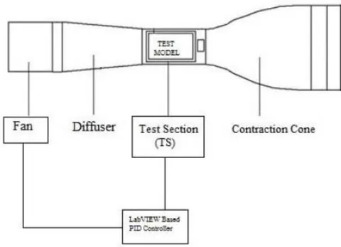
VI. IMPORTANT DEFINITIONS AND MATH INVOLVED

a) Fluid Mechanics Terminology

Fluid Mechanics

Having wide range of applications such as Mechanical, civil, chemical, biomedical, geophysics and astrophysics, Fluid Mechanics is a branch of physics pertaining to fluids-Liquids, Gases and Plasmas. It could be further subdivided as Fluid Statics (Study of fluid at rest) or Fluid dynamics (Study of forces and its effects on motion of fluid) [97]. It a subset of continuum mechanics, a study concerning macroscopic viewpoint of matter. Fluid Mechanics, is notorious in terms of active research.

Fluid Statics

Study of fluids (compressible as well as incompressible) or pressure in/exerted by fluid on immersed bodies, at rest in stable (Hydrostatic) equilibrium is termed as Fluid Statics or Hydrostatics. It gives a plausible reasons for phenomena like change in atmospheric pressure with altitude, water floating in oil and retainment of shape of water in the container. It is the root and lays foundation for Hydraulics. Plate tectonics (Meteorology), Blood pressure (Medicine) and so many other fields are applications for the same [98, 99]. Terms such as Buoyancy, hydrostatic pressure are part of this study.

b) Fluid Dynamics

Another sub-discipline of fluid mechanics pertaining to fluid flow (science of liquids or gases in motion) is called Fluid Dynamics [100]. It follows a systematic approach of utilizing empirical and semi-empirical laws derived from measurement of flow to solve practical issues. These solutions involve calculations of properties such as velocity, pressure, density, and temperature of fluid as functions of Space and time. It lays the foundation for: Aerodynamics-Study of air/gases in motion $[100-104]$ and Hydrodynamics (Study of liquids in motion) $[105-106]$ Calculation of forces and movements on aircraft, estimation of mass flow rate, prediction of weather patterns as well as modelling of explosions could be achieved by Fluid Dynamics.

Flow Types

Laminar Flow

Laminar flow is the passage of fluid in thin parallel layers that roll over one another like paper sheets. Each layer is subjected to heavy viscous forces from neighbouring layers, which dampen flow disturbances, allowing flow downstream of an obstacle to easily return to its original state.

Turbulent Flow

Turbulent flow is a particularly random and turbulent flow characterised by the forming of eddies and vortices of various sizes. It occurs at high Reynolds numbers and is characterised by the formation of eddies and vortices of various sizes. Unlike laminar flow, where viscous forces are the primary determinant of fluid behaviour, turbulent flow is governed by inertial forces. Fluid behaviour in turbulent flow is notoriously difficult to quantify. [47]

Compressible Flow

Fluids and fluid flow that undergo change in density due to change in pressure or temperature are compressible fluids/flows

Incompressible Flow

Fluids and fluid flow, for which changes in density are insignificant when pressure and temperature change are incompressible fluids/flows. In most cases, modelled flow is incompressible. Mathematically when expressed, density not changing as it moves in flow field is represented as:

Where, $\frac{D}{Dt}$ is material derivative (sum of local and convective derivatives)

Steady Flow

A flow which isn't a function of time and whose properties do not alter over time are deemed as steady flows

Transient or Unsteady Flow

Flow dependent on time is called unsteady or transient Flow. Choice of frame of reference depicts whether flow is steady or unsteady.

Newtonian and Non-Newtonian fluids

In a variety of fluids like water or air, where, stresses due to viscous forces are directly proportional (related linearly) to strain rates are called Newtonian Fluids (Shown by Isaac Newton). This coefficient of proportionality is termed as Viscosity of fluid (property independent of strain rate) On the other hand, Non-Newtonian fluids, are much more complex involving non-linear stress-strain behaviour, and include fluids such as blood, polymers, honey and lubricants.

Drag

A constituent of force projected along the direction of motion is called as Drag. Shear forces as well as pressure induce drag for body in motion. Skin friction drag, also known as parasitic or profile drag, is a portion of overall drag encountered by a body in a fluid flow as a result of frictional forces between the fluid and the body's surface. It is more substantial in streamlined entities. Skin friction is the only source of traction where there is no boundary layer separation [47]. Pressure drag on the other hand is noteworthy in case of blunt objects. [19, 14]

The drag force is generally non-dimensionalized as a function of Reynolds, which referred as drag coefficient [19].

The pressure coefficient could be obtained on the same terms, by normalizing dynamic free stream pressure and then rewritten as reduced pressure coefficient. [19]

Boundary Layer

Boundary layers are regions of fluid immediately adjacent to an immersed object or wall, under which flow velocities are controlled by viscous forces. They possess a pivotal role in experiments. The fluid in this area is responsible for the bulk of the drag forces and heat exchange endured by the object. Boundary layers usually start out as a thin laminar flow area that thickens with rising Reynolds numbers and then transforms to a turbulent layer flowing over a viscous sub-layer. Outside of the boundary layer, the flow is unaffected by Reynolds number criteria. Two dimensional boundary layers are suggested to reduce the disparity between theory and tests. [19, 21, 50, 94]

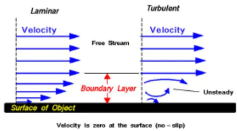
c) Fundamental Equations

The equations of paramount importance derived for modelling Wind tunnels especially low speed ones, are three in number [45, 46]. They are also, the fundamental principles/axioms governing fluid mechanics, (all are based on classical mechanics, modified in quantum mechanics and general relativity wherever, needed). They are expressed via Reynolds Transport theorem generally. The principles are:-

1. Conservation of Mass or Mass Continuity theorem.

2. Conservation of Momentum or Newton's Second Law linking force and motion

3. Conservation of Energy or First Law of Thermodynamics governing energy exchanges

The Conservation laws could possess an integral or a differential form and are applied to regions called as control volumes, which are discrete volumes in space where fluid is estimated to flow. For description of changes in mass or energy within control volumes, integral formulations are implemented, meanwhile, differential formulations apply Stokes Theorem to yield expressions which could be referred as integral forms applied to infinitesimally small volume (at points) within flow.

In addition to these, we utilize definitions of fluid properties, their variations with pressure and temperature (e.g. Gas Law PV=nRT) for added accuracy. Also, fluids are assumed to obey the continuum assumption that they are not discrete, rather continuous, and properties such as velocity, density etc. are well defined at infinitesimally small points varying continuously at different points. Only a brief gist is presented here. To delve into the topic further, readers are suggested to refer to Anderson [95], and Currie [96]. Mass Continuity (Conservation of Mass)

Mass is neither created nor destroyed in a control volume, hence, rate of change of fluid inside control volume is equal to net rate of flow in the volume, itself [107]. It is also referred to as equation of continuity [46, 50]. A differential form of continuity equation, by the help of divergence theorem could be stated as:

Where, $\rho$ is the fluid density, u is the flow velocity vector, and t is time.

For quasi 1-D incompressible (density of fluid constant) flows, it simplifies [47] down to $A_1{V}_1=A_2{V}_2$

Conservation of momentum

Newton's second law of motion applied to a control volume (element of fluid) gives the statement: Changes in momentum of fluid within control volume are caused by net flow of momentum into the volume as well as by the external forces acting on it. This momentum balance is valid for stationery as well as moving control volumes. [46, 107] When volume is curtailed to infinitesimally small point, the differential form is obtained:

ρ is Fluid density

F is Force and consists of both, surface forces (viscous/shear forces) and body forces. It can also be expanded for frictional, electromagnetic or gravitational forces acting at point in flow. [46]

Navier Stokes Equation In aerodynamics, air is believed to be a Newtonian fluid, which implies that the shear stress (due to internal friction forces) and the rate of strain of the fluid are linearly related. The equation above is a three-dimensional vector equation that can also be expressed as three scalar equations in three coordinate directions. The Navier–Stokes equations are the conservation of momentum equations for compressible, viscous flow cases $[107]$ such as, fluids that do not possess ionized species, are sufficiently dense to be in continuum, and retain that velocities to be minor in comparison to speed of light.

Navier Stokes equations (after, Claude-Louis Navier and George Gabriel Stokes) are a non-linear set of differential equations describing flow of a fluid whose value of stress depends pressure and on the flow velocity gradients linearly. They relate pressure, density, temperature, velocity of fluid through use of stress and strain rate tensors and depict the force balance at a given point in fluid [47]. When a body travels through a fluid, forces produced by the fluid's viscosity, inertia, elasticity, and gravity, are explicitly described by the different terms in these equations [Chapter 2, [45]]. For an incompressible fluid with u as the velocity vector, the Navier Stokes equations are: [109-112]

Additionally, at times gravitational or Lorentz forces are added. Which result in set of five coupled differential equations and additional state for solution.

These differential equations are analogous to Newton's equation of motion for particles for deformable materials. Here, momentum (force) change is depicted in contrast to pressure P and Viscosity is parameterized by kinematic viscosity v

The solutions to these equations for any physical problem is usually sought after using calculus, however practically, only simple cases could be solved using them (involving non-turbulent, steady flow, whose Reynolds number is small). For complex cases (ones with turbulence involved [47]), such as aerodynamics, hydrodynamics, global weather systems etc., the solutions could only be found via computers and their aid, as these unsimplified equations do not possess general closed form solutions. This aid, for partly or wholly unsolved practical problems addressed by numerical methods/approximations gave rise to the branch of "Computational Fluid dynamics (CFD)" [47, 113-117]

Note:

Newton's $2^{\text{nd}}$ law helps describing dynamics of fluid particles, however, an accelerating parcel of fluid experiences inertial forces. Reynold's number discussed ahead, a dimensionless quantity characterises flow.

When $R_E$ is low and <<1, viscous forces are predominant rather than inertial forces, and if inertial forces are neglected, the flow is called "Stokes or creeping Flow".

When $R_E$ is high and >>1, inertial forces are predominant and the viscous forces are neglected, thus the flow modelled is called "Inviscid flow"

If the viscosity effects are eliminated from Navier-Stokes Equations, it simplifies to "Euler Equations" When the Reynolds number is high, this strategy can be very effective. However, certain issues, such as those concerning solid boundaries, can necessitate the inclusion of the viscosity. Since the no-slip state creates a thin area of high strain rate. The boundary layer, in which viscosity effects prevail, produce vorticity, viscosity cannot be ignored along solid boundaries. As a result, viscous flow equations must be used to quantify net forces on bodies (such as wings) and the inviscid flow theory struggles to simulate drag forces, a drawback known as the d'Alembert paradox.

A widely used model in computational fluid dynamics is infact the use of 2 flow models: the Euler equations away from the body, and boundary layer equations in a region close to the body. The two solutions could be then compared with each other, using the method of matched asymptotic expansions.

Conservation of energy

The total energy will always remain constant, even though it could convert from one form to other. The expression could be given as:

Here, the left side expression is a material derivative where, h is the specific enthalpy, k is thermal conductivity of fluid, T is temperature and phi is the viscous dissipation function governing the rate of conversion of mechanical energy to heat. It is generally positive, that is viscosity cannot create energy within control volume. [108]

Another way of stating this law would be: Change in total energy comprising of internal and kinetic energy is nothing but the sum of total work done on system and energy transferred by thermal conduction [46].

Bernoulli's Principle

A huge pivotal principle is fluid dynamics is the Bernoulli principle, stating that "Increase in speed of fluid occurs simultaneously with decrease in static pressure or decrease of fluid's potential energy" (named after Daniel Bernoulli, publishing it in his book "Hydrodynamica" in 1738). Euler also, put forward paramount Bernoulli equation confirming deductions of pressure decrement when flow speed is increased.

It is applicable for isentropic flows (enthalpy constant) where irreversibility, and non-adiabatic processes are neglected. This principle has many forms as it could be applied to various flows resulting in different form. The basic form (stated here below) is the Bernoulli principle for incompressible flow. Higher advanced forms applicable to compressible, unsteady flows are not presented in this study.

Bernoulli's principle could be derived from either Principle of Conservation of energy or from Newton's second law of motion. (Both stated above). In terms of conservation of energy it states "For steady flow, sum of all forms of energy in a fluid along a streamline is at all points along that streamline", whereas, in terms of the $2^{\text{nd}}$ law of Newton (conservation of momentum), "There is more pressure behind rather than in front when a small volume of fluid flows horizontally from region of high pressure to low pressure, giving rise to net force on volume, which accelerates it along the streamline".

It represents a relation between velocity, density and pressure [50]. The equations assume incompressible (constant density), steady and inviscid (viscosity negligible) flow) flow and could be given by:

Where, g is acceleration due to gravity, Z is elevation of fluid from arbitrary datum, P is Pressure (static pressure), $\rho$ is fluid density, and u is velocity. [18, 45, 46]

The term $\frac{1}{2}\rho u^2$ is referred to as dynamic pressure (also called velocity pressure by authors), and expresses fluid's kinetic energy per unit volume

The term $\rho gZ$ is the gravitational potential energy of the fluid

The end term P is the static pressure, or a measure of internal energy of the system

Sometimes a term $h=Z+\frac{P}{\rho g}$ is also used, which stands for Hydraulic Head or Piezometric head.

For many practical applications like flight of aircrafts and wind tunnels, the gravitational potential energy term is minor as compared to the other two, as change in height is minimal, and if neglected, gives the equation for Stagnation pressure:

Total pressure = Static pressure + dynamic pressure

Note: The stagnation pressure of a system is constant under the same set of assumptions, however, in practice, for non-ideal systems like wind tunnel, viscous forces are not negligible throughout. Hence, inefficiencies in the Wind tunnel can be expressed as drops in stagnation pressure. This could aid the fundamental design process.

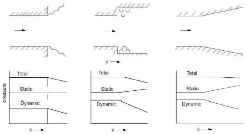
d) Important Testing Parameters and Scaling of Models in Wind tunnel

The test models or probes need to be scaled down to fit the dimensions of the wind tunnel's testing section. When scaled down, apart from just geometrical similarity, there are certain parameters that must retain themselves which are pivotal for aerodynamic calculations of the model and important for obtaining the same wind flows around the model at its actual true full scale. These parameters are Reynold's Number (For low speed Wind Tunnels), Mach number (For Medium Speed Wind Tunnels), and Froude Number (For High Speed Wind Tunnels) formed by relating various forces to inertia force (some are excerpts from non-dimensional Navier stokes equations as well.)

Reynolds Number

It is a chief parameter used by engineers to estimate the flow whether it is laminar (smooth flow free from eddies) or turbulent (consisting eddies and randomness). Implementing the dimensionless forms of Navier Stokes equations, Reynold's number is determined as the ratio of inertial forces to the viscous forces (with no dimensions). [10, 47]

Using the mean velocity (u), Characteristic diameter/length ( $L_{char}$ ), density( $\mu$ ) and viscosity, valid for any fluid, Reynold's number could be calculated as:

It is dependent on geometry of section, roughness of the walls. [19]

Osbourne Reynolds had identified this parameter in 1883. A common distinction found is: If , flow is laminar, , flow is turbulent, and otherwise it is in transit. [19, 47]

Reynolds number is a vital and primary similarity parameter for low-speed wind tunnels with M < 0.3 [Chapter one, [45]] [10]

Mach number

It is of paramount importance for flows occurring at high velocities which cause variation of density and temperature of fluid. Speed of an object traversing through air or any other fluid divided by the speed of sound gives, "Mach number", a dimensionless quantity. [47, 50, 52]

It is generally used for representing speeds of object close or above speed of sound. It is affected by the composition of medium surrounding it, and also, by the local conditions such as temperature and pressure. Mach number is used to detect whether flow is Incompressible or not. Incompressibility is a good assumption for certain liquids, but in case of acoustic studies, soundwaves is considered compressible.

Froude Number

This number plays an effective role when gravity forces are involved, reason why, they are used for model drop tests. It helps simulate supersonic waves as well [19].

It is defined as:

Froude Number is good for flows which have free surfaces and it is an important similarity parameter only if there exists unsteady boundary conditions, or for dynamic systems such as towed bodies. [Chapter one, [45]] Froude number is absent when fluid body forces are ignored, which is a common assumption for most of the fluid flows.

Note: Prandtl number- Not in consideration in this study, as it appears only in cases of heat conduction. It is ratio of viscous diffusion rate to thermal diffusion rate.

Scaling Principles

The requirements for big models to be scaled down to be placed inside wind tunnels are:

Geometric Similarity

The geometric similarity between the model and the prototype is one of the most significant considerations for models. By geometric similarity, we say that the model and prototype should have the same ratios of corresponding dimensions (scalability). [23]

Dynamic Similarity

The dynamic similarity theorem states that a scale model with the same similarity parameters such as Reynolds number and Mach number would have forces and moments that can be directly scaled. The full-scale body and the model would have identical flow patterns $[19,23]$

In reality, matching both Reynolds number and Mach number to full scale in a model experiment is rare. In truth, there are times when neither the Reynolds number nor the Mach number can be balanced. After that, decisions must be taken based on the parameter is considered to be the most relevant for the type of flow situation in question. Mach number matching is normally only applied to flight vehicles in the high-speed flight area, where Mach number effects predominate and Reynolds number effects are less significant. In low-speed flight, Reynolds number effects predominate, and Mach number matching is less important. However, every experiment should provide a thorough examination of the impact of Reynolds and Mach numbers to ensure that the effects can be generalised to the full-scale problem. [45]

This principle is used in other engineering fields as well, giving numbers such as: Stanton Number (St, ratio of heat transferred into fluid to thermal capacity), Strouhal number for experiments with oscillating flow, Knudsen number ( $K_n$ ) for low density flows, Euler number, Eckert number etc. [49, 23]

Note: If scaling is successful, the non-dimensional functions for fluid velocity components, pressure coefficient, density, viscosity, and temperature would be the same. As a result, the force and moment coefficients for the model and full-scale flows would also be similar. Chapter 2 of [45] states

"Under these conditions, the forces developed by the model can be directly related to the forces on the full-scale article by multiplying the force coefficients obtained in the experiment using the model by the factor $\frac{1}{2}p{v}^2{L}^2$ with the values of parameters in the factor corresponding to full scale." And "the moments developed by the model can be directly related to the moments on the full-scale article by multiplying the moment coefficients obtained in the experiment using the model by the factor $\frac{1}{2}p{v}^2{L}^3$ with the values in the factor corresponding to full scale."

E.g. To improve design of golf ball- If a golf ball has a diameter of 0.04 metres and travels at 25 metres per second in air at sea level, it has a Reynolds number of 68,200 and a Mach number of 0.06. As long as the Reynolds number is the same, you can make a big model, say 0.2 in diameter, and test it in your wind tunnel. Since there is no noticeable compressibility effect, the Mach number may be overlooked. To meet Reynolds number, you'd have to use a wind tunnel with a free stream velocity of 5m/s. The golf ball's boundary layer and the wake behind it will be perfectly scaled under these conditions. If the golf ball in flight has a 0.001 metre thick boundary layer at one point, the model's equivalent point would have a 0.005 metre thick boundary layer.

VII. CFD INVOLVED AND TURBULENCE MODELS

CFD standing for Computational Fluid Dynamics, tries to solve differential equations governing fluid flow using approximation of numerical means. It had been use first with respect to performance enhancements for wind turbines with 2D aerofoil properties, but now is employed at all scales: Airfoil to atmospheric boundary layers. CFD has been termed as "Multiscale virtual wind tunnel" due to its vivid applications and as it provides deeper insights [2]. It helps in exploration of shape, and character of fluid flow. It simulates closer to real conditions flows, as well as curtails the errors via tolerances. Variety of parameters such as velocity, turbulence intensity, distribution of fluid flow, pressure distribution could be obtained via CFD [3].

Despite numerous advantages, there are limitations imposed by CFD in terms development and application of a mathematical model to simulate the results of turbulence known as turbulence modelling (eg. Real life scenarios, including the flow of blood through the cardiovascular system, the airflow over an aircraft wing, the re-entry of space vehicles etc.). As mentioned above, exact solutions of turbulent flows is extremely difficult and complex, especially for high Reynolds number. Modelling turbulent flows is an impediment for fluid mechanics $[45]$. Regardless of decades of study, there is no analytical hypothesis that can determine how these chaotic flows will evolve. CFD simulations use turbulent models to simulate the evolution of turbulence in most real-world turbulent flows. This turbulence models are simplistic constitutive equations that forecast turbulent flow statistical evolution. Treatment of transition to turbulence and roughness implications are critical topics that the scientific community are currently addressing.

a) The Closure issue

The Navier Stokes equation described above, governs velocity and pressure of fluid flow, which could be split into a mean and fluctuating components for a turbulent flow giving rise to "Reynolds-averaged Navier Stokes (RANS) equations". Due to non-linearity of Navier stokes equations, the velocity fluctuations still appear in RANS equations in the non-linear form $-\rho \overline{u_i^{\prime }{u}_j^{\prime }}$ from convective accelerations, which is termed as Reynolds Stress $R_{ij}$. It effects the mean flow in the same way as stresses like pressure or viscosity. By removing reference to fluctuating parts of velocity, closure of RANS equations by modelling of $R_{ij}$ as function of mean flow, is needed to obtain equations containing only mean velocity and pressure, which is the "Closure problem".

b) Eddy Viscosity Models

The first to delve into closure issue was "Joseph Boussinesq" who introduced the "Eddy Viscosity" concept, relating stresses of turbulence to mean flow in order to close the system of equations. The models are coined as "Eddy viscosity models" (EVMs) [121].

This Boussinesq hypothesis brought about a variety of turbulence models offering lost computation costs which help replicate right flow conditions, such as the "Spalart-Allmaras" (S-A), "k-ε" (K-epsilon), and "k-ω" (k-omega). S-A utilizes only one additional equation to model the turbulence viscosity transport while, the other two use two additional equations. A brief overview of these models:

Spalart-Allmaras (S-A)

A one equation model solving the modelled transport equation for kinematic eddy turbulent viscosity, employed for applications of aerospace (wall-bounded flows) is the S-A turbulent model $[122]$. It provides nice results for boundary layers subjected to adverse pressure gradients and is popular amongst, turbomachinery applications.

$k-\epsilon$ (K-epsilon)

One of the most common CFD turbulent model, used to simulate mean flow characteristics for turbulent flows and possessing 2 equations to provide general description of turbulence by means of transport equations (PDEs)[123]. First thought for K-epsilon was for improving mixing length models and finding an alternative to algebraic of turbulent length scale in moderate or complex flows. It is proposed and is robust enough to predict airflow away from wall/surface and calculates factor turbulence kinetic energy 'k' (energy transport) and dissipation energy (rate) 'ε' using Boussinesq hypothesis. [2, 3]

$k-\omega$ (K-omega)

Another common two-equation turbulence model used to solve closure issue. It tries to predict turbulence using 2 partial differentials for 2 variables: k (turbulence kinetic energy) and $\omega$ (specific rate of dissipation of k into internal thermal energy and $\omega \approx \epsilon /k$ ) [3, 124]. It possess the ability for predicting airflow nearer to wall or surface, and calculating freestream value, moreover, offers accuracy in predicting free shear flows. [3]

SST (Shear Stress transport)

Menter's Shear stress turbulence model is commonly employed robust 2 equation model used in CFD. It combines both k-ε and k-ω models in such an efficient way that the k-omega implemented in the inner region of boundary layer switches to k-epsilon in free shear flow. [125]

Large Eddy Viscosity Model

It is analogous to DNS (Direct numerical solutions) with high $R_E$ (Reynold's number). It uses a filter that passes through a small turbulence energy to the average and model a flow, a method known as "subgrid scale modelling". The hurdles in applying LES (Large eddy viscosity) to wall-bounded flows, mainly caused by impractical grid requirements in the near-wall region. [2, 3]

c) Reynolds Stress equation model (RSM)

Referred to as $2^{\text{nd}}$ moment closure model, RSM model is one of the most complete classical turbulence model approach. While the above 4 utilize eddy viscosity equations, RSM implements Reynolds Stress transport equation. The drawbacks of k-epsilon and k-omega such as flows with anisotropy, streamline curvatures, flow separations, and recirculating flow zones influenced by rotational effects are overcome by RSM models offering much better accuracy. [3, 126-128]. Also, in regions where turbulent flow behave like elastic mediums predominant in eddy viscosity closure's rapid distortion limit, RSM is much more helpful [129, 130]. The basic concept is similar to other models mentioned above but RSM could help calculate pressure strains of each unit in all directions (by partially resolving it) which is generally reasonable for asymmetric turbulence phenomena. [3]

d) Measurement using CFD

Turbulence Kinetic Energy, as well as Flow velocity are most common strictures to estimate performance of the Wind tunnels. [49] These parameters could be found from both CFD (Computational fluid dynamics) as well as experimental results.

In some papers like $[8]$, a CFD code is applied for calculations of 3 dimensional RANS as well as continuity equations, which utilizes control volume method alongside Semi-implicit Method for Pressure-Linked Equations (SIMPLEC) velocity pressure coupling algorithms with $2^{nd}$ order upwind discretisation. Performed on basis of standard k-epsilon model. Another one [3], uses commercial ANSYS FLUENT release 15, and the same SIMPLEC algorithms.

VIII. OUR DESIGN AND ANALYSIS

From Literature review and analysis of all wind tunnel data, we get the below "Table of Design".

a) Procedure or Plan of action implemented

1. Research and delving into the topic

2. Literature review and accumulation of design data about a variety of Wind tunnels

3. Arranging of data

4. Shortlisting of design according to guidelines, strictures and constraints

5. Design modelling in Autodesk Fusion 360.

6. Choosing a single design as basic design

7. Creation of assembly of the same design in Autodesk Inventor

8. Import of model in Autodesk CFD

9. Study A:- Keeping basic set of assumptions and constant boundary conditions, different turbulent models are deployed, (k-ε, k-ω, SST k-ω and LES) on:

a. Plywood as material of components, while test section as glass b. Plywood as material of components, while test section as acrylic

c. Aluminium as material of components, while test section as glass d. Aluminium as material of components, while test section as acrylic

10. On basis of conclusions obtained, choosing the material and right turbulent model to be constant for next set of testing.

11. Study B:-With fixed material and turbulent model, and again, keeping the basic set of assumptions and boundary conditions fixed, this time different geometries are used-

a. Circular diffuser b. Octagonal contraction cone

c. Contraction Cone with different polynomial of wall curve

12. Study C:-With the previous optimized model, different scenarios are used.

d. Increased length of settling chamber e. Thickness is varied

f. Test section length reduced.

13. Comparisons are made with our basic square cross section contraction and diffusers and inferences are made

14. Final Design is created in Autodesk Fusion 360

b) Preliminary data collection

First a number of Wind Tunnels were analysed and their data were arranged in various tables using MS Excel. The variety of tunnels were of different types, dimensions and speeds.

Figure 23: Table of Design Data

A. NO.

PAPER

OPEN OR

TOTAL

VELOCITY

CONTRACTION

CONTROL TABLE

CONTROL FROM CONTRACTION

TEST SECTION

SHAPE OF

DIFFUSER

DIFFUSER

DIFFUSER

ADDITIONAL

ANY FACULTY

TEST

DETAILS OF

FAN

1

OF RESEARCH

CLOSED

LENGTH

(in mm)

RATIO (USQUALLY IS TO 1)

LENGTH

SEM ON FILL-IN DEGREE

(0,8 ft)

TEST SECTION

LENGTH

ANGLES

COMMENTS

MATERIAL

HC AND SCREENS

SPEC5

Computer Control wind tunnel

6.6m

0.1mm

2

2.7m

20-12.4" 12" 5m

Rectangle

30-6 ft" 17 m

square

A and Turbine Study of Wind Loans and model wind turbine at atmospheric boundary layer walls

(20-2.4" 2.5" 0.99)

rectangle

A. Asequeable design and characterization of the 2D printing, a specific wind tunnel of the 2D pipe

VERTICAL OPEN AND LABORATION

20/4km

15, 15 to 42

3.83m

(0.4" 4.3" 2m

Rectangle

Dimensions closed

0.4" FD 70.12" one of the 5 dimensions given in table

PITOT-HISA ARRANGEMENT, setting chamber - (0.4" 4.3" 5m)

DELPT

The flow straightener is custom made using completed stainless steel of 0.127 mm thickness. The horizontal cell size is 0.5 mm. The open area coefficient is approximately 94%. The streamwise length of the flow straightener is 140 mm

A. Anystylytic design in cycling patterns. New height by CPD simulation and wind tunnel

2.1" 15 m

The maximum thickness ratio is 0.8%, which is well below the maximum maximum value of 27% (Piping et al., 2007-Tennagga et al., 2008).

Wind Tunnel Laboratory at the University of Large in Belgium

Analysis of subscale wind tunnel with variation of shape rectangular and polygonal on site

LAREMAR

1.35m

28m

5 variations

0.9" 0.9" 2

5 variations

a modified translocus, set turnee for NASA 2012

Aerosynthetic boundary layer modeling: on site wind tunnel

CLOSED

15

(1.9)" 0.6" 6m OR 3°/7.9" 6m)

square

0.6m

The Reversible Augmented Nanom-Skiss apparatus was added by second order little volatility method based on the SST two mode and the velocity and substance intensity were measured by double displacement.

A modal wind tunnel for sound wave field measurements

1.5m

1.5"x20.7x 6m (bit)

CFO in Wind/Electro The Wind/L Mechanical Wind Tunnel

TURB

Here, a two-sided tested and tapered rotor was located in the NASA Research Center 24.4 x 36.6 x Wind Tunnel.

Computational Test dynamics simulation of the tolerance module in the tested section on wind tunnel

OPEN

5.628

The airflow is assumed friction absence because the test chamber material is from acyclic, in triple of fine, the flow is chosen to serve in three dimensions, and the flow is used as a minimum of 1.24m.

square with curved radius 0.250

Unshared the force is located after the diffusion (Thermal Hardness of Air Quality) of 1.25°C, while a maximum force of 0.75 m/s.

CONSTRUCTION DESIGN FOR SHALL LOW SPEED WIND TOLERANCE AND RESTRICT AND BREADWATER

After testing-completion is a safety of design, it has found for the entire assembly 0.1, 1, 1, or we represses use 0.18m on above the line

1m-wide -86m

100-100 feet width is a run-rate of 100m and two run-rate cut-off of 10m that about 40 m.

arcass of arcass of arcass of arcass of arcass of arcass of arcass of arcass of arcass of arcass of arcass of arcass of arcass of arcass of arcass of arcass of arcass of arcass of arcass of arcass of arcass of arcass of arcass of arcass of arcass of arcass of arcass of arcass of arcass of arcass of arcass of arcass of arcass of arcass of arcas.

arcass of arcass of arcass of arcass of arcass of arcass of arcass of arcass of arcass of arcass of arcass of arcass of arcass of arcass of arcass of arcass of arcass of arcass of arcass of arcass of arcass of arcass of arcass of arcass of arcass of arcass of arcass of arcass of arcass of arcass of arcass of arcass of arcass.

A and designed diffusion an extending junction with a constant degree of about 1.4 m tilt angles (opters)

1. The solid guidelines followed by design by cycle an arc as a minimum of 1.0 m tilt angle and the roll-off of corresponding frame at the same and compared to the side and 2.750 OBOOD POLITICAL CHS

5 CONTRACTOR DESIGNER GRIEDS

Design and fabrication of low speed wind tunnel and flow analysis

OPEN

30 m and 40 m

4

1.5m

24

(0.75" 0.5)m

square (The test section was made with the help of physics and floor glass. The maximum thickness range of 2.5 cm) was added to the left side of the test section was fabricated with the right surface.

Outer 0.7m, inner 0.5m

1.6m

7

sitting chamber - (0.7" 1)m

Corporated Specification Motor power 7-1 HP. Maximum Speed of one 1400 rpm Type of motor 3-phase induction motor

Design and performance of a small scale aromatic solvent tunnel

CLOSED

UPTO 80 M/S

9

1m*1m

CLOSED AND OPEN TEST SECTION FOR APROGRAVATE AND AEROACUCOSTIC RESPECTIVELY

The DS asequeac wind tunnel at Bulking University is a newly commissioned small-scale crosscellratic wind tunnel with low fluidance intensity and low background noise.

Design and performance of a small scale wind tunnel for building research

OPEN

0.25 fm

209

(8°20' 0.9"(K/L)

rectangle

Design methodology for quick and low cost wind tunnel

CLOSED, TURBLOWER CONTINUING FLOW

2 SEGMENTS OF 3ND DEG POLY CURVE

80 m x 4 TO 6, RECOM/3

80m x 4 TO 6, RECOM/3

BOTH-CONTRA SEM ANGLES IN ORDER OF 12

1"

Rectangle

3.5

three-dimensional tests, a typical with to height ratio is 4.3; lenses, for tachedralness ratio is 2.5 and a ratio is added in order for the boundary layer thickness in the test section be much similar than the model space.

The one on the site is located in the Technological Centre of the LPM-MAle (Markel) and test chamber sections 1.20 x 1.00 kΩ, the system application is mainly research. The right is located in the Bupleura Laboratory of the Astracuate School of the LPM- will test chamber sections is 2.80 x 1.20 m2.

a 2.0m diameter fan specialty designed for this purpose or commercial fan of 1.0 m diameter.

Design of an open-circuit substore wind tunnel for educational purpose

OPEN

4.5m

20-25 m

6.25

1m

(0.75" 0.4)m

square

2.405

1.8m

6 TO 7

FULL SPECIES GIVEN

Design optimization of three dimensional parametry of end-to-end connection

OPEN-JET BLOWER TYPE WITH2 BLOOMERS WITH2 DIFFUSERS

Inner 120m

The old construction has a square cross section of 100-150 cm2 at 80-80 cm2 and a contraction ratio (CR) of 3.5 ft above the lower the recommended contraction ratio (0.5). The optimal contraction has an end cross section of 80-80 cm2 and a contraction ratio of 2.5 cm2 at 150 cm2 on the next section of the recommended ratio of only between length and hydraulic diameter at the construction grid

The first diffuser separation from 30-50 cm to 50-100 cm over a length of 120 cm, giving a maximum edge of 21.6 and an area of 107. The second diffuser separation from 50-100 cm to 74-150 cm over a length of 100 cm, giving a maximum edge of 20 and an area of 3 cm.

3rd-order accurate is used for spatial discretization. Shear Swiss Transport (SDT - 3 omega) model is used for satisfaction modeling.

Design rules for small low speed wind tunnel

OPEN AND CLOSED, SINGLE BLOWER AND DIFF

diffuser included angle usually not exceeding "for best flow diseases, although best pressure recovery is achieved at about 107" and an area ratio not exceeding about 2.4. It is important to have a reasonable degree of flow diseases in the first diffuser, since otherwise the pressure recovery tends to fluctuate with time, and, therefore, as close the lateral speed if the first power is nearly constant.

Design, Fabrication and Characterization of Low Speed Open/ Wind Tunnel

OPEN SINGLE BLOWER WITH BLOOM AND DIFF

2 TO 25 m

The contraction has a square intersection of 140×140 cm at a single wire, 5×40×6 cm and a net wire, and a contraction ratio (CR) of 7.85 x 1.04 a length of 140 cm.

The first diffuser part spreads from 50×60 cm2 to 11×10 cm2 over a length of 50 cm, and an area ratio of 1.80. The second diffuser part spreads from 11×10 cm2 to 140×140 cm and a second length of 50 cm, giving a maximum degree of 23.4 and an area ratio of 1.65.

Two sensors with a proximity of 0.67 are placed in the middle between the two sensors.

A Woodhook Lot centrifuge with backboard facing dryng-type blades with a 0.5-1.00 kg of 1.5-3.5 kg electric motor can drive the operation and turnout. The can flacer a wide section of up to 6.0-8.5 cm again static pressure up to 550 Pa.

Design, Manufacturing and Testing of Open-circuit Substrate Wind Turkeys - A Comprehension Review

cell of honeycomb of length 5.10 times the diameter depositing the lateral disturbance of the wind.

cell of honeycomb of length 5.10 times the diameter depositing the lateral disturbance of the wind.

cell of honeycomb of length 5.10 times the diameter depositing the lateral disturbance of the wind.

Cell of honeycomb of length 5.10 times the diameter depositing the lateral disturbance of the wind.

cell of honeycomb of length 5.10 times the diameter depositing the lateral disturbance of the wind.

cell of honeycomb of length 5.10 times the diameter depositing, the diameter depositing the lateral disturbance of the wind.

cell of honeycomb of length 5.10 times the diameter depositing the lateral disturbance of the wind.

cell of honeycomb of length 5.10 times the diameter depositing the lateral disturbance of the wind.

cell of honeycomb of length 5.10 times the diameter depositing the lateral disturbance of the wind.

cell of honeycomb of length 5.10 times the diameter depositing the lateral disturbance of the wind.

cell of honeycomb of length 5.10 times the diameter depositsing the lateral disturbance of the wind.

cell of honeycomb of length 5.10 times the diameter depositsing the lateral disturbance of the wind.

cell of honeycomb of length 5.10 times the diameter depositsing the lateral disturbance of the wind.

40 m

8

A test section of square cross-section of 0.3 m wide at an air velocity of 40 hrs was selected. The test chamber has to live in the range of 0.5-3 times the hydraulic diameter. The length of the test section was set to 1.3 times the hydraulic diameter of the test section, is 1.25m

The test section, which may be closed, open, partially open or convertible, then section length to hydrahy diameter may typically be the channel. The maximum section has a 11% associated correspondence to the front side of the test model. A distance of at least three foot section length. The point of fixed section equal to the range of 2.5 cm, with the well connected to having more doxide. The area ratio to a typical 2.5, again with the smaller volume having more doxide. (BURCL29 [28, AND POPS])

The best flow diseases can be achieved by keeping the diffuser angle at about 30. The length of the diffuser depends on the variable. The final variable is the diameter and cross-section area of the test section and the second variable is the area ratio above 100% of the diffuser. The detailed AR of the diffuser should be around 3.6% keeping the specified core angle of 30. The elongation half angle of the diffuser ends should be less than 3.0% for critical details. The optimum diffuser included angle to achieve flow diseases in the first diffuser, since otherwise the pressure recovery is achieved at about 100 and the area ratio should be between 2 to 3.4

cell of honeycomb of length 5.10 times the diameter depositing the lateral disturbance of the wind.

cell of honeycomb of length 5.10 times the diameter depositing the lateral disturbance of the wind.

cell of honeycomb of length 5.10 times the diameter depositing the lateral disturbance of the wind.

cell of honeycomb of length 5.10 times the diameter depositing the lateral disturbance of the wind.

cell of honeycomb of length 5.10 times that allows for a minimum of 10 ms by removing an effective position of an external fan.

cell of honeycomb of length 5.10 times that allows for a minimum of 10 ms by removing an effective position of an external fan.

cell of honeycomb of length 5.10 times that allows for a minimum of 10 ms by removing an effective position of a external fan.

cell of honeycomb of length 5.10 times that allows for a minimum of 10 ms by removing an effective position of a external fan.

cell of honeycomb of length 5.10 times that allows for a minimum of 10 ms by removing an effective positions of a external fan.

cell of honeycomb of length 5.10 times that allows for a minimum of 10 ms by removing an effective positions of a external fan.

cell of honeycomb of length 5.10 times that allows for a minimum of 10 ms by removing a effective positions of a external fan.

cell of honeycomb of length 5.10 times that allows for a minimum of 10 ms by removing an effective positions of a external fan.

cell of honeycomb of length 5.10 times that allows for a minimum of 10 ms but does not require an effective position of a external fan.

cell of honeycomb of length 5.10 times that allows for a minimum of 10 ms by removing an effective positions of a external fan.

cell of honeycomb of length 5.10 times that allows for a minimum of 10ms by removing an effective positions of a external fan.

cell of honeycomb of length 5.10 times that allows for a minimum of 10ms by removing an effective positions of a external fan.

cell of honeycomb of length 5.10 times that allows for a minimum of 2.5ms by removing an effective positions of a external fan.

cell of honeycomb of length 5.10 times that allows for a minimum of 2.5ms by removing an effective positions of a external fan.

cell of honeycomb of length 5.10 times that allows for a minimum at 2.5ms by removing an effective positions of a external fan.

cell of honeycomb of length 5.10 times that allows for a minimum at 2.5ms by removing an effective positions of a external fan.

cell of honeycomb of length 5.10 times that enables for a minimum of 2.5ms by removing an effective positions of a external fan.

cell of honeycomb of length 5.10 times that enables for a minimum at 2.5ms by removing an effective positions of a external fan.

cell of honeycomb of length 5.10 times that enables for a minimum at 2.5ms by removing an effective positions of a external fan.

cell of honeycomb of length 5.10 times that allows for a minimum at 2.5ms by removing an effective positions of a external fan.

cell of honeycomb of length 5.20 times that allows for a minimum at 2.5ms by removing an effective positions of a external fan.

cell of honeycomb of length 5.20 times that allows for a minimum at 2.5ms by removing an effective positions of a external fan.

cell of honeycomb of lengths 5.20 times that allows for a minimum at 2.5ms by removing an effective positions of a external fan.

cell of honeycomb of lengths 5.20 times that allows for a minimum at 2.5ms by removing an effective positions of a external fan.

celluloclasts of 300 km by removing an effective position of a external fan.

c) Data segregation

The Wind tunnels which matched the description of tunnels we wanted, mentioned above: "Open Circuit (Eiffel) Type Wind Tunnel with closed test sections and with a suck-down apparatus diffuser and fan" were shortlisted. The list was very short, with only a handful of them. They laid the foundation for design in software such as the Autodesk Fusion 360. (Chosen for collaboration, and ease of handling, constructing and modelling data)

Thus, the table of shortlisted designs is given below

SHORTLISTED DESIGNS Figure 24: Table of Shortlisted designs

SR

PAPER

OPEN ORCLOSED

TOTALLENGTH

VELOCITY(in m/s)

CONTRACTIONRATIO (USUALLY IS TO 1)

CONTRACTIONLENGTH

CONTRACTION ANGLESSEMI OR FULLIN DEGREE

TESTSECTION(L,B,H)

SHAPE OFTESTSECTION

DIFFUSER

DIFFUSERLENGTH

DIFFUSERANGLES

ADDITIONALCOMMENTS

ANY FACILITY

TESTMATERIAL

DETAILS OFHC AND SCREENS

FANSPECS

no

10

Design of anopen circuitsubsonic windtunnel fureducationalpurpose

OPEN

4.5m

20-25 m/s

6.25

1m

(0.7*0.4*0.4)m

square

2.405

1.0m

6 TO 7

FULL SPECS GIVEN

13

Design andfabrication of lowspeed windtunnel and flowanalysis

OPEN

38 m/s anduniformpressure 38bar

4

1.18m

24

(0.7*0.6*0.6)m

square

Outer 0.7m,Inner 0.5m

1.6m

7

settling chamber-(0.3*1*1)m

The test section wasmade with the help ofplywood and fiber glass.The manufacturing oftest section top andbottom surface of thetest section wasfabricated of plywoodand side surface wasfabricated with the filerglass.

Component SpecificationMotor power 7.5 HPMaximum Speed of motor 1440 rpmTypes of motor 3 phase induction motorTypes of fan Axial fanfan diameter 1000

WEBSITE

OPEN

8FT

7

2%

1"1"2 (w*1*L)

Square

40

Plywood and Flexiglass

Notice that the fan is circular, but the end is a square, andthat the corners of the board are actually walls that will disturbthe airflow. This can cause turbulence in the Diffuser andaffect the airflow in the rest of the wind tunnel. However, yourfan will negate almost all of this turbulence by drawing thecomor air to the circle and blowing it out.

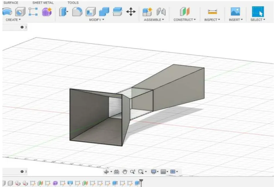
2. Design 2

Model drawn using principles of [21]

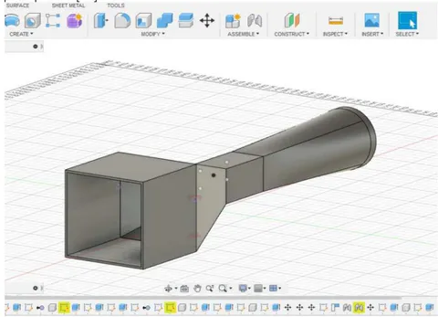
3. Design 3

A little tweaking and using the basic principles from [131].

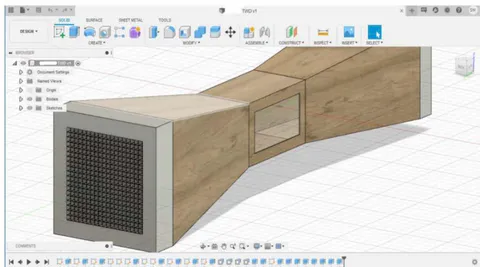
e) Choosing a Base Foundation

The Wind tunnel mentioned in $[131]$, that is after little modifications the design 3 mentioned above, surpassed our expectations and was chosen as a base design. It matched most of the guidelines of design principles mentioned above.

f) Creation of assembly or Model Preparation

This Open circuit wind tunnel was then built in Autodesk Inventor (Implemented for modelling and assembling which is then used as basis for Autodesk CFD analysis later). Separate parts of wind tunnel such as settling chamber, contraction, test section and

Note

diffuser were constructed with a thickness of 0.25 inch and proper scale was employed. The mating with constraints was carried out and the assembly was thus, generated.

In this tunnel, the Settling chamber (consisting of Honeycomb Mesh and Screens) was neglected. This neglecting step was implemented only after failure/error occurring during design study analysis in Autodesk CFD with the screen not responding and the CPU requiring a lot time and processing resources to produce any suitable result for use.

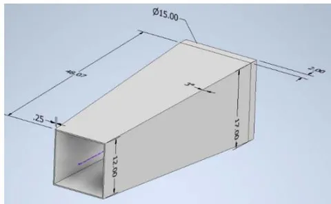
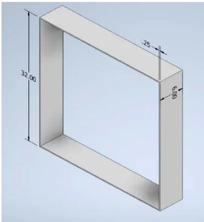
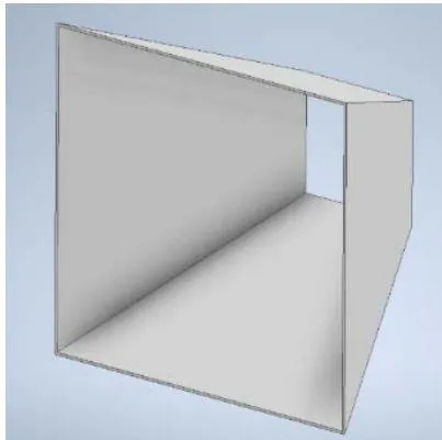
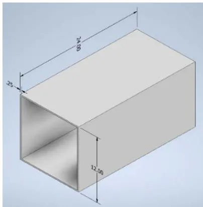
Model in Inventor after assembly:

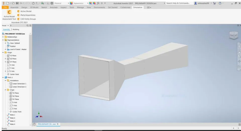
g) Import of Model

Thus, in the following step, this assembly from Inventor is imported to Autodesk CFD for analysis. This software allowed the materials to be set, the control volumes and surfaces to be generated, boundary conditions to be implemented, Meshing to decide, generation of results after solving and reports.

Example of a model in Autodesk CFD-

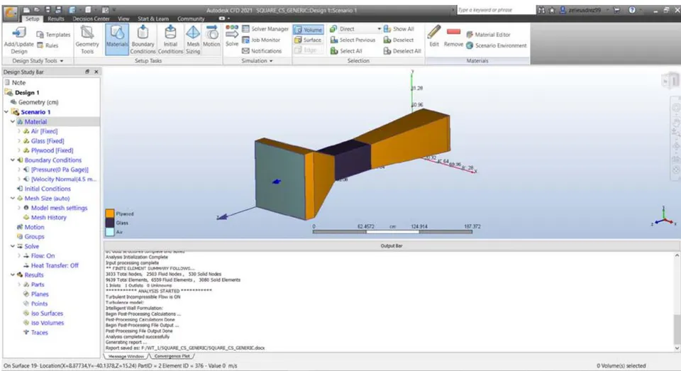
On Surface 19- Location(X=8.87734,Y=-40.1378,Z=15.24) PartID = 2 Element ID = 376 - Value 0 m/s

Figure 33: Plywood components and Glass test section

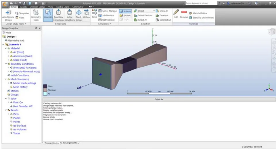
h) Boundary conditions and assumptions

For every model, a few conditions always remained the same:

1. Wind blowing in the Z-direction, since the tunnel runs in X-Y plane

2. Velocity to be normal and of the magnitude 4.5 m/s at the inlet of the cross section or control volume. This value of velocity is used in particular, because, after application of Bernoulli's equations we get decentfan speed capped at 14 or 15 m/s (most fans have speed in these ranges or CFMs of magnitude 7000+)

3. Pressure for the outlet being 0 (static pressure zero, as outlet is open to atmosphere). [1, 21]

4. Control Volume or fluid used is air at standard conditions. (78% Nitrogen, 21% Oxygen, traces of $H_{2}O$, $C{O}_2$ ), below is table for air at STP in imperial and metric units.

Air at "Standard" Condition

Temperature, T	59°F = 518.67°R = 15°C = 288.16°K
Density, p	0.002378 slug/ft ${}^3$	1.225 kg/m ${}^3$
Pressure, p	2116 lb/ft ${}^2$	101,325 Pa (N/m ${}^2$ )
Viscosity, μ	3.74 × 10 ${}^{-7}$ lb-sec/ft ${}^2$	1.791 × 10 ${}^{-6}$ kg/m-s
Kinematic viscosity, ν	1.55 × 10 ${}^{-4}$ ft ${}^2$ /sec	1.44 × 10 ${}^{-5}$ m ${}^2$ /s
Reciprocal of ν	6452 sec/ft ${}^2$	69,440 s/m ${}^2$
Gas constant, R	1714.9 ft-lb/slug-°R	287 N-m/kg-°K
	Imperial	Metric

5. Meshing used is automatic. To keep the study simple and to not change the meshing dimensions each time after importing model, we choose Automatic Meshing. This generates mesh of a particular size, automatically with adequate grid refinement. Moreover, there exists a minimal amount of symmetry within the tunnel. For more processing power, and accurate results one could use unstructured meshing [3].

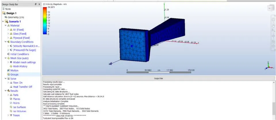
6. Steady Flow is assumed rather than transient as the time conditions are difficult to execute.

7. Also, the flow is assumed to Incompressible and turbulent, hence, turbulence models are employed.

i) Study A-Turbulence models and Material

Keeping the basis assumption in mind, the first study had the same model imported in Autodesk CFD,

Example of Result Valuation:

Velocity Plane:

but each time the turbulence specification used differed and the material used for components of Wind tunnel, differed too. The studies carried out for our analysis comprise of 4 turbulent models- K-epsilon, K-Omega, SST k-omega and LES Model on the preliminary base inspired design. The comparisons are then laid out with some proper inferences and conclusions.

Traces or Flow Visualization: Figure 38

With less coarse/seed of Trace: Figure 39

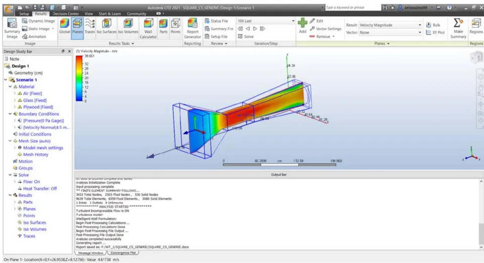
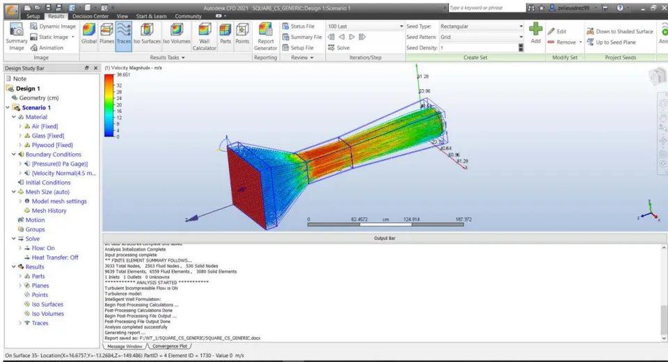
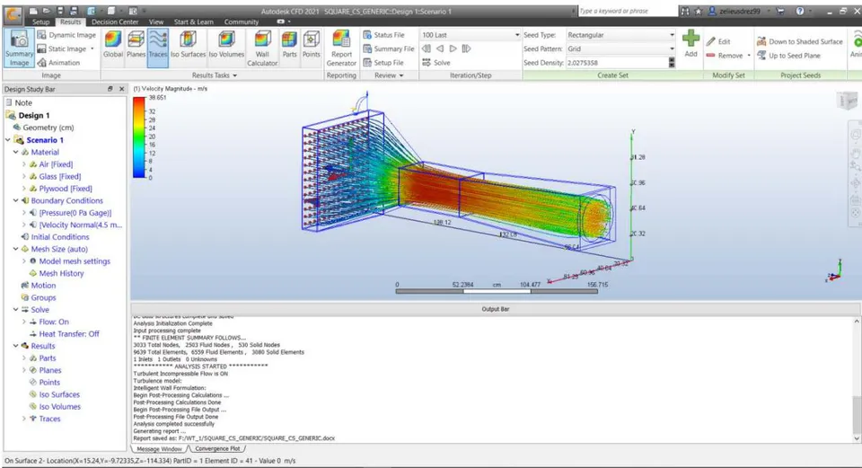
Tabular data with different turbulent models employed and material:

1. Plywood Contraction, diffuser and settling chamber with different test sections and Turbulence Models

Figure 40: Plywood Table with different turbulence models

MATERIAL USED		TURBULENCE MODELS -->		K-EPSILON	SST K-OMEGA	LES	LAMINAR
OTHER	TEST SECTION	PARAMETERS
PLYWOOD	GLASS	VELOCITY	X	754.536 cm/s	756.567 cm/s	750.624 cm/s	879.154 cm/s
			Y	753.112 cm/s	758.37 cm/s	746.656 cm/s	874.972 cm/s
			Z	620.577 cm/s	703.199 cm/s	818.29 cm/s	1948.63 cm/s
		T-D	MAX	150448000.0 cm^2/s^3	905059.0 cm^2/s^3	27.3952 cm^2/s^3	0
			MIN	27.3952 cm^2/s^3	1.52879 cm^2/s^3	1.0 cm^2/s^3
		T-K	MAX	330843.0 cm^2/s^2	653430.0 cm^2/s^2	253.125 cm^2/s^2
			MIN	1.817e-07 cm^2/s^2	0.0 cm^2/s^2	0.0001 cm^2/s^2
		PRESSURE	pressx	2644.3 dynes	16203.0 dynes	14472.0 dynes	-23984.0 dynes
			pressy	27319.0 dynes	15160.0 dynes	13243.0 dynes	-45657.0 dynes
			pressz	-40947000.0 dynes	-42514000.0 dynes	-44433000.0 dynes	-33559000.0 dynes
		SHEAR	shearx	88.773 dynes	-152.34 dynes	-3.9577 dynes	0.8264 dynes
			sheary	-7.0527 dynes	-26.774 dynes	-3.0545 dynes	-25.309 dynes
			shearz	-301670.0 dynes	-624360.0 dynes	-6706.1 dynes	-9575.5 dynes
	ACRYLIC	VELOCITY	X	754.626 cm/s	756.573 cm/s	750.622 cm/s	Laminar Flow is not considered as by reynolds's number, flow is turbulent, above shown laminar is only for comparison and should not be considered
			Y	753.236 cm/s	758.363 cm/s	746.655 cm/s
			Z	620.856 cm/s	703.228 cm/s	818.142 cm/s
		T-D	MAX	150454000.0 cm^2/s^3	905059.0 cm^2/s^3	27.3952 cm^2/s^3
			MIN	27.3952 cm^2/s^3	0.326481 cm^2/s^3	1.0 cm^2/s^3
		T-K	MAX	330784.0 cm^2/s^2	653437.0 cm^2/s^2	253.125 cm^2/s^2
			MIN	1.817e-07 cm^2/s^2	0.0 cm^2/s^2	0.0001 cm^2/s^2
		PRESSURE	pressx	4290.0 dynes	16159.0 dynes	14473.0 dynes
			pressy	26706.0 dynes	15189.0 dynes	13251.0 dynes
			pressz	-40942000.0 dynes	-42514000.0 dynes	-44433000.0 dynes
		SHEAR	shearx	90.554 dynes	-100.75 dynes	-3.9561 dynes
			sheary	-0.25071 dynes	-32.444 dynes	-3.0665 dynes
			shearz	-301610.0 dynes	-624300.0 dynes	-6706.1 dynes

2. Aluminium Contraction, diffuser and settling chamber with different test sections and Turbulence Models Figure 41: Aluminium Table with different turbulence models

MATERIAL USED		TURBULENCE MODELS -->		K-EPSILON	SST K-OMEGA	LES	LAMINAR
OTHER	TEST SECTION	PARAMETERS
ALUMINIUM	GLASS	VELOCITY	X	754.226 cm/s	756.628 cm/s	750.626 cm/s	879.158 cm/s
			Y	752.796 cm/s	758.425 cm/s	746.658 cm/s	874.982 cm/s
			Z	621.58 cm/s	703.216 cm/s	818.28 cm/s	1948.66 cm/s
		T-D	MAX	150461000.0 cm^2/s^3	905059.0 cm^2/s^3	27.3952 cm^2/s^3	0
			MIN	27.3952 cm^2/s^3	1.52902 cm^2/s^3	1.0 cm^2/s^3
		T-K	MAX	330903.0 cm^2/s^2	653417.0 cm^2/s^2	253.125 cm^2/s^2
			MIN	1.817e-07 cm^2/s^2	0.0 cm^2/s^2	0.0001 cm^2/s^2
		PRESSURE	pressx	5067.5 dynes	16193.0 dynes	14474.0 dynes	-23985.0 dynes
			pressy	26823.0 dynes	15208.0 dynes	13247.0 dynes	-45654.0 dynes
			pressz	-40931000.0 dynes	-42514000.0 dynes	-44433000.0 dynes	-33559000.0 dynes
		SHEAR	shearx	88.634 dynes	-139.04 dynes	-3.9577 dynes	0.82472 dynes
			sheary	-0.0089166 dynes	-16.825 dynes	-3.0609 dynes	-25.285 dynes
			shearz	-301560.0 dynes	-624360.0 dynes	-6706.0 dynes	-9575.1 dynes
	ACRYLIC	VELOCITY	X	754.564 cm/s	756.563 cm/s	750.623 cm/s	Laminar Flow is not considered as by reynolds's number, flow is turbulent, above shown laminar is only for comparison and should not be considered
			Y	753.167 cm/s	758.376 cm/s	746.656 cm/s
			Z	622.894 cm/s	703.196 cm/s	818.253 cm/s
		T-D	MAX	150465000.0 cm^2/s^3	905059.0 cm^2/s^3	27.3952 cm^2/s^3
			MIN	27.3952 cm^2/s^3	1.48268 cm^2/s^3	1.0 cm^2/s^3
		T-K	MAX	330789.0 cm^2/s^2	653436.0 cm^2/s^2	253.125 cm^2/s^2
			MIN	1.817e-07 cm^2/s^2	0.0 cm^2/s^2	0.0001 cm^2/s^2
		PRESSURE	pressx	4883.5 dynes	16219.0 dynes	14475.0 dynes
			pressy	26235.0 dynes	15240.0 dynes	13250.0 dynes
			pressz	-40943000.0 dynes	-42514000.0 dynes	-44433000.0 dynes
		SHEAR	shearx	88.823 dynes	-118.73 dynes	-3.9588 dynes
			sheary	-0.048968 dynes	-22.677 dynes	-3.0655 dynes
			shearz	-301600.0 dynes	-624270.0 dynes	-6706.0 dynes

3. Legend or Index for Navigation

Figure 42: Legend for data

LEGEND
Acronym	Full Text	Depiction
K-E	K-Epsilon Model	TURBULENCE MODELS
SST K OMEGA	Shear Stress Transport K-turbulence model
LES	Large Eddy Simulation or Eddy Viscosity Model
LAMINAR	Laminar Flow	NON TURBULENT
T-D	Turbulence Density	RESULT PARAMETER
T-K	Turbulence Kinetic Energy

INFERENCE TABLE:

Figure 43: Table of Inferences for Study A

INFERENCES FROM MATERIAL
1. Although laminar is seen in the above table, flow is turbulent and should be ignored.	VELOCITY
2. Velocity in X direction does not vary by a vast amount when test material is switched from glas to acrylic, and by a negligible amount when switch from
3. Velocity in Y direction gives the same results
4. Velocity in Z direction is same for most of the models and materials, but is the highest for LES Model
5. Turbulence Density (T-d) is same for all materials, highest turbulence is found in K-Epsilon Model while LES gives the least turbulence, which makes LES a	T-D
6. Turbukence Kinetic Energy (T-k) gives similar results to T-d, thus the scale again, tips towards LES	T-K
7. For all turbulence models, Pressure in X direction increases when acrylic is used except for Aluminium	PRESSURE
8. Pressure in Y direction also increases when acrylic is used except for K-E Model
9. Pressure in Z is almost equal regardless of model and material, but negative
10. Shear in X direction is negative for SST K Omega and LES	SHEAR
11. Shear in Y and Z direction is negative for all turbulence models
12. Shear in X and Y direction reduces when Aluminium is used
13. Shear in Z direction remains same for material

Conclusions of Study-A

1. Velocities, T-D and T-K are almost similar for most of the models used.

2. LES (Large Eddy Simulation or Viscosity) is the model with least turbulence and will be selected as primary basis for comparison in geometry part of the study.

3. Although the pressure/Shear reduces by a very small amount, glass or acrylic both give same result.

4. Aluminium does give a very slight increase in velocity, but trading for cost value, given that for same cross section, Plywood is Rs. 950 while Aluminium is Rs.1650, plywood is favoured and recommended as it provides equivalent results.

Contraction Cone with $3^{rd}$ degree polynomial

LES Models are sufficient with lesser turbulence and plywood is an affordable, effective material for wind tunnel along with Glass as the test section. LES model is thus, the preferred choice of computing flow and Plywood with glass test-section, the go-to materials.

j) Study B-Geometry

Using the same materials, as stated above, plywood contraction, diffuser and settling chamber but with glass test section, as well as the same set of basic assumptions and constant boundary conditions, we carry out studies implementing different scenarios. The scenarios are Geometry change-Circular diffuser, Octagonal Contraction, Contraction with different wall shape-polynomial.

As component

Assembly with Square diffuser

Model with material in Autodesk CFD Figure 47

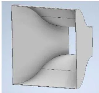
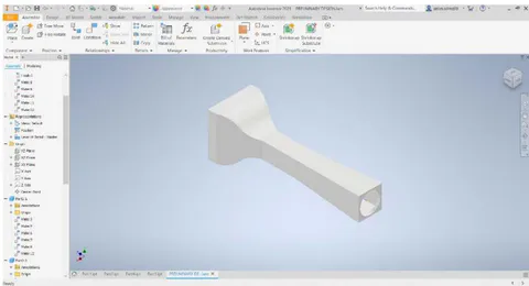
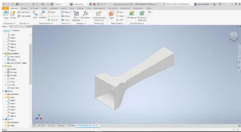
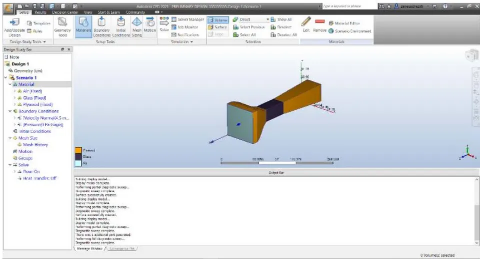
Velocity profile and Flow field around model

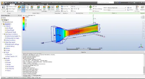
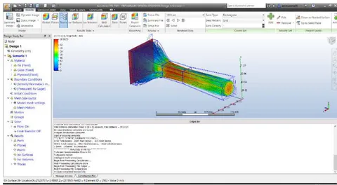
Contraction curve with $3^{\text{rd}}$ degree of curve of wall Similar to $3^{\text{rd}}$ degree contraction curve results and analysis are developed for $5^{\text{th}}$ degree curve. As component

As assembly with material, and square diffuser

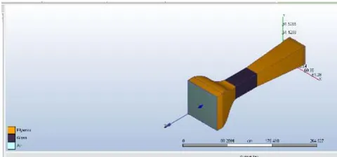
Octagonal Contraction cone with square diffusers and test section Assembly with material

Figure 52 Velocity Profile

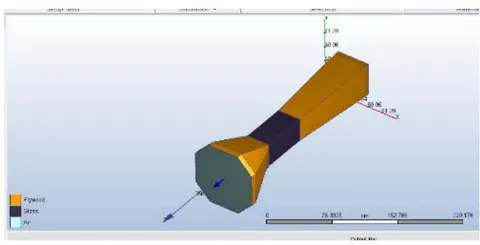
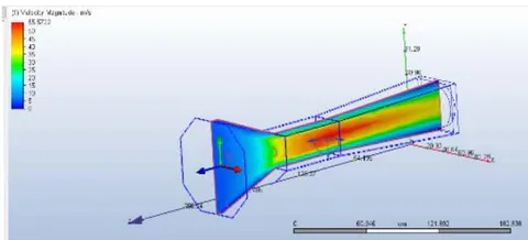
Circular diffusers with a. Square Cross section Contraction chamber

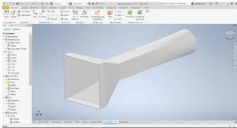
b. Square cross section with $3^{rd}$ degree and $5^{th}$ degree wall curves

Figure 58 Important Note One must avoid leakage errors as shown below in the figure. The CFD would never process under such conditions

The $5^{\text{th}}$ and $3^{\text{rd}}$ Degree polynomial curves are different in a very small aspect:- The steepness of curve, figure below shows the plot of the same. Blue is the cubic polynomial. Tabular Data of collected conditions of geometry

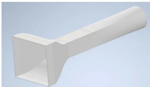
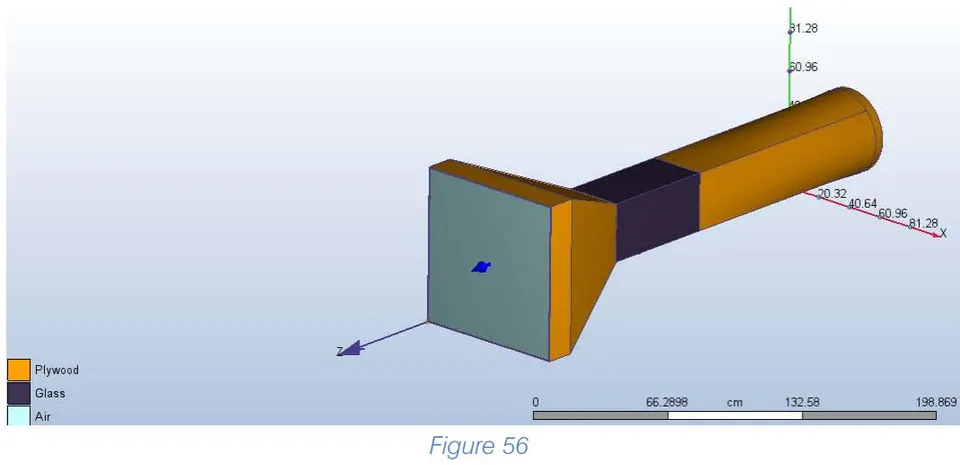
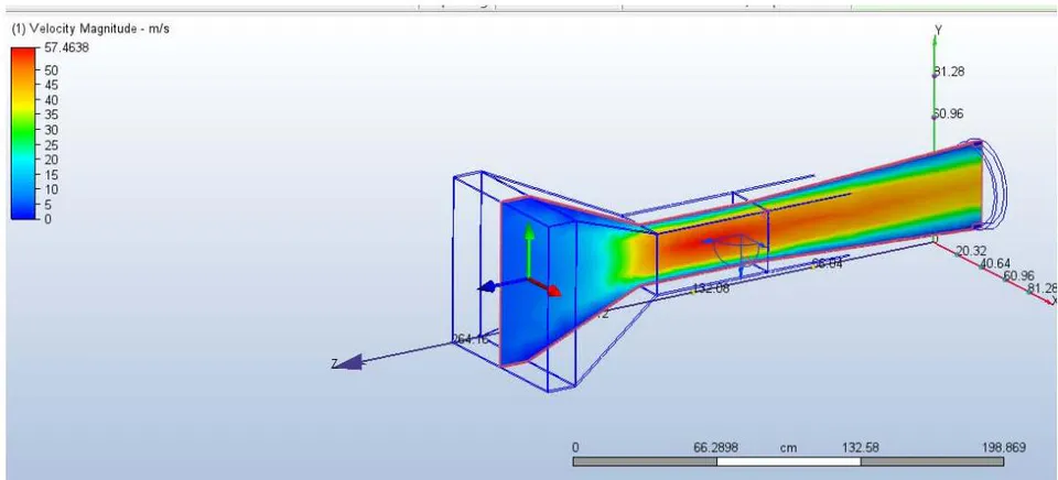
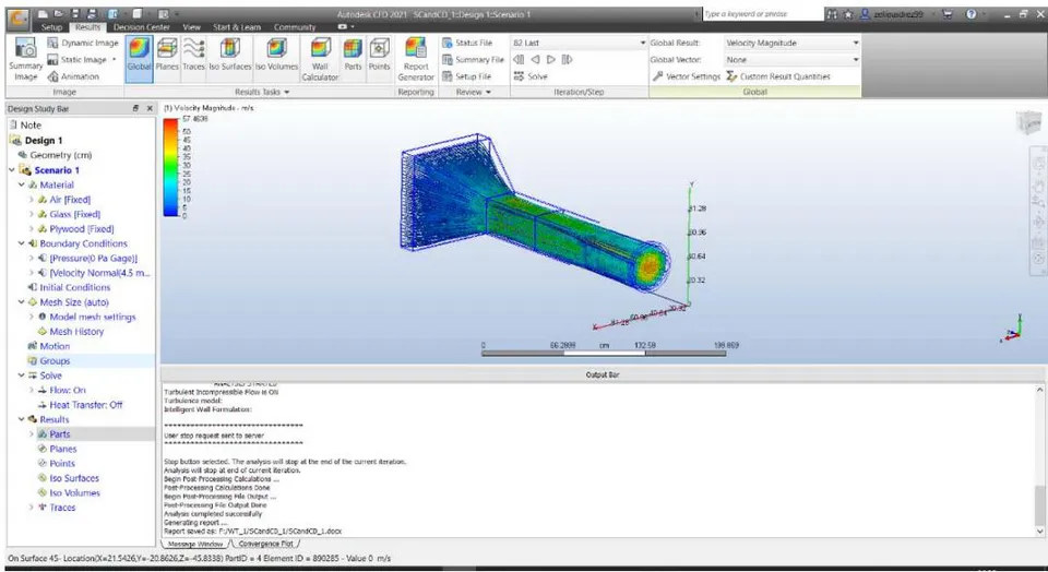
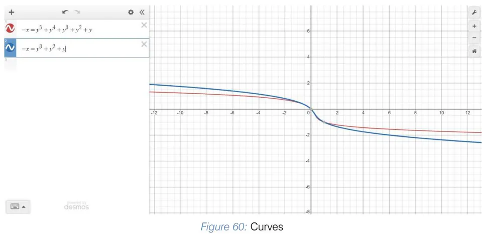
Square Contraction with 3rd degree wall curve polynomial

GEOMETRY - STUDY B

GEOMETRY

PARAMETERS -->

VELOCITY

T-D

T-K

PRESSURE

SHEAR

CONDITIONS

X

Y

Z

MAX

MIN

MAX

MIN

pressx

pressy

pressz

shearx

sheary

shearz

CONTRACTION CHAMBER

Square contraction chamber

Square test section, settling chamber, and generic diffuser.

750.625 cm/s

746.648 cm/s

818.217 cm/s

27.3942 cm^2/s^3

1.0 cm^2/s^3

253.125 cm^2/s^2

0.0001 cm^2/s^2

14421.0 dynes

13212.0 dynes

-44433000.0 dynes

-3.8814 dynes

-3.0763 dynes

-6706.1 dynes

Square Contraction with 3rd degree wall curve polynomial

930.12 cm/s

784.446 cm/s

823.952 cm/s

27.4036 cm^2/s^3

1.0 cm^2/s^3

253.125 cm^2/s^2

0.0001 cm^2/s^2

1279.2 dynes

18962.0 dynes

-46825000.0 dynes

-5.4671 dynes

-21.526 dynes

-6617.1 dynes

Square Contraction with 5th degree wall curve polynomial

920.204 cm/s

692.823 cm/s

847.677 cm/s

27.3956 cm^2/s^3

1.0 cm^2/s^3

253.125 cm^2/s^2

0.0001 cm^2/s^2

10055.0 dynes

9323.0 dynes

-44021000.0 dynes

-6.6323 dynes

-5.9466 dynes

-6584.8 dynes

Octagonal Contraction chamber, thickness of octagonal start is 3 inch.

Square Test section and generic diffuser, but no settling chamber

734.611 cm/s

782.598 cm/s

823.574 cm/s

9.44916 cm^2/s^3

1.0 cm^2/s^3

253.125 cm^2/s^2

0.0001 cm^2/s^2

667.36 dynes

15876.0 dynes

-63782000.0 dynes

21.73 dynes

-43.307 dynes

-82265.0 dynes

DIFFUSER

Generic Diffuser, Square cross section

Square test section, settling chamber, and Straight Square contraction Cone

750.625 cm/s

746.648 cm/s

818.217 cm/s

27.3942 cm^2/s^3

1.0 cm^2/s^3

253.125 cm^2/s^2

0.0001 cm^2/s^2

14421.0 dynes

13212.0 dynes

-44433000.0 dynes

-3.8814 dynes

-3.0763 dynes

-6706.1 dynes

Circular diffuser

Square test section, settling chamber, and 3rd degree polynomial curve of walls of Square contraction Cone

675.358 cm/s

677.719 cm/s

863.25 cm/s

32.5923 cm^2/s^3

1.0 cm^2/s^3

253.125 cm^2/s^2

0.0001 cm^2/s^2

16204.0 dynes

6728.4 dynes

-103220000.0 dynes

51.077 dynes

68.879 dynes

-177060.0 dynes

Square test section, settling chamber, and 5th degree polynomial curve of walls of Square contraction Cone

743.177 cm/s

681.398 cm/s

872.69 cm/s

32.5923 cm^2/s^4

1.0 cm^2/s^4

253.125 cm^2/s^3

0.0001 cm^2/s^3

-39929.0 dynes

3790.1 dynes

-105820000.0 dynes

115.51 dynes

-205.29 dynes

-184590.0 dynes

NOTE:

Assumed thickness=0.25inch, Incompressible flow, LES Turbulence Model, Automatic Mesh, Plywood Other components, and glass test section. Test Section is same throughout all models.

Conclusions and Inferences

1. When the contraction degree of wall curve is increase the cross flow due to velocity in X direction does increase by a small amount.

2. The turbulence energy dissipation and Kinetic energy of turbulence remains same.

3. Pressure along Y direction decreases as the wall curve degree increases.

4. Shear is in negative and is neglected.

5. The octagonal contraction chamber surges the velocity in Z direction with a focused flow by curtailing velocity in X and Y directions.

6. The pressure on the wall (Y-direction) escalates by a small amount when Octagonal test section is used rather than square peculiarly the one with 5th degree curve.

7. In case of diffusers, velocity fluctuations are reduced when circular cross section ones are implemented rather than the square ones.

8. Moreover, when circular cross sections are used, velocity in Z-direction also soars, with better velocity profiles.

9. Pressure reduces on the walls (Y direction) when square cross section with 5th degree curves are utilized with circular diffusers but on the cost of shear.

10. Thus, a good tip in the balance would be towards a square contraction cone with 5th degree curve and a circular cross-section.

k) Study C- Other Scenarios

Include, increasing length of settling chamber, changing thickness of plywood and reducing length of test section.

Tabular data of variations Figure 62: Tabular data of Study C

SCENARIO-STUDY C

SCENARIOS

PARAMETERS ->

VELOCITY

T-D

T-K

PRESSURE

SHEAR

X

Y

Z

MAX

MIN

MAX

MIN

pressx

pressy

pressz

shearx

sheary

shearz

DIFFERENT THICKNESS OF PLYWOODS (IN INCHES)

Varying Thickness of Plywood

0.25

750.625 cm/s

746.648 cm/s

818.217 cm/s

27.3942 cm^2/s^3

1.0 cm^2/s^3

253.125 cm^2/s^2

0.0001 cm^2/s^2

14421.0 dynes

13212.0 dynes

-44433000.0 dynes

-3.8814 dynes

-3.0763 dynes

-6706.1 dynes

0.5

744.415 cm/s

748.805 cm/s

814.825 cm/s

28.0373 cm^2/s^3

1.0 cm^2/s^3

253.125 cm^2/s^2

0.0001 cm^2/s^2

-29619.0 dynes

4595.3 dynes

-45150000.0 dynes

4.8144 dynes

-5.9991 dynes

-6474.7 dynes

0.75

802.979 cm/s

805.256 cm/s

720.951 cm/s

28.0373 cm^2/s^4

1.0 cm^2/s^4

253.125 cm^2/s^2

0.0001 cm^2/s^2

-39130.0 dynes

13238.0 dynes

-46563000.0 dynes

13.287 dynes

-8.3238 dynes

-6054.8 dynes

TEST SECTION LENGTH VARIED (in Feet)

REDUCED TEST SECTION LENGTH

2FT

750.625 cm/s

746.648 cm/s

818.217 cm/s

27.3942 cm^2/s^3

1.0 cm^2/s^3

253.125 cm^2/s^2

0.0001 cm^2/s^2

14421.0 dynes

13212.0 dynes

-44433000.0 dynes

-3.8814 dynes

-3.0763 dynes

-6706.1 dynes

1FT

741.449 cm/s

731.889 cm/s

839.382 cm/s

27.3906 cm^2/s^3

1.0 cm^2/s^3

253.125 cm^2/s^2

0.0001 cm^2/s^2

18672.0 dynes

15429.0 dynes

-43079000.0 dynes

-5.6367 dynes

-5.4169 dynes

-5423.0 dynes

LENGTH OF SETTLING CHAMBER VARIED (IN INCHES)

INCREASED LENGTH OF SETTLING CHAMBER

6IN

750.625 cm/s

746.648 cm/s

818.217 cm/s

27.3942 cm^2/s^3

1.0 cm^2/s^3

253.125 cm^2/s^2

0.0001 cm^2/s^2

14421.0 dynes

13212.0 dynes

-44433000.0 dynes

-3.8814 dynes

-3.0763 dynes

-6706.1 dynes

12IN

737.505 cm/s

748.881 cm/s

900.96 cm/s

27.4057 cm^2/s^3

1.0 cm^2/s^3

253.125 cm^2/s^2

0.0001 cm^2/s^2

2124.7 dynes

-11972.0 dynes

-44876000.0 dynes

0.24949 dynes

1.2893 dynes

-6914.9 dynes

NOTE:

Assumed Incompressible flow, LES Turbulence Model, Automatic Mesh, Plywood for other components, and glass test section. Square contraction chamber, settling chamber, test section and diffusers used.

Conclusions and Inferences

1. Using lesser thickness of Plywood increases velocity in test section as seen from $V_z$.

2. In other words, the larger thicknesses of plywood, increase the resistance to flow of Wind.

3. The distribution towards X, Y directions of velocity increases as thickness of plywood increases.

4. The value of T-K and T-E remain more or less the same, irrespective of thickness.

5. The reduction of test section, increases velocity by a slight amount but on the expense of higher pressure and reduced test section area to place model.

6. The increase in the length of settling chamber does help reduce pressures inside tunnel, with higher uniformity, but the shear forces rise. The velocity achieved in the test-section, too, increases.

7. Thus, the optimal thickness would be that of 0.25 inch of plywood, proper length of test section would be 2ft, meanwhile a compromise for settling chamber would be 7 inches.

IX. FINAL DESIGN AND SPECIFICATIONS

As mentioned, material chosen was glass for the test section, plywood for the components of wind tunnel. The contraction cone is square but with a $5^{th}$ degree polynomial curve for the walls. The test section is square. The diffuser is circular. Settling chamber is employed at the start with Honeycomb mesh and screen to reduce the turbulence. Thus, these components are shown below and modelled in Inventor.

a) Components

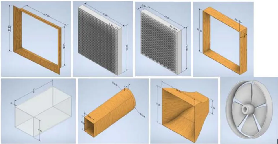
c) Overview

b) Exploded view

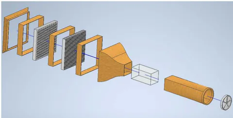
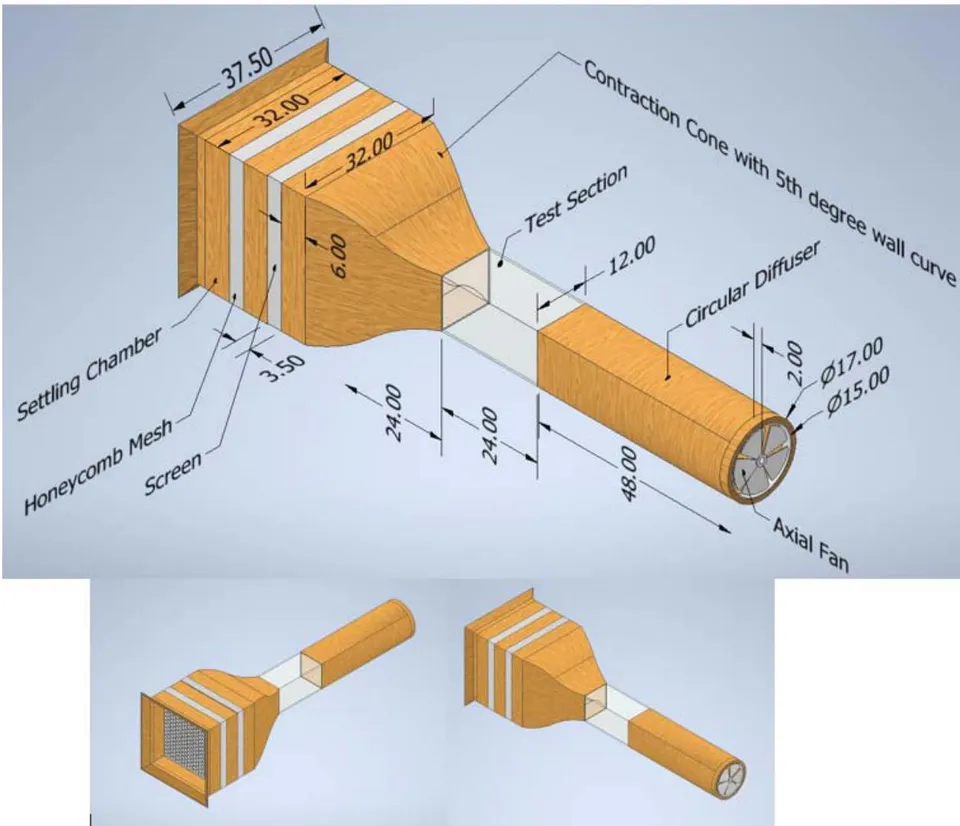
X. THE NEXT STEPS

The consequent step after the design would be the manufacturing of the tunnel for college and research purposes.

A structure can be adopted to keep the wind tunnel mounted. Aluminium pipes could be adopted for honeycomb mesh due to its low weight, and considerable strength. Nails and bonds with adhesive glue seems considerable enough as well. For the plywood constructed diffusers, along with holding structures, dampers could be used to absorb the vibrations. It is important to check for leakages of air as well. [9, 10]

Piano hinges could be used open and close test section windows made from plexi glass. Digital scales over mechanical being superior could be employed if the budget is suitable

There is a formidable amount of effort required for the selection of fan, especially the variable frequency part, seems a little onerous, but provides very good ranges and test velocities. The motor could be mounted in special hub casing with blades from aluminium if needed, to reduce the weight of tunnel. Controllers are implemented to operate the fan properly. Entire structures and wind tunnel mountings could be even placed on tables for feasibility if need be.

Based on "Memento des pertes de charge: Coefficients de pertes de charge singulièreset de pertes de charge par frottement", by I.E. Idel'cik [Eyrolles, 1986], authors of [18] have presented an aided spreadsheet as well, for helping with the design of closed wind tunnels. Dimensioning schemes are present on excel spreadsheet on "http://www.aero.upm.es/LSLCWT"

Thus with these beneficial and profound aspects, the designed model could lead to the effective learning and practical applications of the concepts mentioned.

One can additionally, investigate pressure distribution for drag reduction or enhancement of life. There is also, mention for self-correcting wind tunnels in transonic zone, where the blockage could be alleviated by ventilating wind tunnel walls $[25,18,8]$.

Some papers like $[46]$ mentioned studying ice accumulation on airplane wings, which could be studied for e.g. NASA Glenn Wind tunnel. Possibly an area of future research could be "Plasma actuation", a technique of actively controlling airflow. $[48]$

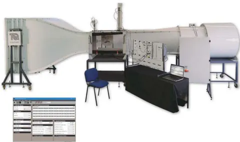
XI. CONCLUSIONS

Although a condition such as the end of diffuser being square but with circular fan poses a disturbance of airflow, this effect is negated with axial fan.

Thus, this paper tries to provide the right guidelines one could utilize for design of an Open circuit Wind tunnel. The right material and geometry with discussions using Autodesk Inventor and Autodesk CFD have been presented.

The Study A using different turbulent models helps give a picture about pattern of fluif flow distribution in test chamber with superiority of each model complementing each other.

Moreover, the confabulated Wind tunnel foreshadows so many research principles and R.D Mehta notes, hence, this design would suffice as a research tool in field of fluid mechanics and is not limited to just that.

ACKNOWLEDGMENT

The authors acknowledge and express their gratitude towards the various research scholars for their foundational work and contribution to such an enormous field. The authors also, are grateful towards peers and our project mentors.

2. Internal aerodynamics corresponding to flow movement inside the body, such as through ducts, turbines and piping.