I. INTRODUCTION
Earthquake focus location procedures and its applications had appeared long before the XIX century. Automated procedures and wide-scale use of it were appearing in the middle of the XX century. So it may seem that we should know all about location procedures itself and Earth interior, nothing new can be found in this way.
Nevertheless, it turned out - something new may be found at hand. Detailed analysis showed that new is hidden in the velocity structure of the crust and upper mantle. It comes from here into generalized seismic travel tables fluently.
To be honest, this requires time, power computers, digital seismic records and time synchronization of seismic recorders.
The work is based on data processing of seismic records obtained from different agencies. Most seismological investigations deal with particular seismic events. In our case we have analyzed the process of location itself, and try to generalize the results to have as comprehensive as possible valuable algorithms.
We had been searching common intermediate appearances of some dependencies of the time delaying from depths when such dependencies were found. The object of investigation was changed at that moment: instead of location procedures the model of crust seismic events became the object of investigation.
At the same time, we meet with disagreement: the result of seismic event location is a point. For the earthquake appearance it is required that in its sources were presented the movements of a big mass of material with varying acceleration. That generates enough kinetic energy to produce an observed action as an earthquake. This point gives a start to changing the direction of the investigation. We began searching for a way to describe the focal zone model in terms of energy.
Now, we can talk about the tools we used in this investigation. At first, we were using a standard location algorithm. This work uses a modified Geiger algorithm of location ([Geiger, L., 1912]), supplemented with the simplex method ([Ge, M., 1995]; [Prugger, A., et al., 1989]).
Work carried out in a frame of investigation of the ability to elaborate automated determination of the core events depth. Nevertheless, we were trying to find the ability to work terms energy .
II. RUPTURE LINE
Geiger method permits finding the location of most seismic events if they have enough arrivals starting from an arbitrary hypocentre approach. But almost near the final point of the solution the convergence began to decrease. To understand the reason that led to such behavior, the location algorithm was changed on the final steps. The Geiger method was changed by the simplex method which was combined with a fixed depth calculation procedure. This procedure consequently changes depth with fixed steps for each new hypocentre location.
The result showed that hypocentres were lining up to the chain. Analysis indicated that chan's links form a smooth line. This effect was observed for all processed events. This line is located in 4D space: three 3D space coordinates and time. But only two of four coordinates have significant meaning – depth and time. This is a common property for any set of first arrivals of the same seismic event. We named this effect "rupture line". It is not a line of rupture in reality. This line is the locus of hypocentres obtained by the location procedure.
Strictly speaking, a rupture line is a structure or object (from algorithmic points of view). An element of this structure involves several parameters. Each element corresponds to hypocentre location. Mathematically, it may be written as:
where a function that determines parameters of the structure elements. First forth parameters determined hypocentre location. Fifth parameter is a mean square root residual (RMS). This parameter defines the quality of the location solution. We can write expressions for RMS as:
where - epicentre parameters, - a trail depth, - phase residual, - index of seismic phase, - total phase number, - number of independently defined parameters. Phase residual is:
where - phase residual dependent of epicentral distance and trail depth; -observed time arrival of phase , -calculated time arrival for phase which is dependent from epicentral distance and depth and may be obtained from travel time tables. The last summand - presents uncertainty of measurement of 's time arrival. Uncertainty of the measurement should be present in expression of a phase residual, but it may be put to zero without loss of generality during formal expressions manipulations.
The calculated time arrival may written as , where - origin time, -a function to calculate time delaying by travel time tables. Now we can write an expression for the first argument in (1):
where argument in last term -is a phase origin time, the angle brackets means the operator taking the average of the argument. As usual, algorithms that use the Geiger method or simplex technique are fined a value of the origin time by averaging the middle term of expression (4). Expression (4) indicates dependencies between parameters from structures of different types – the first structure is a rupture line; next is discussed in the next section.
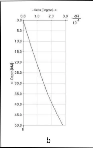
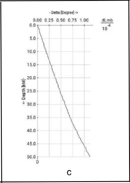
Fig. 1 presents the graphs of three coordinates of the rupture line - origin time (a), latitude (b) and longitude (c). Fourth coordinate - depth is a parameter (vertical axis). Two coordinates are parameters of the structure - origin time and depth. It means that any one of these parameters define location along this structure. The last indicates strong dependencies of these two parameters. That is vital for our further considerations. The presented result was obtained from the data processing of the event 2022.01.7 17:40:34 in China. It is essential that dependencies for space coordinates from depth are weak. This deviations from a straight vertical line originated by in homogeneity of media of propagation seismic waves and due to discrepancy Globe with ideal sphere form - deviation value in (arc degree) corresponds to .
III. CHARACTERISTICS
The last term in expression (4) does not contain parameters of a rupture line. At the same time, the first term is rupture line parameters only.
This leads us to mind: maybe we have another linear structure similar but differs from the rupture line?
If in expression (4) we have structure in the left side and averaging operator of set of structure parameters in right, it quickly suggests that structures in argument in the right side have the similar behaviour to the structure in the left of (4).
For time arrivals can be written following expression:
In the previous investigation was found: if than for any .
This assertion should be proven. But travel time tables obtained experimentally. So proving shall be based on comparing the results of data processing.
Let us write the expression:
where is the number of the seismic records, - is a thickness of crust and upper mantle;
The expression (6) defines a mathematical set; let's call it a phase characteristic. Term phase means that we have such a set of for each of the phases we are mentioned in the article. The set is similar to rupture line structure. The difference is that contains information from all arrival of the event, when each characteristic is connected only with one arrival.
Another similarity is that a characteristic element consists not only of parameter , but of the following parameters , where - a phase origin time, - the depth along the characteristic, - is arrival time, - arrivals amplitude. The parameter defines uniquely due to it being constant within characteristic. The params and define location along characteristic.
From (5), we can write
This expression consists of absolute time in terms of and . To simplify comparing, we subtract from both these terms (or from the left and right side of the expression (7)). Such a way, we got relative time expressions. It will be used later.
Now, we can compare the relative phase origin time values with the relative origin time values along the rupture line. We will be presented on a graph below the relative values of parameters only. We will be implied as a subtrahend parameter value on zero depth, if the opposite does not indicate.
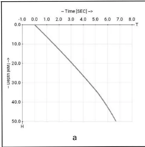
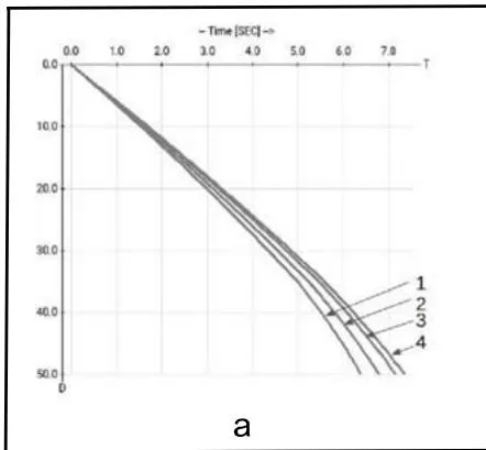
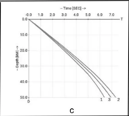
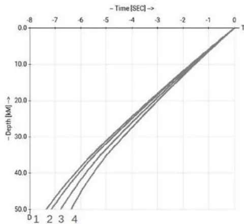
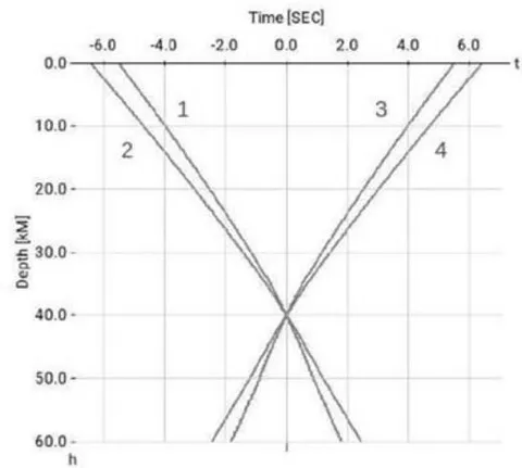
Fig. 2 present the dependence from depth of the origin time on a characteristic . Fig. 2.a are presented graphs for four epicentral distances. The epicentral distances are: line , line , line , line .
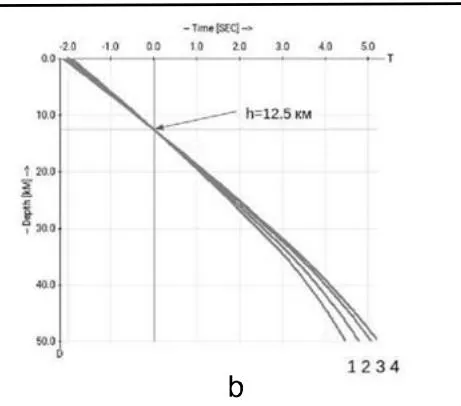
Fig. 2.b are presented graphs for the same epicentral distances, but as a subrahend was taken the origin time at depth . It is demonstrated that characteristics cross in one point corresponds to the focus depth. Fig. 2.c. presented comparing the dependence of a depth of the origin time on the characteristics and the origin time on the rupture time. Line 1 is the characteristic origin time with , line 2 is the characteristic origin time with ; line 3 is the rupture line origin time. The results obtained for the event 2022-01-07 17:45:34 in China.
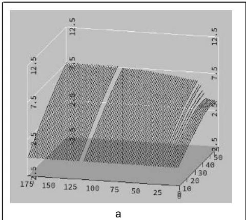
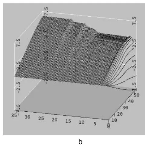
We can see on Fig. 2 that slope of a characteristic is changing with a changing of epicentral distance. Fig. 3 demonstrates in 3D projection two arguments function which are obtained from (7) by eliminating absolute time.
We can see that the region of available epicentral distances splits into some zones. Two of them have smooth dependence on epicentral distances. This requires certain restrictions during the picking up of the seismic stations for data processing.
IV. LOCAL UNIT FOR MEASUREMENT OF ENERGY SIMILAR VALUES
The value of calculated along the rupture line might have not a minimum for some events in a reasonable interval of the depth. This does not mean that (2) is not working. It means that uncertainty of residuals in (3) in dependencies of the depth is large. Another reason may be unsuccessful selection of seismic stations. We will discuss this later. In this work we are very wide using this criteria for location procedure with fixed depth values. Coordinate location procedure finds out the minimum of value of always.
In this work, we will not concentrate on the problem of why the above might happen (see also [Dmitry Storchak, 2011] and [Engdahl, E.R., et al., 1998]). This is a well-known fact. This work suggests different criteria for the final solution. The suggestion is based on using a physical indicator. Such an indicator may be seismic energy (or value with similar properties) emission from the focal zone.
The final hypocentre is located on the rupture line in the point where seismic energy reaches maximal value. Actually, the rupture line is a locus of points of minimum expression (2) with fixed depth. This is coincidental with traditional location procedures. We are refusing to search the minimum of (2) by the depth and suggested searching the maximum of the energy radiations along the rupture line.
As an energy similar object, we are choosing the "amplitude parameter" or for short . Its expression is
where - spectral amplitude, - spectral frequency, sampling interval, frequency index, - one side frequencies number of Fourier transforming (for positive and negative frequencies, it has the same value (see Appendix A)); - phase index and - number of seismic records. is calculated separately for each phase.
has physical dimension . If value multiply to granite density on the Earth's surface, we will get dimension . So, the seismic radiation energy in Jouilies may be obtained by integration over the volume of the focus zone (this requires knowing how the energy radiation is distributed over the focal zone) and over the time of focus zone activity.
Desired algorithm was created. The algorithm is included another algorithm to calculate coherence in every point of the focus zone1. The last algorithm is a central part of described development. The vital ability of that algorithm is that it permits defining the main part of the spectral window. The main part is defined by the maximum coherence value. Appendix A describes it.
The physical dimension is . It is not an energy yet, but relations of two such values give us the same result as a relation of energy values. may be used for comparing relation values instead of energy in the frame of one event.
The first problem formulated in the frame of this work is a determination of the depth of crust events. The depth of the event may be determined by searching the maximum of seismic radiation along the rupture line. Unfortunately, we have an impenetrable obstacle – amplitude along characteristic is constant.
V. DEPTH PHASE PP
The determination of the event depth depends on the answer to the question: what is the depth of the seismic event? Traditionally, this parameter was taken from the mathematical solution of a location task. Unfortunately, this determination of term depth ignores physical aspects of earthquake phenomena.
This work suggested using depth value which corresponds to maximal radiation of seismic energy along rupture line. Considering, that amplitude along characteristics are a constant it is possible to use another phase. The depth phase may be used instead of the phase. phase has the same focus impulse as a phase .
Fig. 4 shows the graphs of characteristics phase origin time in dependency of depth - continues lines and from epicentral distances - separated lines. The essential property of characteristics is that its derivative of phase origin time by depth is negative while phase origin time derivative is positive. These two types of characteristics are crossing in a compact area of 4D space. Later, we will examine this phenomenon in detail.
Before the next step, we rewrite expression (7) to make it clearer to which phase we mean
where is the seismic phase name: or .
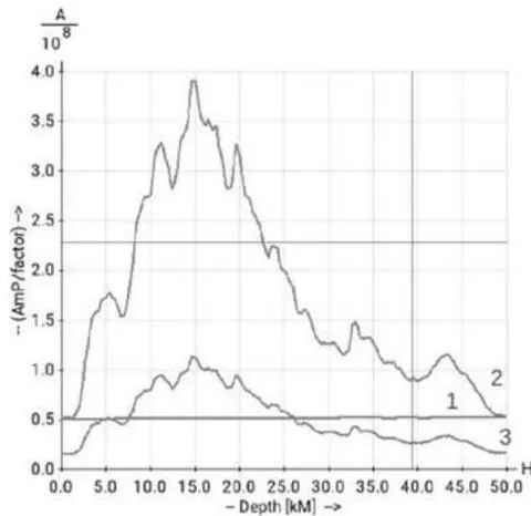
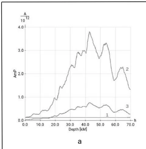
The result of the location procedure is presented in Fig. 5. This result was obtained from processing of the data of the event 2022-01-07 17:45:34 in China. That is an example of using both seismic phases and . Fig. 5 presents three graphs of : curve 1 - graph of , curve 2 - graph of , curve 3 - graph of expression.
where - index along rupture line and - number of points where was calculated; the value is the reproduction of the values of by scaling . Thus, we are taking into account the difference in amplitude of vertical components of a direct wave ( phase) and a reflected wave ( phase). Thus, we are bypass restrictions connected with the property of the characteristics. Expression (9) presents the algorithm of amplitude coordinations.
The maximum on the curves 1 and 3 define depth value , while USGS defined depth for this event as .
So, we see that developed algorithms are working. Let us now clarify how it works.
VI. THE SOLUTION SPACE AND FRAME REFERENCE
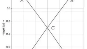
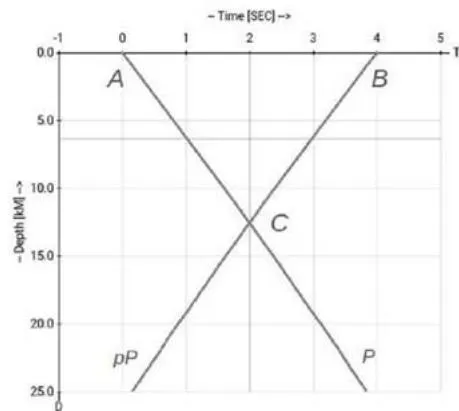
The schematic chart in Fig. 6 shows the collaboration of two dedicated seismic phases. First, we consider the frame reference of our solution. It is not a pure physical frame reference. 3D physical space will stay without changes. The fourth axis is a time. Chart in Fig. 6 is a slice of 4D space by a time-depth plane7. Line and its continuation is the time axis. The line and its continuation is characteristic; the line and its continuation is characteristic. It is drawn only one pair of characteristics belonging to the same record: we suggest that each recorder registered a pair of arrivals which can be detected as phases and . We are assuming that two seismic phases always exist and therefore two characteristics exist too. The point is a place where these two characteristics are crossing. According to the property of characteristics, the AmP along each of them are constant. What is the AmP value in point ? It looks like we have a contradiction.
In reality, The source is located at the point . The seismic radiation reaches the recorders with different amplitudes due to differences of the travel ways including radiation pattern. Hence, does not equal to .
There are two solutions to the mentioned problem that are presented in this work. One was demonstrated in connection with location procedure. Second will be considered later.
Each element of characteristics contains both parameters: and . First is the parameter which defines location along characteristic, second is a constant along characteristic. Value of event origin time is the averaging value of all characteristic parameters .
Let us segment or are the generalized characteristics: point will be an origin time of phase ; point will be an origin time of phase . Point is a place of crossing of both characteristics.
Let us introduce the value as a fixed value of the focus depth. Another meaning of the parameter is a focus depth. This segment may be a characteristic of phase or a rupture line.
In this case, It means all characteristics and the rupture line are crossing at the point in 4D space.
Let us named of abscissa axis (time axis) as . In this case, we can write for point expression . The same expression we can write for point . According to (7) and to the fact that we have If then . With depth increase the point will be moved from point to the right.
We can write for next:
and It easy to see that the distance of time between values and for depth is
The expression (10) is essential for our following consideration. We can formally use (10) to define the depth at the point by the difference between the time and
The solution frame reference consists of the 3D physical space and relative time.
VII. APPLYING DERIVED MATHEMATICAL INSTRUMENT FOR INVESTIGATION OF THE SEISMIC EVENTS FOCAL ZONE
This work was intended to improve depth location only. Eventually, we understood that our focus model should be improved too. Above, we described the procedure of determining events depth by applying amplitude parameters. The expression (9) converts the value of the into a . The last corresponds to the intensity of phase. Thus, the new location algorithm was preserved to be close to the traditional one. Graphs on Fig. 5 show the level of seismic radiations along the rupture line. The last was obtained by data processing of an event's records.
The next step was an attempt to apply an amplitude parameter for generalizing the station's seismic records. It shows the relative radiation intensity for active (coseismic) time period. It shows that the curve of the seismic activity has one maximum impulse and several impulses of less intensity. The less intensity impulses are the appearance of an internal sub-focus. The last achievement is ability to plot distribution of the intensity of inner sub-focuses. All this expansion was derived on the basis of mathematics described above.
The basis of algorithms is described above triangle (Fig. 6). The line is a part of the rupture line. Rupture line depends on the event's origin time, which depends on arrival times. If we forget about arrival times and will be changing origin time our geometrical construction that involves triangles will be moving along a time axis as a single object ( is a number of recorders). In this case, inverse rec calculations of new arrival times give the ability to take the amplitude parameters for new origin time. Thus, we can move along the time axis. The 3D space movement may be done by similar procedure.
It is possible to use all properties of the rupture line and all characteristics in the new time and space position. We can do it due to the fact that the parameters of our geometrical construction depend on the permanent data only.
Let us repeat the vital property: the value of parameters of the characteristic element are constant. According to this, the value of the parameter on characteristic for depth zero will be translated to point . We considered it early.
At the point we have two values. The problem is: how is it possible to agree on these two values? We used the following expression:
where -resulting amplitude parameter value for each point on choosing subspace, -index of the seismic records, -number of records. That is another variant of the algorithm of amplitude coordinations. First was presented as expression(9).
We point out that expression (11) gives out in relative values. Usually, nobody uses energy in seismology, but it uses magnitudes. The last is relative value too. So it is not a problem to convert to correspondent magnitude. In future we are planning for practical usage of such conversation. At the moment it is not important.
VIII. AN ADDITIONAL PART OF RESIDUAL VALUE DUE TO CHARACTERISTICS DEPENDENCES
The characteristics are crossing (Fif. 2.b) at one point if the uncertainty is zero. If then correspondent characteristic will be shifted. This leads to shifting a cross point of some characteristics. As a result, the non zero value of influences indirectly onto a RMSI value of the event.
These uncertainty values are playing a complicated role in the averaging operator. Any error in arrival time causes characteristic's disagreement – error in arrival time shifts characteristic cross point along the rupture line. Instead of one cross point we have several shifts by depth. It is not possible to eliminate but it needs to be known.
The point of the crossing of the pair of characteristics are dependents from time and depth as it was shown above. Moreover, characteristics have different slopes by time (or by depth). This slope is dependent from the epicenter distances.
The Fig. 7 demonstrates the maximal of a deviation. As we can see, the deviation may reach seconds: the difference between and may reach 0.8 sec. For phase it is near the same. This is corresponds to the focus depth . These estimations were made when the set of stations was restricted by teleseismic distances.
IX. EXAMPLES OF ACTUAL DATA PROCESSING BY THE DERIVED MATHEMATICAL TOOLS
It is commonplace to treat a model of the focus zone as a set of sub-focuses. The evidence of each sub-focus is a focus impulse that is present in the seismic records. We are not meaning the displacements in the source. We are talking about evidence of the rise of seismic energy.
The impulse has two markable points in regard to Fig. 6: the beginning is the mark and an amplitude maximum the . Why are we connecting the maximum of the radiation with point on Fig. 6? Fig. 5 may clarify this.
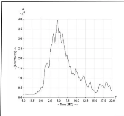
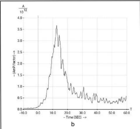
Fig. 8 shows a plot for the event 2022-01-07 17:45:34 in China. The curve of Fig. 8 is generalized parameter calculated for along the timeline in time interval sec. (Term generalized means: , where -number of used seismic records.)
This plot illustrates what was said above. There is one global pulse in general and several local pulses with small amplitudes. The graphs shown on Fig. 8 result from applying an algorithm derived from expression (8). And again, we can see one global pulse and several local pulses of sub-focuses (see Fig. 5). Fig. 5 plots were drawn along a rupture line. The Fig. 8 graph is very close to the graph on Fig. 5. The difference is in abscise units: one has a time and another depth.
The active process begins before the first braking pickup algorithm registered first arrivals. Another feature is the presence of several local maxima on both graphs. We can treat that as evidence of several focuses presented in the focal zone.
In this work, we are demonstrating the results of processing two seismic events:
- 2022-01-07 17:45:34 in China and
- 2024-01-22 18:09:09 Border of Kyrgyzstan & China.
Additional information about these events is given in Table 1.
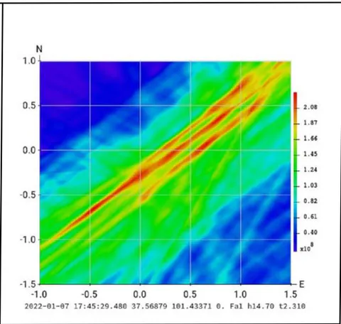
First event has a crust origin and is a moderately normal seismic event without special features. We are using it as a coaching event. Fig. 5, 8 and 9 show some abilities for analysis of evaluation of this event. Fig. 5 shows the results of location data processing. Fig. 8 presents an generalized AmP parameter in time interval sec. Fig. 9 presents a map on a horizontal slice that consists of the origin vicinity. Map demonstrates the distributions of seismic activity. It draws attention to itself that origin consists of few ruptures.
Second event has an origin depth at the bottom of crust ( ). Fig. 10.a presents the result of location data processing. It is interesting that USGS gave a depth of for both these events. It looks like this depth was fixed during the location procedure. Other features: seismic energy began to emit before first arrival times were registered (see Fig. 10.b). It is significant in seismology when we are observing some kind of precursor.
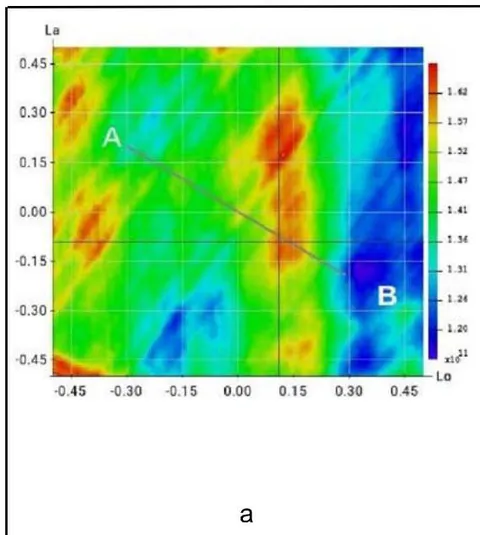
Fig. 11 presents two-dimensional slices of 3D space containing the origin. One slice Fig. 11.a presents a map of the seismic activity in the origin vicinity.
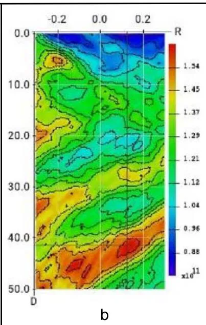
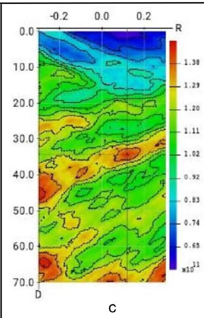
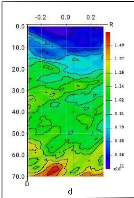
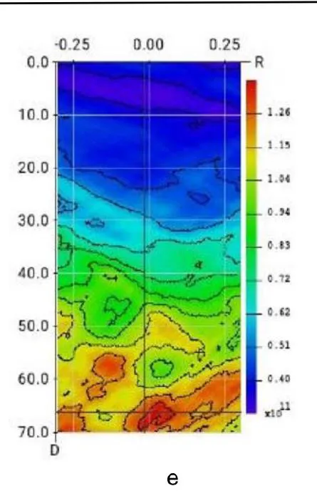
Moreover, we can trace several seconds of seismic activity before origin time on the vertical slices in coordinates in backward time perspective.. Axis is a segment of arc on the surface (line on map Fig.11. a), the unit is arc degree. Axis is depth in km. All what shows on Fig. 11 for demonstration only. It pays attention that all vertical slices correspond to times before zero time on graph Fig. 11.b. This picture series shows the rising of the seismic activity in the origin vicinity from mantle to up.
In general, Investigation of particular events does not aim for this work. It is a topic for another article.
It is required to emphasize some differences in final results of events location. Especially, strongly depends from the depth according to the rupture line properties. Coordinates have less dependents but these dependencies are present.
ACKNOWLEDGMENT
This work and investigation itself could not be successful without the help of Dr. Irina Gabsatarova and
Dr. Inessa Socolova. I express my deep appreciation to their patient, attention during our discussions and for support with data piccupping.
Seismic data was uploaded to web-services iIRIS included next seismic networks (http://ds.iris.edu/ mda): (1) II Global Seismograph Network - IRIS/IDA (Scripps Institution of Oceanography); (2) IU Global Seismograph Network IRIS/GSN (Albuquerque Seismological Laboratory/USGS).
I appreciate the ability to work for the Union Geophysical Survey of RAS. I express my appreciation to all my colleagues who help me in this long investigation.
Table 1
| Time | Location | Depth | Depth by source | M | Region & Source |
| 2022–01–07 17:45:31.832 | 37.573°N 101.435°E | 14.62 km | 13 km | 6.6 | Northern Qinghai, China. Source: USGS |
| 2024–01–22 18:09:09.223 | 41.033°N 78.905°E | 42.75 km | 13 km | 7 | Border of Kyrgyzstan & China. Source: USGS |
APPENDIX A
Coherence Level and Amplitude Parameter
Seismic records coexist with all of the seismic signals over the whole planet's crust. The difference is in amplitudes of signals. By shape all seismic signals are similar. To separate signals from different sources one can use differences in terms "similar" and "the same". It means that signal amplitudes are ignored.
Seismic signals differ by length and amplitude increasing in time. Two of these features are enough to separate different signal sources. This is used in microseismic investigations mostly. The method is based on the "comparing operator" applied to spectral phases (with unknown amplitude) of Fourier transformation of the signal's pulse. A comparing operator is applied for all available seismic records – stacking method. This may presents by expression
where - spectral phase on frequency , - weight function, - one side frequencies numbers of Fourier transformation, - number of seismic records. Algorithm is using discrete Fourier transform.
Some clarification about "one side frequency number". Obviously, the Fourier transformation is symmetrical operator in range . Fortunately there were several rules (William T. Vetterling, at. al., 1988) that permitted operation of computation to bring a simple one side numerical operator. ([Ge, M., 1995]; [Prugger, A., et al., 1989]). On the basis of it is the fact that the impulse of a seismic source is one side finite in time smooth function.
Value can be used for checking whether two or more seismic impulses coincide. It may evidence with higher degree of probability that two seismic phases and were emitted by one source. The algorithm derived from expression may operate with signals which amplitudes less than noise level.
For each seismic event frequency-time window may be determined where the coherence level reaches the maximum. Time sampling period is critical for frequency-time window parameters.
- determination of seismic depth phases pP and sP, Bull. Seism. Soc. Am., v.96, 1213-1229.
William T. Vetterling, Brian P. Flannery, William H. Press, Saul Teukolsky, (1988) Numerical Recipes, The Art of Scientific Computing, Cambridge University Press, pp.
Prugger, A. and D. Gendzwill (1989). Microearthquake location: a non-linear approach that makes use of a Simplex stepping procedure, Bull. Seism. Soc. Am. 78, pp. 799-815
Dmitry Storchak, (2011). Improved location procedures at the International Seismological Centre, Geophysical Journal International, 186, pp. 1220-1244.
The coherence is the normalized module of the complex sum of spectrum phases of the Fourier transforming of the focus impulses while spectrum amplitudes are ignored. (p.4) ↩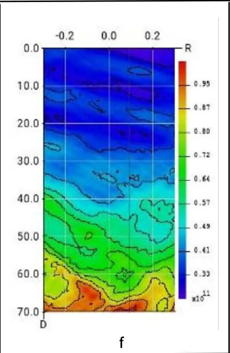
Footnotes