## I. INTRODUCTION Agriculture is the backbone of most developing countries economies, as it is a sector on which the majority of the population's livelihoods depend upon, (IPCC, 2007). Before civilization, men were surviving solely on agriculture (Amrita et al., 2017). Agriculture plays a pivotal role in the survival and existence of man, especially in SSA, where agriculture accounts for more than $75\%$ of its GDP and 70 to $80\%$ of employment (Molua and Lambi, 2007). However, environmental conditions are of vital importance in determining the amount of agricultural productivity in the region (Pimental, 2006). It is estimated that each year, approximately 10 million hectares of agrarian land globally is abandoned due to lack of production caused by environmental degradation (Lal, 1994). The situation in Sub-Saharan is more serious, as the small farmlands are located on marginal lands where soil qualities are usually poor (Lal and Stewart, 1990; David et al., 2005). However, the contribution of agricultural production to the economy of Sub-Saharan Africa over the decades is not that fixed due to the ever-changing and uncertain climate changes (David, 2005). The quantity and quality of food available in the region depend so much on climate change, as increasing rainfall, floods, drought, and sometimes extreme weather conditions influence agricultural productivity, which is the livelihood of many in the region (Amrita et al., 2017), as any change in climatic conditions will affect agricultural productivity and its nutrition outputs, (Kulkarni et al., 2018). That is why the World Food Program (WFP) in 2011 stated that environmental changes are a threat to human nature as they might increase the number of people going hungry, undernutrition, being sick, or even dying, as more powerful and frequent droughts and storms will cause more damage leading to ruining of the fertile farmlands (WFP, 2011). It is estimated therefore that, Sub-Saharan Africa by 2050 will have a drastic fall in agricultural production due to environmental changes (IPPC,2001), and this fall in agricultural production is mainly attributed to environmental degradation that has pushed many people into poverty as the majority of them depends on agriculture for their livelihood (Badulescu et al., 2019). Faced with these challenges posed by environmental degradation and other socio-economic factors on agricultural production in Sub-Saharan Africa, poverty is seen as the main factor promoting ecological degradation in the region in line with the World Commission on Environment and Development suggestion (Readon and Vosti, 1995). The nexus between environmental degradation and poverty is seen in two ways, firstly, that the poor are the source of environmental degradation and secondly they victims of a depleted environment (Oluwatoyin et al., 2018) as they are forced to cut down trees for firewood, use harmful chemicals to add their harvest and the lack of education and awareness of the effect of their practice by forgoing sustainable environmental practices for short-term benefits (Matthew et al., 2018). Also, the fact that the poor in Sub-Saharan Africa do not always have access to land, they are forced to settle in marginal land and cultivate in degraded soils, which will deplete the ground and cause more degradation of the environment (Jiang et al., 2017; and Shen et al., 2019). Based on the above trend concerning environmental degradation and agricultural productivity, the objective of this paper is to examine the nexus between ecological degradation and agrarian production in Sub-Saharan Africa and specially, to explore the effect of ecological degradation on agricultural productivity in Sub-Saharan Africa from 1996 to 2020. This paper is organised into five sections; the introduction, background, and objective made-up section 1, and the literature review is presented in section 2. Section 3 is the presentation of the methodology used in the study. The presentation of results and discussion are presented in section 4, and the conclusion and recommendation of the study are presented in section 5. ## II. LITERATURE REVIEW This part of the study centers on the conceptual issues and the empirical literature review. The section begins by explaining the essential key concepts and the conceptual framework that are relevant to this paper. The empirical literature was also reviewed, and it focuses on the previous works to provide explanations of the relationship between the various variables used in the study. ### a) Conceptual Issues Environmental degradation refers to the process by which the environment gradually gets rid of its original state, thereby reducing its biological diversity (Schubert et al., 1995). Many researchers often refer to environmental degradationas, a nontrivial and contentious concept (Todorov, 1986). The deterioration of the environment through the depletion of resources includes all biotic, and abiotic elements that form our surrounding the of the earth surface (Gascon et al., 2000). It should be noted that there are basically two main causes of environmental degradation that is human and natural activities (Wieland et al., 2020). In many parts of Sub-Saharan Africa today, there are many practices done that does not support sustainable environment (Ugochukwu, 2008). It is believed that the long-run result of environmental degradation would result in an environment that will not be able to sustain the human population, and as such, if not addressed on time, it could lead to the extinction of humanity in the future. However, in the short-run, the consequences of environmental degradation will be falling living standards, extinction of a large amount of species, decline in agricultural production amongst others. However, the contribution of agricultural production to environmental change mitigation can be through the reducing of greenhouse gas (Smith et al., 2007). CO2 is mainly released from microbial delay and sometimes from the burning of plants and organic matter and from fossil resources that are always used in agricultural production. At the same time, Methane (CH4) is produced mainly from the fermentative digestion of ruminant livestock (Mosier et al., 1998). Furthermore, Nitrous Oxide (N2O), on its part, comes from the nitrification and denitrification of nitrous (N) in the soil and manure, which usually, through its emission, leads to a higher level of nitrous fertilization (IPPC, 2007). ### b) Empirical Literature Many scientific studies have been carried in the ecosystem and its environment, especially on the effects of ecological degradation on agricultural production around the world. The nexus between environmental degradation and agricultural production has been confirmed by many studies, but the role played by poverty is still lacking in determining the strength of the relationship. However, this study bases its arguments on literature that creates a direct link between environmental degradation and agricultural production, and in this latter context that, the analysis of the role poverty plays on the relationship between environmental degradation and agrarain production in Sub-Saharan Africa is examined. In examining the relationship between environmental degradation and agricultural production, some results have stated that greenhouse gases can generate a negative effect on the agricultural value added as is observed in the results of (Muhammad et al., 2017 and Bashir et al., 2021). With this light, Musibau et al., (2021) examine the relationship between environmental degradation, energy use, and economic growth in Nigeria and arrived at a conclusion that there is an adverse association between environmental degradation and agricultural production value added. In some similar studies, Hanna et al., 2017 and Osabotrien et al., 2018 noted a similar finding to that of Chaimo and Felix, 2017 as all pointed out that environmental degradation has an adverse effect on agricultural value added. The study therefore stresses the fact that to habitat, those degraded lands for long-run development, appropriate policies and institutions, as well as enabling environment is needed to ensure that farmers participate. Hafiza et al., (2020) trying to understand the impact of average temperature, energy demand, sectorial value added and population growth on water resources quality and mortality rate in Pakistan, while using the simultaneous Generalised method of moment. The study revealed that the global average temperature has resulted in environmental problems such as the deterioration of water. This result was in line with the study of (Kocak and Sarganesi, 2017; Yildirim, 2020). The study therefore concluded by stating that the average temperature and the per capita income will reduce, while the water requirement quality and agricultural production will fall. Furthermore, Tuomisto et al., (2017) carried out a study to examine the effects of environmental changes on agriculture, nutrition, and health with their focus being on fruits and vegetables. The study argues that there is a need to develop a framework that will link the multiple interactions between environmental changes, agricultural productivity, and crop quality. Atef and Adil (2014) and Kirui et al., (2014) supported the view that there is a relationship between environmental degradation and agricultural value added and add foreign direct investment (Kim et al., 2021; Sarkodie and Strzou, 2019). Similarly, Hamdy & Aly (2014) carried out a study on land degradation, agricultural productivity, and food security. The study revealed that land properties usually decline as a result of land quality. The study stressed vital role farmers have in land degradation and the possible outcomes on agricultural productivity to boost trade openness (Karbasi and Peyravi, 2008). Dietterich et al., (2014) supported the argument that Increasing CO2 threatens human nutrition. The studies pointed to the fact that zinc and iron are the two substantial global public health problems. Gitlin et al., (2006) carried out a study on soil erosion on cropland in the United States. The study uses data from National Resource Inventory from 2003 to 2005 as the economy tries to grow in line with Smith et al., (2015). The study shows that average soil erosion rates on all cropland and the various conservation reserve program have decrease since 1982, with about $38\%$ drop. Also, Pimentel (2006) carried out research on soil erosion, a food, and environmental threat. The study stressed the fact that, soil erosion is one most serious environmental and health problem facing human beings in line with (Reangchin et al., 2019). It pointed to the fact that $99.7\%$ of the food calories of man is gotten from land and less than $0.3\%$ from the Ocean. Goodland (1997) examines the effect of environmental sustainability in agriculture; diet matters. The study emphasized on the current environmental impact on agriculture as it degrades natural capital, which is the topsoil, waste, and pollution of water, Nutrient loss and extinction of species. Similar studies, (Escribano, 2016; Chien et al., 2022) all pointed to the adverse effects on the environment in line with Rafiq et al., 2016. To conclude, from the various literature reviewed on the nexus between environmental degradation and agricultural production, it can be deduced that, in many of the studies environmental degradation harms agricultural production in Sub-Saharan Africa. However, the existing empirical literature has provided limited evidence on how poverty affects the relationship between environmental degradation and agricultural production. This study, therefore, used the opportunity to fill in the gap in the literature with special attention placed on poverty. ## III. METHODOLOGY ### a) Data Collection This study uses a panel dataset of 41 countries in Sub-Saharan Africa for the period of 25 years, which is from 1996 to 2020. The individual secondary data used in the analysis was extracted from the World Bank Development Indicator database 2020. The selection in the period, and also on the availability of data, gives justification for why we have only 41 countries in Sub-Saharan included in the study. ### b) Model Specification and Estimation Techniques To investigate the relationships between environmental degradation and agricultural production in Sub-Saharan Africa, the study adopts the empirical specification works of Altarawneh et al., 2022 with the model specified for the study as followings; $$ Y _ {i t} = A K ^ {1 - a _ {i t}} - L _ {i t} ^ {\beta}. \dots \dots \dots \dots \dots \dots \dots \dots \dots \dots \dots \dots \dots $$ Where Y is the agricultural production, K and L denote stock of environmental degradation and socio economic factors respectively. We can therefore assume that in Sub-Saharan Africa, agricultural production is closely related to the following aspects. $$ Y_{it} = (\delta_1 + ghg_{it} + FDI_{it} + IND_{it} + TOP_{it}) $$ Where, for country i at time t, AVA = Agriculture value added, GHG - Greenhouse gasses emission, FDI = Foreign Direct Investment, IND=industrialisation, TOP = Trade Openness From equation (2), if all variables can be transformed into their logarithmic form, the specification of will be; $$ ln\left(\text{AVA}\right)_{\mathrm{it}} = \Theta + \beta_{1\mathrm{t}} \text{Inghg}_{\mathrm{it}} + \beta_{2\mathrm{t}} \text{InFDI}_{\mathrm{it}} + \beta_{3\mathrm{t}} \text{Ind}_{\mathrm{it}} + \beta_{4\\mathrm{t}} \text{InTOP}_{\mathrm{it}} + U_{\mathrm{it}}. $$ We used the Pooled Mean Group Estimator (PMGE) to analyses our dataset. The PMGE is also known the Maximum Likelihood (ML). This estimation technique was formulated by Newton-Raphson. The technique allows for the short-run parameters to differ between groups but imposing it equality in the long term coefficient between the same groups. ## IV. PRESENTATION AND DISCUSSION OF RESULTS ### a) Descriptive Statistics Table 1 presents the summary of the descriptive statistics of the variables of this paper between the periods 1996 to 2020. A total of 1025 observations were considered. This means that the number of years in which a particular variable has been used (25 years) and multiple by the number of countries (41). Table 1, therefore, shows the different facts about the data, such as the mean, standard deviation, and the minimum and maximum values. Table 1: Summary of the Descriptive Statistics <table><tr><td>Variable</td><td></td><td>Mean</td><td>Std. Dev.</td><td>Min</td><td>Max</td><td>Observations</td></tr><tr><td rowspan="3">Ava</td><td>Overall</td><td>21.78563</td><td>14.09931</td><td>.8926961</td><td>61.41626</td><td>N = 1025</td></tr><tr><td>Between</td><td></td><td>13.59743</td><td>1.73529</td><td>53.43239</td><td>n = 41</td></tr><tr><td>Within</td><td></td><td>4.270109</td><td>-.5312841</td><td>48.19511</td><td>T = 25</td></tr><tr><td rowspan="3">Lnghg</td><td>Overall</td><td>9.634087</td><td>1.462704</td><td>5.703783</td><td>12.64899</td><td>N = 943</td></tr><tr><td>Between</td><td></td><td>1.460705</td><td>6.007065</td><td>12.36611</td><td>n = 41</td></tr><tr><td>Within</td><td></td><td>.2359578</td><td>8.052291</td><td>10.22524</td><td>T = 23</td></tr><tr><td rowspan="3">Ind</td><td>Overall</td><td>25.60674</td><td>12.81537</td><td>4.555926</td><td>84.3492</td><td>N = 1002</td></tr><tr><td>Between</td><td></td><td>12.66929</td><td>11.36161</td><td>68.03252</td><td>n = 41</td></tr><tr><td>Within</td><td></td><td>4.671993</td><td>-.233834</td><td>57.0531</td><td>T-bar = 24.439</td></tr><tr><td rowspan="3">Fdi</td><td>Overall</td><td>4.079865</td><td>8.101796</td><td>-11.19897</td><td>161.8237</td><td>N = 1025</td></tr><tr><td>Between</td><td></td><td>3.828416</td><td>.4613821</td><td>19.46647</td><td>n = 41</td></tr><tr><td>Within</td><td></td><td>7.164206</td><td>-19.40623</td><td>146.4371</td><td>T = 25</td></tr><tr><td rowspan="3">Top</td><td>Overall</td><td>69.21001</td><td>34.78102</td><td>.7846308</td><td>225.0231</td><td>N = 1003</td></tr><tr><td>Between</td><td></td><td>32.59774</td><td>21.81432</td><td>169.9495</td><td>n = 41</td></tr><tr><td>Within</td><td></td><td>15.16375</td><td>-20.1498</td><td>128.4365</td><td>T-bar = 24.4634</td></tr></table> The study reveals that the mean value of agricultural value added in Sub-Saharan Africa is 21.8, while the minimum value is 0.89 and the maximum value stood at 61.4. The standard deviation for agricultural value added within sub-Saharan Africa for 25 years was 14.1. Meanwhile, between the countries in Sub-Saharan Africa, the maximum value recorded was $53.43\%$ and a minimum value of 1.7 with a standard deviation of 13.6. However, within the countries in the region, the minimum value stood at -0.53, and the maximum value was 48.2 with a standard deviation of $4.3\%$. Statistics on agricultural value-added shows that the total number of observations $N = 1025$ and the number of countries involved in study $n = 41$ within the period (T) of 25 years. The statistics show that greenhouse gasses emission on average was 9.6 in Sub-Saharan Africa within the period of the study. The maximum value recorded was 12.6, while the minimum value was 5.7 with a standard deviation of $1.4\%$. However, statistics within Sub-Saharan African countries show that the greenhouse gases emission minimum value was 8.1 while the maximum value was 10.2, and a standard deviation within the region stood at 0.23. On the other hand, the values between the Sub-Saharan African countries indicate that the maximum value was 12.4, and the minimum value is $6\%$ with a standard deviation of 1.5. Thus, greenhouse gas emission records that the total number of observations $N = 943$ for $n = 41$ countries in the region within a period $T = 23$ years. Furthermore, the mean value of industrialisation in Sub-Saharan Africa within the study period (25 years) was 25.61. The minimum value in the region was 4.6, and the maximum value was $84.3\%$, with a standard deviation of 12.8. On the other hand, statistics between the countries in the area indicate that the minimum value is 11.4, and the maximum value is $68.03\%$, with the standard deviation between the countries being 12.7. However, the value within sub-Saharan African shows that the minimum value is $-0.23\%$, and 57.1 was recorded for the maximum value, with the standard deviation within the region being 4.7. The records show that within $(T) = 24$ years, $N = 1002$ observations were considered for $n = 41$ countries. In addition, Foreign Direct Investment in Sub-Saharan Africa had an average value of 8.1. The maximum value for the region was 161.8, and the minimum value stood at 11.2 with a standard deviation of $8.1\%$. Statistics within the Sub-Saharan shows that, the maximum value stood at 146.4 while the minimum value for the region within the countries is $-19.4\%$ with a standard deviation of 7.2. On the other hand, the value between the Sub-Saharan Africa show that the minimum value is 0.46 and the maximum value is 19.5 with a standard deviation of $3.8\%$. The result record that 1025 observations were involved, (N) in 41 countries, (n) within the time lag (T) of 25 years Finally, statistics on Trade openness show that the mean value stood at 69.2 in Sub-Saharan Africa. While the minimum value recorded within the same period was $0.78\%$, and the maximum value stood at 255 with a standard deviation of $34.9\%$. However, statistics between Sub-Saharan African countries show that the maximum is 169.9, and the minimum value is 21.85 with a standard deviation of 32.6. On the other hand, the values within the region indicate that the maximum value is 128, and the minimum value is -20 with a standard deviation of $15.2\%$. The results considered 1003 observations (N) for 41 countries (n) within the time lag of 24 years. ### b) Correlation Analysis In order to measure, the degree of relationship existing between variables, a correlation analysis was performed. Table 2 provides the correlation matrix of residuals between different variables used in environmental degradation and agricultural productivity. Table 2: Correlation Matrix of Residuals <table><tr><td></td><td>Ava</td><td>Lnghg</td><td>Ind</td><td>Fdi</td><td>Top</td></tr><tr><td>Ava</td><td>1.0000</td><td></td><td></td><td></td><td></td></tr><tr><td>Lnghg</td><td>0.1260</td><td>1.0000</td><td></td><td></td><td></td></tr><tr><td></td><td>(0.0001)</td><td></td><td></td><td></td><td></td></tr><tr><td>Ind</td><td>-0.5991</td><td>0.1176</td><td>1.0000</td><td></td><td></td></tr><tr><td></td><td>(0.0000)</td><td>(0.0004)</td><td></td><td></td><td></td></tr><tr><td>Fdi</td><td>-0.1475</td><td>-0.0839</td><td>0.0909</td><td>1.0000</td><td></td></tr><tr><td></td><td>(0.0000)</td><td>(0.0100)</td><td>(0.0040)</td><td></td><td></td></tr><tr><td>Top</td><td>-0.5549</td><td>-0.3598</td><td>0.4274</td><td>0.3942</td><td>1.0000</td></tr><tr><td></td><td>(0.0000)</td><td>(0.0000)</td><td>(0.0000)</td><td>(0.0000)</td><td></td></tr></table> ## i. Stationary Test Results To check for the stationary of the results, the paper employed the Im-Pesaran-Shin unit root test. The results are presented in table A in the appendix. The results from the Im-Pesaran-Shin unit root indicate that only FDI was stationary at the level, and it was after the first difference that other variables obtained their stationarity. ## ii. The Scatter Diagram This scatter diagram reveals the coefficients' direction, strength, and how linear agricultural value added and greenhouse gases emission are. It aids in explaining the existing relationship between agricultural value added and greenhouse gas emissions. The X-axis represents the independent variable (greenhouse gas emission), while the Y-axis stands for the dependent variable (agriculture value added). 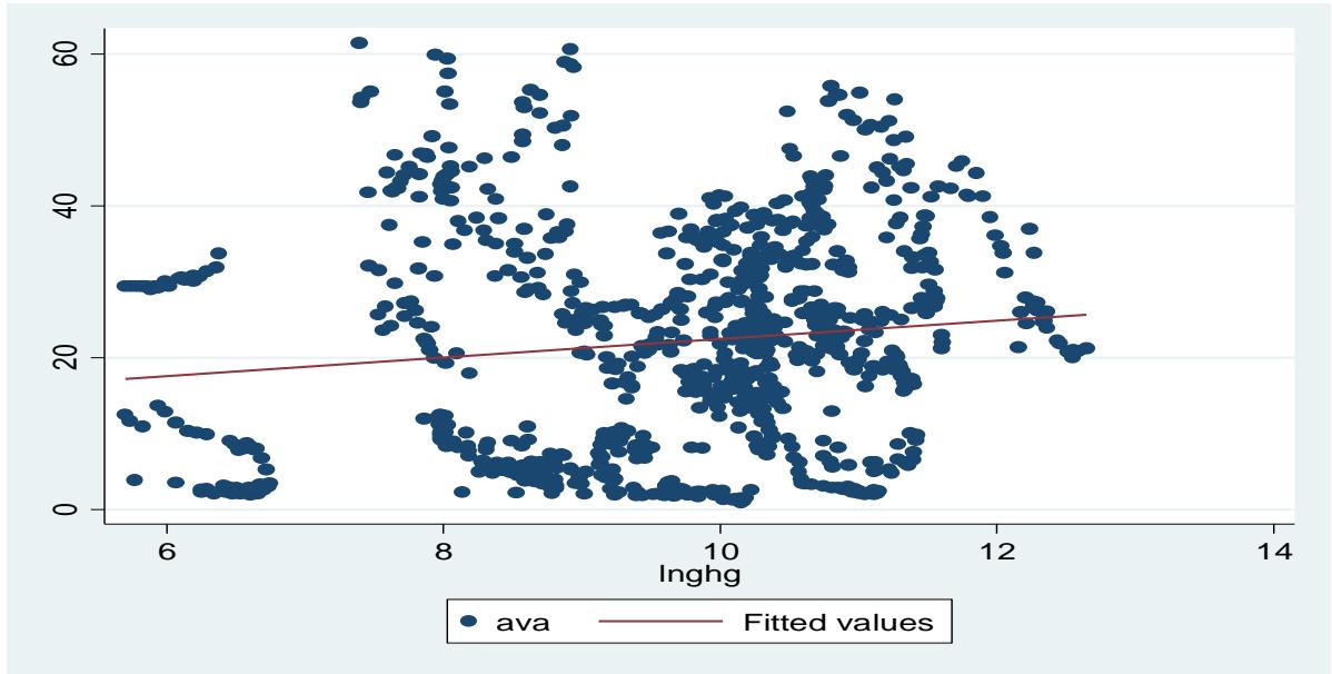 Figure 1: Scatter diagram of AVA and GHG Source: Composed by Researcher using STATA (version 14) The diagram explains that the two variables can either be positive or negative depending on the direction of each other. The positive relationship between agriculture value added and greenhouse gas emission means that all the variables are increasing. Meanwhile, a negative long-run relationship means that as greenhouse gas emission increase and agricultural value added is reduced. Furthermore, when greenhouse gas emission is between 6-8, the rate at which they are scattered is high. This means that the strength between the two variables (GHG and AVA) is not strong as compared to when the GHG is at 10. The rate of cluster around the fitted line value is tighter, showing a stronger relationship. In addition, the diagram indicates that the relationship existing between agricultural value added and greenhouse gas emission is linear, as this linearity is shown in the fitted line inside the scatter diagram. ## iii. Regression Results Table 3 presents the results of Pooled mean Group estimation results. Table 3: Pooled Mean Group (PMG) <table><tr><td>METHODS</td><td>PMGE</td><td></td></tr><tr><td></td><td>Coefficient (Standard error) SR</td><td>Coefficient (Standard error) Ec (LR)</td></tr><tr><td>EC</td><td>-0.176***</td><td></td></tr><tr><td></td><td>(0.0413)</td><td></td></tr><tr><td>Lnghg</td><td>-1.800</td><td>2.313***</td></tr><tr><td></td><td>(2.022)</td><td>(0.521)</td></tr><tr><td>Ind</td><td>-0.209**</td><td>-1.104***</td></tr><tr><td></td><td>(0.0815)</td><td>(0.0476)</td></tr><tr><td>Fdi</td><td>-0.0117</td><td>0.342***</td></tr><tr><td></td><td>(0.0642)</td><td>(0.0823)</td></tr><tr><td>Top</td><td>0.0145</td><td>-0.0617**</td></tr><tr><td></td><td>(0.0194)</td><td>(0.0298)</td></tr><tr><td>Constant</td><td>5.704***</td><td></td></tr><tr><td></td><td>(1.489)</td><td></td></tr><tr><td>Observations</td><td>868</td><td>868</td></tr></table> The results show that the coefficient of greenhouse gas is negative indicating that an increase in greenhouse gas emission will lead to decrease in agriculture value added. In quantitative terms, the results, the result shows that a 1 percent increase in greenhouse gas will leads to 1.8 percent decrease in agricultural value added in the short-run. In the long-run, an increase in greenhouse gas will leads to an increase agricultural value added. That is a 1 percent increase in greenhouse gas will leads to 2.313 percent increase in agricultural value added. This result is statistically significant at 1 percent level of significance. The result is in line with the result of Muhammad et al., (2017), although in contrast to those of (Hanna et al., 2017; Osabotrien et al., 2018 and Chaimo and Felix, 2017). The result gives the impression that an increased in the greenhouse gases in Sub-Saharan Africa will lead to an increase in agricultural value added in the long-run as compared to when the greenhouse gases are low. This is better explained by the fact that greenhouse gases have a positive impact on some particular crop production. Also the coefficient of industrialisation is negative and statistically significant for both the short and long-run, although with differences in the magnitude of the coefficient. This negative coefficient shows that an increase in industrialisation will lead to a decrease in agricultural value added. In the short-run, an increase in industrialisation by 1 percent will lead to a decrease of 0.209 percent of agricultural value added and in the long-run, 1 percent increase in industrialisation will lead to a decrease of 1.104 percent of agricultural value added. The result is in line with the result of Dodzin, S., & Vamvakidis, A. (2004). This meaning that countries in Sub-Saharan with higher industrialisation will likely witness a decrease in their agriculture value added. Furthermore, the result from Foreign Direct Investment (FDI) in the short-run reveals that $1\%$ increase in foreign direct investment in Sub-Saharan Africa will lead to a decrease in agricultural value added by approximately $0.0117\%$ considering the fact that, all other determinants affecting agricultural value added are held constant. This coefficient is statistically significant at $5\%$ level of significance. In the long-run, 1 percent increase in foreign direct investment will lead to an increase in agricultural value added by 0.342 and the result is significant at 1 percent level of significance. The result is in line with (Kumar and Gopalsamy, 2019; Musibau et al., 2021 and Kim et al., 2021 which also indicated a positive relationship between foreign direct investment and agricultural value added. This means that an improvement in FDI will lead to a rise in agricultural value added, and the reduction in it will lead to a fall in agricultural value added. Similarly, trade openness result reveals that a $1\%$ increase in trade openness will leads an approximately $0.014\%$ increase in agriculture value added in the short-run. In the long-run, 1 percent increase in trade openness will lead to a decrease in agricultural value added by 0.0617 and it is significant at 5 percent level of significance. This result is significant at a $1\%$ level of significance. The result is in line with Rafiq et al., 2016 although in contrast to the finding of Karbasi and Peyravi 2008 in Iran. The result gives the impression that when trade openness in Sub-Saharan Africa increase, agriculture value added always falls. Lastly, the constant shows that, even without any variable mentioned in the model, agriculture value added will still increase by 5.704 percent. This value is statistically significant at the 5 level of significance. Without any coefficient affecting agriculture value-added, there will still be an increase of approximately $5.704\%$. The error correction (ECM) makes it possible to handle non-stationary data series and to separates the long and short run. The error correction is -0.176 and significant at 1 percent, shows the presence of a long-run causal relationship between variables. ## V. CONCLUSION AND POLICY IMPLICATIONS This paper examined the relationship between environmental degradation and agricultural production in Sub-Saharan Africa. It adopted a mixed research design, as it uses both descriptive and evaluative research design, and the pooled mean group estimation technique was used to analyse the dataset for SSA. The finding revealed that greenhouse gas has a positive effect on agricultural value added in the long-run and in the short-run has a negative effect in Sub-Saharan Africa. This paper concludes by recommending that various agents should encourage the use of organic manure rather than chemicals that usually degrade the environment, farms lands should be equitably distributed among the poor farmers, and that agricultural production should not be practiced in marginal lands. Concerning the scope for further studies, this article recommends that the aspect of the culture of the people should be incorporated when examining the relationship between environmental degradation and agricultural productivity in Sub-Saharan Africa. ### APPENDIX Table: Summary of Im-Pesaran-Shin Unit-Root Test of Stationarity <table><tr><td>Variables</td><td>Test Statistics at Levels</td><td>Critical Values at 5% and P-Values</td><td>Test Statistics After First Difference</td><td>Critical Value at 5%</td><td>Decision</td></tr><tr><td>AVA</td><td>-1.2868</td><td>-1.730P=0.0991</td><td>-16.1940</td><td>-1.730P=0.000</td><td>I (1)</td></tr><tr><td>Inghg</td><td>2.9108</td><td>-1.730P=0.9982</td><td>-14.4412</td><td>-1.730P=0.000</td><td>I (1)</td></tr><tr><td>Ind</td><td>0.5088</td><td>-1.730P=0.3054</td><td>-15.3103</td><td>-1.730P=0.000</td><td>I (1)</td></tr><tr><td>FDI</td><td>-9.0349</td><td>-1.730P=0.000</td><td></td><td></td><td>I (0)</td></tr><tr><td>TOP</td><td>-1.1509</td><td>-1.730P=0.1249</td><td>15.70691</td><td>-1.730P=0.000</td><td>I (1)</td></tr><tr><td>Variables</td><td>Test statistics at levels</td><td>Critical values at 5% and P-values</td><td>Test statistics after first difference</td><td>Critical value at 5%</td><td>Decision</td></tr><tr><td>AVA</td><td>-1.2868</td><td>-1.730P=0.0991</td><td>-16.1940</td><td>-1.730P=0.000</td><td>I (1)</td></tr><tr><td>Inghg</td><td>2.9108</td><td>-1.730P=0.9982</td><td>-14.4412</td><td>1.730P=0.000</td><td>I (1)</td></tr><tr><td>Ind</td><td>0.5088</td><td>-1.730P=0.3054</td><td>-15.3103</td><td>-1.730P=0.000</td><td>I (1)</td></tr><tr><td>FDI</td><td>-9.0349</td><td>-1.730P=0.000</td><td></td><td colspan="2">I (0)</td></tr><tr><td>TOP</td><td>-1.1509</td><td>-1.730P=0.1249</td><td>15.70691</td><td>-1.730P=0.000</td><td>I (1)</td></tr></table>

Generating HTML Viewer...

References

39 Cites in Article
M Amrita Sujlana,B Parampreetpannu,Japneet (2017). Double mesiosens: a rewiew and report of 2 cases.
Heba Altarawneh,Hiam Chemaitelly,Houssein Ayoub,Patrick Tang,Mohammad Hasan,Hadi Yassine,Hebah Al-Khatib,Maria Smatti,Peter Coyle,Zaina Al-Kanaani,Einas Al-Kuwari,Andrew Jeremijenko,Anvar Kaleeckal,Ali Latif,Riyazuddin Shaik,Hanan Abdul-Rahim,Gheyath Nasrallah,Mohamed Al-Kuwari,Adeel Butt,Hamad Al-Romaihi,Mohamed Al-Thani,Abdullatif Al-Khal,Roberto Bertollini,Laith Abu-Raddad (2022). Effect of prior infection, vaccination, and hybrid immunity against symptomatic BA.1 and BA.2 Omicron infections and severe COVID-19 in Qatar.
Adil Atef (2014). Land Degradation, Agriculture Productivity and Food Security.
Daniel Badulescu,Ramona Simut,Alina Badulescu,Andrei-Vlad Badulescu (2019). The Relative Effects of Economic Growth, Environmental Pollution and Non-Communicable Diseases on Health Expenditures in European Union Countries.
M Bashir,B Sheng,M Farooq,M Bashir,U Shahzad (2021). The role of macroeconomic and institutional factors in foreign direct investment and economic growth: empirical evidence in the context of emerging economies.
F Chien,C Hsu,I Ozturk,A Sharif,M Sadiq (2022). The role of renewable energy and urbanization towards greenhouse gas emission in top Asian countries: Evidence from advance panel estimations.
O Chioma,Felix (2017). Evaluation of the contemporary issues in data Mining and data Warehousing.
Dunn David,Stevens Gene,Kendig Andy (2005). Boron Fertilization of Rice with Soil and Foliar Applications.
L Dietterich,A Zanobetti,I Kloog,P Huybers,A Leakey,A Bloom,. Myers,S (2014). Increasing CO2 threatens human nutrition.
S Dodzin,A Vamvakidis (2004). Trade and industrialization in developing economies.
Alfredo Escribano (2016). Organic Livestock Farming — Challenges, Perspectives, and Strategies to Increase Its Contribution to the Agrifood System’s Sustainability — A Review.
P Konvalina (1980). Biology.
Claude Gascon,Jay Malcolm,James Patton,Maria Da Silva,James Bogart,Stephen Lougheed,Carlos Peres,Selvino Neckel,Peter Boag (2000). Riverine barriers and the geographic distribution of Amazonian species.
Alicyn Gitlin,Christopher Sthultz,Matthew Bowker,Stacy Stumpf,Kristina Paxton,Karla Kennedy,Axhel Muñoz,Joseph Bailey,Thomas Whitham (2006). Mortality Gradients within and among Dominant Plant Populations as Barometers of Ecosystem Change During Extreme Drought.
R Goodland (1997). Environmental sustainability in agriculture: diet matters.
Hafiza Tehreem,Muhammad Anser,Abdelmohsen Nassani,Muhammad Abro,Khalid Zaman (2020). Impact of average temperature, energy demand, sectoral value added, and population growth on water resource quality and mortality rate: it is time to stop waiting around.
A Hamdy,A Aly (2014). Land degradation, agriculture productivity and food security.
Hanna (2001). Effects of environmental change on agriculture, nutrition and health: A framework with a focus on fruits and vegetables.
Abdul Jalil,Abdul Rauf,Waqas Sikander,Zhang Yonghong,Wang Tiebang (2021). Energy consumption, economic growth, and environmental sustainability challenges for Belt and Road countries: a fresh insight from “Chinese Going Global Strategy”.
F Jiang,Y Jiang,H Zhi,Y Dong,H Li,S Ma,. Wang,Y (2017). Artificial intelligence in healthcare: past, present and future.
A Karbasi,M Peyravi (2008). Effect of Trade Openness on Agricultural Value Added in Iran.
Sunghwan Kim,Jie Chen,Tiejun Cheng,Asta Gindulyte,Jia He,Siqian He,Qingliang Li,Benjamin Shoemaker,Paul Thiessen,Bo Yu,Leonid Zaslavsky,Jian Zhang,Evan Bolton (2021). PubChem in 2021: new data content and improved web interfaces.
Oliver Kirui (2014). Economics of Land Degradation and Improvement in Tanzania and Malawi.
Emrah Koçak,Aykut Şarkgüneşi (2017). The renewable energy and economic growth nexus in Black Sea and Balkan countries.
Shruti Kulkarni,Shah Mandal,G Sharma,Monica Mundada,Meeradevi (2018). Predictive Analysis to Improve Crop Yield using a Neural Network Model.
M Kumar,S Gopalsamy (2019). Agricultural sector FDI and economic growth in SAARC countries.
R Lal (1994). Soil erosion research methods.
Oluwatoyin Matthew,Oluwarotimi Owolabi,Romanus Osabohien,Ese Urhie,Toun Ogunbiyi,Tomike Olawande,Oluwatosin Edafe,Praise Daramola (2020). CARBON EMISSIONS, AGRICULTURAL OUTPUT AND LIFE EXPECTANCY IN WEST AFRICA.
O Matthew,R Osabohien,F Fasina,A Fasina (2018). Greenhouse gas emissions and health outcomes in Nigeria: Empirical insight from ARDL technique.
Ernest Molua,Cornelius Lambi (2007). The Economic Impact Of Climate Change On Agriculture In Cameroon, Volume 1of 1.
Arvin Mosier,Carolien Kroeze,Cindy Nevison,Oene Oenema,Sybil Seitzinger,Oswald Van Cleemput (1998). Closing the global N2O budget: nitrous oxide emissions through the agricultural nitrogen cycle.
Hassan Muhammad,Thomas Fuchs,Nicole De Cuir,Carlos De Moraes,Dana Blumberg,Jeffrey Liebmann,Robert Ritch,Donald Hood (2017). Hybrid Deep Learning on Single Wide-field Optical Coherence tomography Scans Accurately Classifies Glaucoma Suspects.
Hammed Musibau,Waliu Shittu,Fatai Ogunlana (2021). The relationship between environmental degradation, energy use and economic growth in Nigeria: new evidence from non-linear ARDL.
A Oluwatoyin,A Oluwarotimi,Owolabi1,O Romanus,U Ese,O Toun,Tomike Olawande,D Oluwatosin,Edafe,J Praise,Daramola (2018). Carbon Emissions, Agricultural Output and Life Expectancy in West Africa.
Romanus Osabohien,Evans Osabuohien,Ese Urhie (2018). Food Security, Institutional Framework and Technology: Examining the Nexus in Nigeria Using ARDL Approach.
D Pimental (2006). Soil Erosion: A Food and Environmental Threat.
Shuddhasattwa Rafiq,Ruhul Salim,Ingrid Nielsen (2016). Urbanization, openness, emissions, and energy intensity: A study of increasingly urbanized emerging economies.
Thomas Reardon,Stephen Vosti (1995). Links between rural poverty and the environment in developing countries: Asset categories and investment poverty.
Promporn Reangchim,Tinnakorn Saelee,Vorranutch Itthibenchapong,Anchalee Junkaew,Narong Chanlek,Apiluck Eiad-Ua,Nawee Kungwan,Kajornsak Faungnawakij (2019). Role of Sn promoter in Ni/Al<sub>2</sub>O<sub>3</sub> catalyst for the deoxygenation of stearic acid and coke formation: experimental and theoretical studies.
No ethics committee approval was required for this article type.
Data Availability
Not applicable for this article.
How to Cite This Article
Menang Etiene Fomonyuy. 2026. \u201cNexus between Environmental Degradation and Agricultural Productivity in sub Sahara Africa; does Poverty Matters?\u201d. Global Journal of Management and Business Research - B: Economic & Commerce GJMBR-B Volume 23 (GJMBR Volume 23 Issue B2).
Explore published articles in an immersive Augmented Reality environment. Our platform converts research papers into interactive 3D books, allowing readers to view and interact with content using AR and VR compatible devices.
Your published article is automatically converted into a realistic 3D book. Flip through pages and read research papers in a more engaging and interactive format.
Our website is actively being updated, and changes may occur frequently. Please clear your browser cache if needed. For feedback or error reporting, please email [email protected]
Thank you for connecting with us. We will respond to you shortly.