On the Generalized Power Transformation of left Truncated Normal Distribution

Okoli Christian O.; Nwosu Dozie F.; Osuji George A.; Nsiegbe A.

I. INTRODUCTION AND PRELIMINARY

Let $\omega$ be an element of an appropriate non-empty sample space $\Omega$ and $X\colon \Omega \longrightarrow \mathrm{R}(R = (-\infty,\infty))$ a real-valued function (random variable) defined on $\Omega$ . To each element of the event

is associated with a probability measure $P:2^{\Omega}\to[0,1]$ in the measure space $(\Omega,2^{\Omega},P)$ and then denotes the probability density function (pdf) f associated with the real-valued function (random variable) X by $f(x)$ . Where $f:X(\Omega)\to[0,1]$ .

Let $\alpha$ be an arbitrary but fixed point of a scalar field $\mathcal{F}$ ( $i.e.\alpha\in\mathcal{F}$ ), then we consider a continuous bijective function or transformation $h_{\alpha}:X(\Omega)\to\mathrm{R}$ define by

If $f_{h_{\alpha}}$ is the function induced by $h_{\alpha}$ on f, then we denoted the probability density function (pdf) g associated with the real-valued function (random variable) $h_{\alpha}$ by $f_{h_{\alpha}}(x)$ ; $f_{h_{\alpha}}$ is the probability density function induced by $h_{\alpha}$ on f such that

Remark 1.1

If $\alpha = 0$ , then $h_{\alpha}$ (i.e. $h_0$ ) reduces to a constant function. Hence at this point the domain of $g$ reduces to a singleton set which is not of interest (in terms of data transformations).
If $\alpha = 1$ , then $h_{\alpha}$ (i.e. $h_1$ ) reduces to a identity function so that $g(x) = f(x)\forall x\in$ $\mathrm{X}(\Omega)$ .

Hence in this research, we require that $\alpha \neq 0$ , as such we consider the following propositions:

Proposition 1.2 If $\alpha \leq -1$ , then $g$ is an inverse $\alpha$ -power transform of $f$ . Proof.

This easily follows from the fact that $h_{\alpha}(x) = \frac{1}{x^{\alpha}} \forall \alpha \geq 1$ .

Notes

Proposition 1.3 If $\alpha \geq 1$ , then $g$ is an $\alpha$ -power transform of $f$ .

Proof.

This easily follows from the fact that $h_{\alpha}(x) = x^{\alpha} \quad \forall \alpha \geq 1$ .

Proposition 1.4 If $0 < \alpha < 1$ , then there exist a positive constant $c$ such that $g$ is a $(c + 1)$ th root power transform of $f$ .

Proof.

If $0 < \alpha < 1$ , then it follows that $\frac{1}{\alpha} > 1; \Longrightarrow \frac{1}{\alpha} = 1 + c$ , for some $c > 0$ ;

$\Rightarrow \alpha = \frac{1}{1 + c}$ , for some $c > 0$ , so that $h_\alpha(x) = x^{\frac{1}{1 + c}} \forall c > 0$ which is as stated.

Proposition 1.5 If $-1 < \alpha < 0$ , then there exist a positive constant c such that g is an inverse $(c + 1)$ th root power transform of f.

Proof.

If $-1 < \alpha < 0$ , then it follows that $0 < -\alpha < 1; \Rightarrow 0 < \beta < 1$ , where $\beta = -\alpha$ . Thus by proposition 1.4 $\beta = \frac{1}{1 + c}$ , for some $c > 0$ ;

$\Rightarrow \alpha = \frac{-1}{1 + c}$ , for some $c > 0$ which is as stated.

Remark 1.6

Now, observe in particular;

In proposition 1.2, if $\alpha = -1, -2$ , then $g$ is an inverse, inverse square, transform of $f$ respectively.
In proposition 1.3, if $\alpha = 1,2$ , then $g$ is the identity, square, transform of $f$ respectively.
In proposition 1.4, if $c = 1, \Rightarrow \alpha = \frac{1}{2}$ , then $g$ is a square root transform of $f$ .
In proposition 1.5, if $c = 1, \Rightarrow \alpha = -\frac{1}{2}$ , then $g$ is an inverse square root transform of $f$ .

II. THE LEFT TRUNCATED NORMAL DISTRIBUTION

Definition 2.1 Let X be a random variable that follows a normal distribution with $\mu(\mu \neq 0)$ and variance $\sigma^{2}(\sigma^{2} > 0)$ (i.e. $X \sim (\mu, \sigma^{2})$ ) then the probability distribution function (pdf)[4] is given by

Ref

Lifetime data pertain to the lifetimes of units, either industrial or biological, an industrial or a biological unit cannot be in operation forever. Such a unit cannot continue to operate in the same condition forever. Any random variable is said to be truncated if it can be observed over part of its range. Truncation occurs in various situations. For example, right truncation occurs in the study of life testing and reliability of items such as an electronic component, light bulbs, etc. Left truncation arises because, in many situations, failure of a unit is observed only if it fails after a certain period (for more on this, see $[14-15]$ and the references therein). Unfortunately, often time in practice, the random variable X which follows a $N(\mu,\sigma^{2})$ distribution do not take values that are less than or equal to zero ( $X \leq 0$ ). As such, it naturally calls for one to truncate the pdf in (2.1) to take care of the restriction of the random variable in the region $X \wr 0$ without alteration to the properties of the pdf. Hence we seek for such truncated normal distribution of f and then denote it by $f_{T}$ . It suffices to find a constant M such that $\int_{0}^{\infty} Mf(x)dx = 1$ , where M is the so-called normalizing constant and then define $f_{T}(x) = Mf(x)$ .

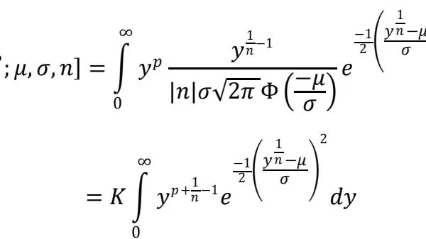
Now, we solve for such $M$ by evaluating the integral $\int_0^\infty f(x)dx$ . Observe that if we take $z = \frac{x - \mu}{\sigma}$ , then

It then follows that $M = \frac{1}{\Phi\left(\frac{-\mu}{\sigma}\right)}$ . Hence, the left truncated normal distribution of f is given by

Observe that $0 \leq f_{T}(x; \mu, \sigma) \leq 1$ $\forall x \in R_{+}$ ( $R_{+} = (0, \infty)$ ) and by the method of derivation of $f_{T}(x; \mu, \sigma)$ , we have that $\int_{0}^{\infty} f_{T}(x; \mu, \sigma) dx = 1$ . Thus $f_{T}(x; \mu, \sigma)$ is a proper pdf.

III. DISTRIBUTION ASSOCIATED WITH TRUNCATED NORMAL DISTRIBUTION UNDER ARBITRARY $\alpha$ -POWER TRANSFORMATION

Let $\alpha$ be an arbitrary but fixed point of a scalar field $\mathcal{F}$ ( $i.e.\alpha\in\mathcal{F}$ ) and $h_{\alpha}(x)=x^{\alpha}$ . $\forall\alpha\in\mathcal{F}$ as in equation (1.2). There is no loss of generality if we put $y=h_{\alpha}(x)$ and $\alpha=n$ ; $\Rightarrow y=x^{n}$ . Hence by standard result in classical calculus [2], the transformed function $g$ induced by $h_{\alpha}$ on $f$ is given by

Where $\left|\left|\frac{dx}{dy}\right|\right|$ is the absolute value of the Jacobian (determinant) of the transformation [2]. If $y = x^{n}$ , then

By substituting appropriately into equation (3.1) and simplifying, we have

Notes otherwise

It now remain to show that $g(y; \mu, \sigma, n)$ given in equation (3.2) is a well-defined pdf. It suffices to show that $\int_0^\infty g(y; \mu, \sigma, n) dy = 1$ . To see this we proceed as follows:

Let $u = y^{\frac{1}{n}}$ ; $\Rightarrow dy = n y^{1 - \frac{1}{n}}$ du, substituting into the integral above gives

Let $z = \frac{u - \mu}{\sigma}$ ; $\Rightarrow \sigma dz = du$ , substituting into the integral above gives

This is as required.

IV. THE jth MOMENT ABOUT THE MEAN AND THE ORIGIN

In this section, for all fixed $n \in R$ , we solved for the jth moment of the random variable Y about the mean $\mu$ , which is also called the jth central moment is defined as $\mu_{j}(\mu, \sigma, n) = E[(Y - \mu)^{j}; \mu, \sigma, n](\mu_{j}(n) \text{ for short})$ . This implies that

Ref

and we proceed to compute the pth moment about the origin $E[Y^{P};\mu,\sigma,n]$ which is given by

Let $u = y^{\frac{1}{n}}$ ; $\Rightarrow dy = ny^{1 - \frac{1}{n}}$ du, substituting into the integral above and simplifying, we have

Observe that the series $\sum_{r\geq 0}\frac{\left(\frac{u}{\sigma^2}\right)^r}{r!}$ converges uniformly (by ratio test) [3,13], hence by Taylors series expansion, for some positive constant $k$ (sufficiently large enough) [3,13], there exists a number $\delta (r_k)$ between 0 and $\frac{u}{\sigma^2}$ such that $\delta (r_k)\to 0$ as $r\rightarrow \infty$ , it then follows that as $r\longrightarrow \infty$

Let $w = \frac{u^2}{2\sigma^2}$ ; $\Rightarrow \sigma^2 dw = u du$ , then substituting appropriately into the integral above and simplifying, we have

Thus,

Ref

And

Where $\lfloor x\rfloor$ is the greatest integer function less than x.

It is important to observe that in particular, in equation (4.2), if we take n = -1, then g is an inverse transform of f and by putting k = 7, $\mu = 1$ and evaluating $E[Y^{P}; 1, \sigma, -1]$ at p = 1, 2 respectively, we obtain the result in [6].

Remark 4.1 Further more observe that;

Iwueze (2007), for $\mu = 1$ , $n = 1$ , the authors expressed $E[Y]$ in terms of cumulative distribution function of the standard normal distribution and $E[(Y - 1)^2]$ in terms of cumulative distribution function of the standard normal distribution and Chi-square distribution function,

Ref

Nwosu, Iwueze and Ohakwe (2010), for $\mu = 1, n = -1$ , the authors expressed $E[Y]$ and $E[(Y - 1)^{2}]$ in terms of cumulative distribution function of the standard normal distribution and Gamma distribution function,
Ohakwe, Dike and Akpanta (2012), for $\mu = 1, n = 2$ , the authors expressed $E[Y]$ and $E[(Y - 1)^{2}]$ in terms of cumulative distribution function of the standard normal distribution,
Nwosu, Iwueze, and Ohakwe. (2013), for $\mu = 1$ , n = -1, the authors expressed $E[Y]$ and $E[(Y - 1)^{2}]$ in terms of cumulative distribution function of the standard normal distribution and Chi-square distribution function,
Ibeh and Nwosu(2013), for $\mu = 1$ , n = -2, the authors expressed $E[Y]$ and $E[(Y - 1)^{2}]$ in terms of cumulative distribution function of the standard normal distribution and Chi-square distribution function,
Ajibade, Nwosu and Mbegdu (2015), for $\mu = 1$ , $n = \frac{-1}{2}$ , the authors expressed $E[Y]$ and $E[(Y - 1)^{2}]$ in terms of cumulative distribution function of the standard normal distribution and Chi-square distribution function.

Hence, it suffices to say that the expression for the moments is by no means unique. Furthermore, the aforementioned authors above seems to be somewhat restrictive in their estimation of moments; they all estimated only for the first moment about the origin (mean) and the second central moment (variance). Hence, in this paper such restriction is dispensed with.

V. THE MOMENT GENERATING FUNCTION ASSOCIATED WITH $g(y;\mu,\sigma,n)$ AND

The moment generating function of $Y$ is given by

Observe that the series $\sum_{r=0}^{\infty} \frac{(ty)^i}{i!}$ converges uniformly (by ratio test) [3,13], hence by Taylors series expansion, for some positive constant $l$ (sufficiently large enough), there exists a number $\rho(i_l)$ between 0 and $ty$ such that $\rho(i_l) \to 0$ as $i \to \infty[3,13]$ , it then follows that as $i \to \infty$

Notes

For the moment generating function of X, recall that at n=1,y=x, it follows that $g(y;\mu,\sigma,1)=f_{T}(x;\mu,\sigma)$ . Hence

VI. EXISTENCE OF THE BELL-SHAPE CURVE ASSOCIATED WITH $g(y;\mu,\sigma,n)$

Recall that $f_{T}(x;\mu,\sigma)$ , the left truncated normal distribution of f, which is given by

Is normal distribution in the region X > 0 with mean $\mu_{1}(\mu, \sigma, 1)$ and variance $\mu_{2}(\mu, \sigma, 1)$ , where

If we denote this mean and variance of the truncated normal distribution $f_{T}(x;\mu,\sigma)$ by $\mu_{T}$ and $\sigma_{T}^{2}$ (i.e. $\mu_{T}=\mu_{1}(\mu,\sigma,1)$ and $\sigma_{T}^{2}=\mu_{2}(\mu,\sigma,1)$ ). It is well known that the shape of $f_{T}(x;\mu,\sigma)$ varies as the value of $\sigma_{T}^{2}$ varies (consequently as $\sigma$ varies since $\sigma_{T}^{2}$ depend on $\sigma$ ), hence $\sigma$ is also the shape parameter for $f_{T}(x;\mu,\sigma)$ .

Also recall that $g(y;\mu,\sigma,n)$ , the generalized power transformation of $f_{T}(x;\mu,\sigma)$ , which is given by

Ref

Is normal distribution in the region X > 0 with mean $\mu_{1}(\mu, \sigma, n)$ and variance $\mu_{2}(\mu, \sigma, n)$ , where

If we denote this mean and variance of the generalized $n$ -power transform $\mathrm{of}f_T(x;\mu,\sigma)$ by $\mu_T(n)$ and $\sigma_T^2 (n)$ (i.e. $\mu_T(n) = \mu_1(\mu,\sigma,n)$ and $\sigma_T^2 (n) = \mu_2(\mu,\sigma,n)$ ). It follows that for every fixed $n\in R$ , the shape of $g(y;\mu,\sigma,n)$ varies as the value of $\sigma_T^2 (n)$ varies (consequently as $\sigma$ varies since $\sigma_T^2 (n)$ depend on $\sigma$ ), hence $\sigma$ is also the shape parameter for $g(y;\mu,\sigma,n)$ . Observe that. $\mu_T(1) = \mu_1(\mu,\sigma,1) = \mu_T$ and $\sigma_T^2 (1) = \mu_2(\mu,\sigma,1) = \sigma_T^2$ .

Now, we observe that $\sigma_T^2 (n)$ (and $\sigma_T^2$ ) depend on $\sigma$ . A common research interest of several authors (see [5-12]) is to find the value of $\sigma$ for which $\mu_T(1) = \mu_T(n)$ for every fixed $n\neq 1$ ( $n\in R$ ). This is the so-called normality condition. Furthermore, It is expected that at this point $\sigma_T^2 (1) = \sigma_T^2 (n)$ for every fixed $n\neq 1$ ( $n\in R$ ). Observe that $g(y;\mu,\sigma,n)$ and $f_{T}(x;\mu,\sigma)$ are strictly monotone and have one turning point, furthermore $g(y;\mu,\sigma,n) > 0$ and $f_{T}(x;\mu,\sigma) > 0$ for every $x,y\in R_{+}$ , and for a fixed $n\in \mathcal{F}$ . Which implies that the values of $x,y$ at these turning points maximizes $f_{T}(x;\mu,\sigma)$ , $g(y;\mu,\sigma,n)$ respectively. Consequently by classical calculus, it is well known that these values of $x,y$ at this turning point coincide with the mode of $f_{T}(x;\mu,\sigma),g(y;\mu,\sigma,n)$ respectively. We shall determine this values of $x,y$ using the Rolle's theorem. Now we state the following theorem which is equivalent to the (so-called) normality condition.

Theorem 6.1

Let $f_{T}(x;\mu_{T},\sigma_{\dot{T}})$ be a truncated normal distribution and $g(y;\mu_T(n),\sigma_{\dot{T}}(n_0),n_0)$ the generalized $n_0$ -power transformation of $f_{T}(x;\mu_{T},\sigma_{\dot{T}})$ induced by $y = x^{n_0}$ , then $g(y;\mu_T(n_0),\sigma_{\dot{T}}(n_0),n_0)$ has a Bell-shape that coincide with $f_{T}(x;\mu_{T},\sigma_{\dot{T}})$ if there exists a sequence $\left\{\sigma_j\right\}_{j=1}^{\infty}\subset(\beta_1,\beta_2)\subset R_+$ and at least one point $\sigma_0\in(\beta_1,\beta_2)$ such that the $\left\{\sigma_j\right\}_{j=1}^{\infty}$ converges to $\sigma_0\in(\beta_1,\beta_2)$ (i.e. $\sigma_j\to\sigma_0$ as $j\to\infty$ ) and $\sigma_0$ is a zero solution to the problem

Notes

provided $f_{T}(x;\mu_{T},\sigma_{\dot{T}})\leq f_{T}(x_{0};\mu_{T},\sigma_{\dot{T}})\forall x\in R_{+}$ .

Proof.

Observe that $f_{T}(x;\mu_{T},\sigma_{\bar{T}})$ is bounded above and continuous, hence by boundedness above it follows there exist a positive constant C such that

and by continuity in $R_{+}$ , it follows that there exists a constant $u_{0} \in R_{+}$ such that $C = Supf_{T}(u_{0}; \mu_{T}, \sigma_{\dot{T}})$ , hence we must have $u_{0} = x_{0}$ . This justifies the existence of such $x_{0}$ . Hence the problem is equivalent to

Now, suppose for contradiction that there is no such $\sigma\in R_{+}$ (recall that $\sigma_{\dot{T}}$ is a function of $\sigma$ , i.e. $\sigma_{\dot{T}}$ depend on $\sigma$ ) that satisfies the maximization problem. This implies that for every $\sigma\in R_{+}$ , the maximization problem becomes

If $y \neq u_{0}$ , it implies that there is an $\varepsilon \neq 0$ such that $y = u_{0} \pm \varepsilon$ , hence the maximization problem becomes

It then follows that

Observe that this is a contradiction to the maximality of C at $u_{0}$ since $\varepsilon \neq 0$ . And converly, if the maximality condition of C holds, it

This contradict the fact that $\varepsilon \neq 0$ .

Thus we must have that there is at least one $\sigma\in R_{+}$ (for such $\sigma\in R_{+},\varepsilon=0$ ) that satisfies the maximization problem. This completes the proof.

Ref

We now proceed to solve the maximization problem of equation (6.3) and equation (6.4) which is equivalent to the maximization problem of equation (6.1) and equation (6.2).

Clearly $g(y;\mu_{T}(n_{0}),\sigma_{\dot{T}}(n_{0}),n_{0})$ is differentiable in the given subset D of $R_{+}$ and by classical optimization theory of calculus, a necessary condition for existence of maximum (extreme) point of $g(y;\mu_{T}(n_{0}),\sigma_{\dot{T}}(n_{0}),n_{0})$ is that the derivatives of $g(y;\mu_{T}(n_{0}),\sigma_{\dot{T}}(n_{0}),n_{0})$ must be equal to zero [3,4,13]. This implies that

We now proceed to solve for equation (6.6). Observe that

By equation (6.6) it follows that

Since $Ky^{\frac{1}{n_0} - 2}e^{\frac{-1}{2}\left(\frac{y^{\frac{1}{n_0}} - \mu}{\sigma}\right)^2} > 0 \forall y \in R_+$ , we must have that

By simplifying the above equation we have

Now if we take $v = y^{\frac{1}{n_{0}}}$ , we obtain

and if we take $v = y^{\frac{-1}{n_{0}}}$ , we obtain

Thus, the solution to equation (6.8) and equation (6.9) is given by

Notes

Where $\left(\frac{\mu}{2\sigma}\right)^{2} > n_{0} - 1$ .

Solutions relating to equation (6.9) have been given by virtually all the authors mentioned above for specific value of $n_{0}$ and $\mu$ . Using equation (6.8), we have that $v = y_{max}^{\frac{1}{n_{0}}}$ . Now, by equation (6.4) it follows that $u_{0} = y_{max} = \mu$ . Thus,

And

If we put $z_{0}=u_{0}^{\frac{1}{n_{0}}}$ and $w_{0}=u_{0}^{\frac{-1}{n_{0}}}$ , then we have

And

This reduces to solving for the zero of the functions $G(\sigma)$ and $H(\sigma)$ .

For $G(\sigma)$ , this implies that given $0 \leq \delta_1 < \delta_2$ , if we take $\sigma_a = \sqrt{\frac{u_0z_0 - z_0^2 - \delta_1}{n_0 - 1}}$ and $\sigma_b = \sqrt{\frac{u_0z_0 - z_0^2 + \delta_2}{n_0 - 1}}$ , then $G\left(\sqrt{\frac{u_0z_0 - z_0^2 - \delta_1}{n_0 - 1}}\right) = -\delta_1 \leq 0$ and $G\left(\sqrt{\frac{u_0z_0 - z_0^2 + \delta_2}{n_0 - 1}}\right) = \delta_2 > 0$ .

This implies that there exists a sequence $\left\{\sigma_j\right\}_{j=1}^{\infty}\subset(\sigma_a,\sigma_b)$ and at least one point $\sigma_0\in(\sigma_a,\sigma_b)$ such that the $\left\{\sigma_j\right\}_{j=1}^{\infty}$ converges to $\sigma_0\in(\sigma_a,\sigma_b)$ (i.e. $\sigma_j\longrightarrow\sigma_0$ as $j\to\infty$ ) and $G(\sigma_0)=0$

For $H(\sigma)$ , this implies that given $\gamma_{1} = 0$ and $\gamma_{2} > 0$ , if we take $\sigma_{p} = \sqrt{\frac{(u_{0}w_{0} + \gamma_{1})}{(n_{0} - 1)w_{0}^{2}}}$ and $\sigma_{q} = \sqrt{\frac{(u_{0}w_{0} + \gamma_{2})}{(n_{0} - 1)w_{0}^{2}}}$ , then $H\left(\sqrt{\frac{(u_{0}w_{0} + \gamma_{1})}{(n_{0} - 1)w_{0}^{2}}}\right) = -1 < 0$ and $H\left(\sqrt{\frac{(u_{0}w_{0} - 1 - \gamma_{2})}{(n_{0} - 1)w_{0}^{2}}}\right) = \gamma_{2} > 0$ . It follows that

Ref

This implies that there exists a sequence $\{\sigma_i\}_{i=1}^{\infty} \subset (\sigma_p, \sigma_q)$ and at least one point $\sigma_0 \in (\sigma_p, \sigma_q)$ such that the sequence $\{\sigma_i\}_{i=1}^{\infty}$ converges to $\sigma_0 \in (\sigma_p, \sigma_q)$ (i.e. $\sigma_i \to \sigma_0$ as $i \to \infty$ ) and $H(\sigma_0) = 0$ [1]. This completes the proof.

$(\sigma_{a},\sigma_{b})$ and $(\sigma_{p},\sigma_{q})$ are intervals of normality corresponding to equation (6.8) and equation (6.9). This is the so-called interval of normality estimated by above mentioned authors using the Monte carol simulation method.

Furthermore, it follows from equation (6.10), that we can define the functions $G$ and $H$ as such

Also equation (6.11) and equation (6.12) are nonlinear problems of finding the zero(s) of G and H for every given value of $\mu$ , which can be solved using any of the iteration formula for finding the zero(s) (i.e. root) of a nonlinear equations [1].

In particular, in equation (6.10), if we take $\mu = 1, n_{0} = -2, \frac{-1}{2}$ ; as assumed by the authors in [10,11] for a multiplicative time series model. We obtain the corresponding expressions for their $y_{max}$ respectively.