I. INTRODUCTION

It is clear for control engineers that handling time delay requires special attention from the early days of the control history. The time delay is an uncancelable, invariant property of the process. The early goals tried to find design procedures which allow the selection of the regulator quasi independently from the delay. An early success story was the SMITH predictor or regulator [1].

Consider a continuous time delay process given by its transfer function

where $T_{\mathrm{d}}$ is the time delay, $P_{+}$ is stable and $P_{-}=e^{-s{T}_{\mathrm{d}}}$ is the Inverse-Unstable-Unrealizable (IUU) part of the process, respectively. The original SMITH predictor is shown in Fig. 1, where $r$ is the reference signal and $y$ is the process output.

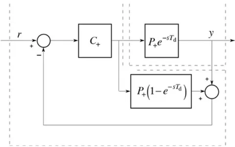
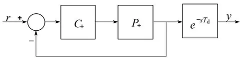
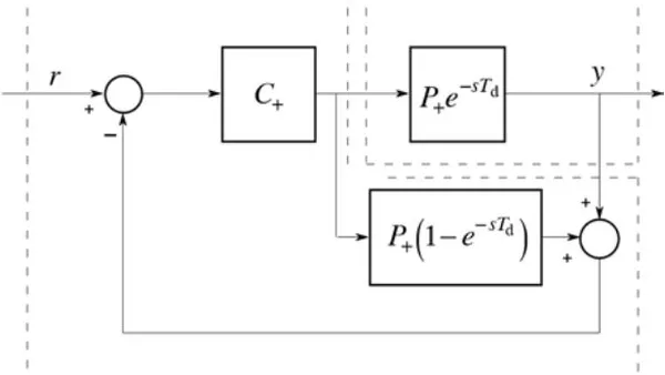
It is easy to check that the SMITH predictor is equivalent to the scheme shown in Fig. 2. This figure clearly shows that the regulator $C_{+}$ can be designed to the delay free $P_{+}$, independently of the time delay $T_{\mathrm{d}}$. This scheme explains why the SMITH predictor is also called SMITH regulator [8], [9], [10]. The whole procedure is, of course, not independent of $T_{\mathrm{d}}$, because the predictor scheme contains block depending on the delay.

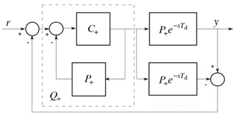
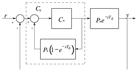
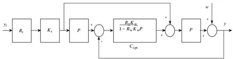
It is possible to redraw the SMITH predictor into further schemes, which allow special interpretations. Fig. 3. shows another equivalent scheme what corresponds to the well known Internal Model Control (IMC) scheme and principle. Fig. 4. presents the resulting closed-loop with the serial regulator $C_s$ equivalent to the application of the SMITH predictor.

II. THE YOULA PARAMETERIZATION

A YOULA-parameterized (YP) closed-loop [4], [8] is shown in Fig. 5, where e is the error, $u$ is the regulator output and w is the output disturbance signal, respectively.

Here the plant $P$ is stable and the $A/-\underset{―}{\text{RealizableStabilizing}}$ (ARS) regulator is

The closed-loop transfer function or Complementary Sensitivity Function (CSF)

which is linear in the stable YOULA parameter $Q$.

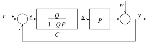
It is well known that the $YP$ regulator corresponds to the classical IMC structure shown in Fig.

6, where $r$ is the reference signal, $u$ is the regulator output, $y$ is the output signal and $w$ is the output disturbance signal, respectively. If there is no disturbance and the internal model is equal to the process transfer function, the signal fed back to the reference signal is zero, and the forward path $QP$ determines the reference signal tracking. The feedback loop rejects the effect of the disturbance and of the plant/model mismatch.

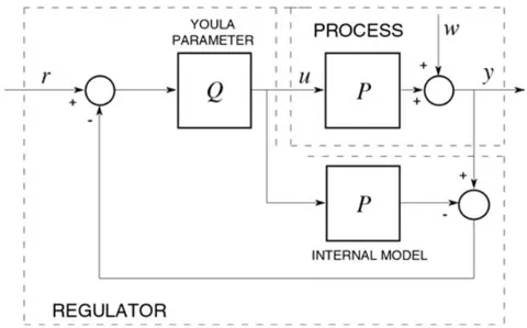
It can also be well seen that $Q_{+}$ in Fig. 3 corresponds to the YOULA parameter. For a more detailed comparison consider the extension of $YP$ regulator for more general case next.

III. A G2DOF CONTROLLER FOR STABLE LINEAR PLANTS

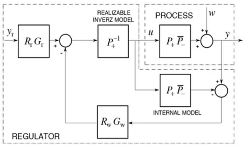
The first systematic method introducing the generic two degree of freedom (G2DOF) scheme was presented in [5], [8], [9], [10] when the process is open-loop stable and it is allowed to cancel the stable process poles, which case occurs at many practical tasks. 2DOF in this approach means that the dynamics of reference signal tracking and that of disturbance rejecting are different. This framework and topology is based on the $YP$ providing ARS regulators for open-loop stable plants and capable to handle the plant time-delay, too.

A G2DOF control system is shown in Fig. 7 for the stable process

which is more general than what was used in (1), because here $P_{+}$ is stable and Inverse-Stable-Realizable (ISR), $P_{-}$ is Inverse-Unstable-Unrealizable (IUU).

The optimal ARS regulator of the G2DOF scheme can be given by an explicit form

where $y_t$ is the tracking (servo) and $y_d$ is the regulating (or disturbance rejection) independent behaviors of the closed-loop response, respectively. So the delay $e^{-s{T}_d}$ and $P_{-}$ can not be eliminated, consequently the ideal design goals $R_r$ and $R_w$ are biased by $G_r{P}_{-}$ and $G_w{P}_{-}$. Here $R_r$ and $R_w$ are assumed stable and usually strictly proper transfer functions, that are partly capable to place desired poles in the tracking and the regulatory transfer functions, furthermore they where

is the associated optimal $Y$ -parameter. Furthermore

The YP regulator (5) can be considered the generalization of the TRUXAL-GUILLEMIN [2], [8], [9], [10] method for stable processes.

It is interesting to see how the transfer characteristics of the closed-loop look like:

are usually referred as reference signal and output disturbance predictors. They can even be called as reference models, so reasonably $R_{\mathrm{r}}(\omega =0)=1$ and $R_{\mathrm{w}}(\omega =0)=1$ are selected. The unity gain of $R_{\mathrm{w}}$ ensures integral action in the regulator, which is maintained if the applied optimization provides $G_{\mathrm{w}}{P}_{-}(\omega =0)=1$.

The role of $R_{\mathrm{r}}$ and $R_{\mathrm{w}}$ (predictors or filters) is threefold.

They prescribe the tracking and regulatory properties of the control loop. They influence the magnitude of the actuating signal and also influence the robustness properties of the control system.

An interesting result was found [6] that the optimization of the G2DOF scheme can be performed in ${\mathsf{H}}_2$ and ${\mathsf{H}}_{\mathrm{\infty }}$ norm spaces by the proper selection of the serial embedded filters $G_{\mathrm{r}}$ and $G_{\mathrm{w}}$ attenuating the influence of the invariant process factor $P_{-}$. Using

${\mathsf{H}}_2$ norm a Diophantine-equation (DE) should be solved to optimize these filters. If the optimality requires a ${\mathsf{H}}_{\mathrm{\infty }}$ norm, then the NEVANLINNA-PICK (NP) approximation is applied.

After some straightforward block manipulations the G2DOF control system can be transformed to another form shown in Fig. 8, which is the generalized version of the classical IMC scheme in Fig. 6.

IV. SMITH PREDICTOR AS A SUBCLASS OF G2DOF CONTROLLER

The previous two sections clearly show that the SMITH predictor is a special subclass of the G2DOF controllers with a $YP$ parameterized regulator

if $C_{+}$ is stabilizing $P_{+}$, i.e., the delay free part of the process. Here the special CSF

characterizing the closed-loop in Fig. 2 is the reference model $R_{+}$ and $L_{+}=C_{+}{P}_{+}$ is its loop transfer function.

It is also easy to see that the resulting serial regulator of the SMITH predictor in Fig. 4 is

This formula presents the possible way of realization for a continuous-time (CT) case. Here $K_{\mathrm{S}}$ denotes a serial factor modifying the original $C_{+}$ regulator of the SMITH predictor

At the stability limit cross over frequency ${\omega }_{\mathrm{c}}$ where $L_{+}=-1$ the factor $K_{\mathrm{s}}$ takes a considerable positive phase advance into the closed-loop

This is the simple physical explanation of the success of the SMITH predictor [3].

Some early evaluations state that unfortunately the SMITH predictor is only good for tracking and not for disturbance rejection. This evaluation is wrong. The SMITH regulator was proposed for a one-degree of freedom (1DOF) closed-loop, so it is naturally not for 2DOF purposes. The real problem of the SMITH regulator is that it allows the design of the closed-loop only via an indirect way by selecting $R_{+}=T_{+}$, while the design procedure of the G2DOF scheme gives a direct procedure to design the independent tracking and disturbance rejection properties. This means that the original idea of SMITH was that a classical design of $T_{+}$ is necessary for the proper application. One must know that the YOULA parameterization and its application for regulator design was unknown for Otto SMITH when he invented his predictor.

V. THE DISCRETE-TIME VERSION OF G2DOF CONTROLLER

Although (11) suggests a proper way how to realize the SMITH regulator, it is not realistic to build any regulator containing the $e^{-s{T}_{\mathrm{d}}}$ delay element for continuous-time case. In the practice only the discrete-time (DT) version can be applied by computer realization. Consider the DT model of the CT process in the form of its pulse transfer function given by

where $G_{+}$ is stable and $ISR$, $G_{-}$ is $IUU$ and $z^{-d}$ corresponds to the discrete time-delay, where $d$ is the integer multiple of the sampling time. (In a practical case the factor $G_{-}$ can incorporate the underdamped zeros and the neglected poles providing realizability, too). The optimal ARS regulator of the G2DOF scheme can be given now by

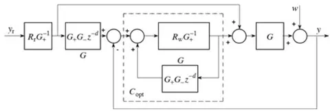
which corresponds to the CT case of (5), furthermore (6) and (7) are formally exactly the same for DT case. The transfer characteristics of the closed-loop is now

Because the optimization of the embedded filters $G_{\mathrm{r}}$ and $G_{\mathrm{w}}$ requires special knowledge and practice of getting the solution from a DE and NP approximation, suboptimal design is mostly applied assuming $G_{\mathrm{r}}=G_{\mathrm{w}}=1$. In such cases the influence of the invariant process factors are not attenuated at all, so they appear in the closed-loop characteristics (15) directly. Such G2DOF control scheme is shown in Fig.

It follows from the above discussion that it is not necessary to apply the classical SMITH predictor principle, instead it is more effective to use the regulator design procedure of the G2DOF controller scheme.

Fig. 9: Discrete-Time G2DOF Control System for the Suboptimal $G_{\mathrm{r}}=G_{\mathrm{w}}=1$ case

VI. SIMPLE EXAMPLES

Example 1

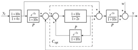
Consider a very simple first order time-delay process

The tracking and disturbance rejection reference models are

Here $P_{-}=1$, therefore $G_{\mathrm{r}}=G_{\mathrm{w}}=1$ is the optimal selection for the embedded filters.

Design a YOULA-parameterized optimal regulator.

and the optimal serial compensator is

Both transfer functions are realizable.

Because $C_{\mathrm{opt}}(s=0)=\mathrm{\infty }$ the regulator is integrating obtained from the condition $R_{\mathrm{w}}(s=0)=1$. The optimal

It is easy to check that the closed-loop characteristics is

according to the general theory.

Example 2

Consider the DT model of a very simple first order time delay process

It is required to speed up the process by a closed-loop.

Design a YP controller. Select the reference models

Because $G_{-}=1$, there is no optimization task, so the selections $G_{\mathrm{r}}=1$ and $G_{\mathrm{w}}=1$ are optimal. The optimal regulator is

and the serial compensator is

The optimal final closed-loop is shown in Fig. 11. Observe that $C_{\mathrm{opt}}(z=1)=\mathrm{\infty }$, i.e. the regulator is an integrating one, which follows from the condition $R_{\mathrm{w}}(z=1)=1$.

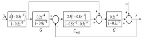
The closed-loop characteristics is

which exactly corresponds to our design goals.

This example shows that there is no applicability problem for DT regulator design. These filters are easy to be realized in a computer controlled system.

Example 3.

The continuous first order plant with significant time delay is given by the transfer function

The plant is sampled with sampling time $T_s=5$ sec and a zero order hold is applied at its input. Let us design a PI controller ensuring about ${60}^{\circ }$ of phase margin, a Smith predictor and a YOULA-parameterized controller. Compare the reference signal tracking and output disturbance rejection behaviour of the three control systems. Demonstrate the effect of time delay mismatch.

The pulse transfer function of the plant is

The pulse transfer function of the $PI$ controller [7] applying pole cancellation with a gain ensuring the required phase margin is

The SMITH predictor controller $C_{+}$ is designed for the delay free process as a PI controller and it is obtained as

Then it is transformed to the SMITH predictor form according to the discretized version of (11).

In the case of the YOULA parameterized controller let us choose the disturbance filter

and the reference filter as

whose pulse transfer functions are

Fig. 12: Step response and disturbance rejection dynamics of the $PI$, SMITH and YOULA controllers

The YOULA parameter supposing $G_{\mathrm{r}}=G_{\mathrm{w}}=1$ is

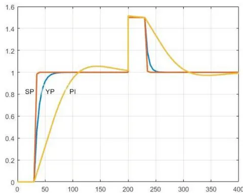
Figure 12 shows the step response and a shifted step disturbance rejection of the three controllers.

It is seen that in case of significant time delay SMITH predictor and the YOULA parameterized controllers ensure significant acceleration compared to the PI controller.

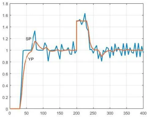
Figure 13 demonstrates the effect of time delay mismatch in the case of the SMITH and the YOULA controllers. The time delay of the model is 30, while the time delay of the process is 33.

It is seen that the YOULA parameterized controller tolerates much better the inaccuracy of the parameter than the SMITH predictor. While the SMITH predictor is very sensitive to the inaccuracies in the parameters (it is not robust), the filters in the YOULA parameterized controller can be designed for robust behaviour [11].

These are, of course, very simple examples standing only to present the simplicity of the G2DOF controller scheme, which should replace the classical approach of a SMITH predictor.

VII. CONCLUSIONS

The SMITH predictor is a classical method of handling time-delay in closed-loop control design. It is shown that this method is a subclass of the YP based G2DOF control scheme. An obvious drawback of the SMITH predictor is that the closed-loop properties cannot be designed directly using simple algebraic methods, which is possible in the G2DOF structure. The G2DOF scheme allows even the optimal attenuation of the invariant process factors. The appropriate choice and design of the filters allows to influence such important properties as performance and robustness. So the paper suggests to use the newer methodology to design DT controllers for time-delay processes.

The role of the SMITH predictor remains important in the history of control engineering, because it was one of the first, easy to use and widely applied method to simply eliminate the influence of the delay in the design of closed-loop control properties. Nevertheless this method is sensitive to the accurate knowledge of the time delay.

The recent theoretical developments and easily applicable algebraic design methods allow to use more effective and more general controller design procedures.