## I. INTRODUCTION
CPU scheduling is a fundamental practice in the realm of operating systems, orchestrating the execution of processes to efficiently utilize the CPU. This practice becomes necessary when a process must seize CPU control while another process is temporarily halted in a waiting state, typically due to resource unavailability, such as I/O operations. The primary objectives of CPU scheduling are to enhance system effectiveness, responsiveness, and fairness while maximizing CPU utilization.
Process scheduling, an integral component of multiprogramming operating systems, involves managing the transition of processes in and out of the CPU based on a specific strategy. These operating systems can load multiple processes into executable memory concurrently, allowing them to share the CPU through time multiplexing.
There are two principal categories of CPU scheduling algorithms: preemptive and non-preemptive. In preemptive scheduling, a process allocated to the CPU can be interrupted, and its running state may be changed to a waiting state. This approach is known for temporarily suspending logically runnable processes and is referred to as preemptive scheduling. However, frequent arrivals of high-priority processes in the ready queue can potentially lead to starvation for lower-priority processes. It's important to note that preemptive scheduling comes with the overhead of managing these process interruptions.
In contrast, non-preemptive scheduling ensures that once a process gains access to the CPU, it retains control until its execution is complete. The CPU cannot be forcibly taken away from the process until it finishes its execution. In this scenario, a process voluntarily releases the processor only after its task is done.
While various CPU scheduling algorithms exist, some common ones include First In First Out (FIFO), Shortest Job First (SJF), Priority Scheduling, and Round Robin CPU Scheduling. Each of these algorithms offers unique advantages and trade-offs in managing the CPU's allocation to processes.
## II. LITERATURE SURVEY
In FCFS scheduling, jobs are executed in the order they arrive, following a "first come, first served" principle [1]. This algorithm can operate in both non-preemptive and preemptive modes depending on system requirements. It is easy to understand and implement, relying on a First-In-First-Out (FIFO) queue. However, FCFS suffers from the drawback of high average waiting times, limiting its overall performance.
Shortest Job First (SJF), also known as Shortest Job Next, prioritizes tasks based on their execution time [3]. It can function as both a preemptive and non-preemptive algorithm. SJF is particularly effective in reducing waiting times, making it a preferred choice in batch systems where CPU time requirements are known in advance. However, it is impractical for interactive systems where predicting CPU time is challenging.
Priority scheduling is a non-preemptive algorithm commonly used in batch systems [5]. Each process is assigned a priority, with the highest-priority process scheduled first, followed by processes of equal priority in a first-come-first-served manner. Priorities can be assigned based on memory, time, or other resource requirements.
Round Robin is a preemptive scheduling algorithm where each process is allocated a fixed time quantum for execution [8]. When a process's time quantum expires, it is preempted, and another process is allowed to execute for its allocated time period. Context switching is necessary to manage preempted processes effectively.
Multiple-level queues are a manual scheduling algorithm [15] that leverages various existing algorithms to categorize jobs based on common characteristics. Multiple queues are maintained for processes with similar attributes, each with its specific scheduling algorithm [8]. Priorities are assigned to each queue, enabling effective organization. For instance, OS-bound jobs can be grouped in one queue, while I/O-bound jobs reside in another. The Process Scheduler selects jobs from each queue based on the algorithm associated with that queue. Multi-level queue scheduling was developed for scenarios where processes naturally belong to different groups.
## III. SHORTCOMINGS OF EXISTING ALGORITHM
We have evaluated the conventional Round Robin (RR) algorithm as our baseline scheduling approach. The RR algorithm is generally considered efficient because it ensures that all processes in the process set have an equal opportunity for execution. However, our research has identified that our system comprises both critical processes with high priority and normal (low-priority) processes. A significant limitation of the RR algorithm is its lack of consideration for process priorities, which we regard as a major drawback.
To address this limitation, we have proposed a novel methodology aimed at enhancing the RR algorithm's effectiveness.
Let's now consider the following set of processes with a fixed time quantum of 4.
Table 1: For the Existing Methodology, Processes in the Ready Queue
<table><tr><td>Process Name</td><td>Priority</td><td>Burst Time</td></tr><tr><td>P0</td><td>0</td><td>5</td></tr><tr><td>P1</td><td>1</td><td>3</td></tr><tr><td>P2</td><td>1</td><td>12</td></tr><tr><td>P3</td><td>0</td><td>9</td></tr><tr><td>P4</td><td>0</td><td>8</td></tr></table>
Round Robin scheduling is known for its ability to ensure a fair chance for every process in the set to execute. Consequently, Figure 1 illustrates the Gantt chart and waiting times for the given set of processes.
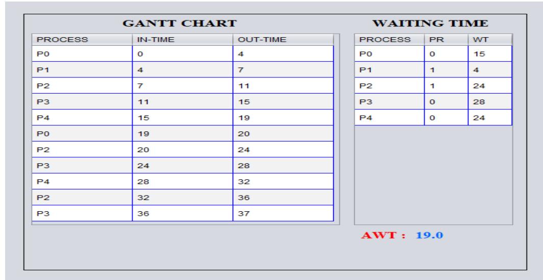 Figure 1: Gantt chart of Existing Methodology
The average waiting time (AWT) for processes with both low and high priorities is presented in Figure 2 below.
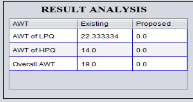 Figure 2: Waiting Time Analysis of Existing Methodology
## IV. PROPOSED METHOD
The Round Robin algorithm operates under the premise of treating all jobs with equal priority, executing processes one at a time for a specific duration known as the Time Quantum (TQ). A process can continue running until either its time quantum (TQ) is exhausted or it completes its CPU burst time. Within the system, processes have varying priorities, distinguishing between high-priority critical tasks, which demand immediate CPU attention, such as shutting down the computer due to overheating or issuing alerts for unauthorized access, and normal-priority processes, which encompass all other standard tasks.
## V. PROPOSED ALGORITHM
Our proposed algorithm is given below.
Step 1: Input process details, including the process name, priority, and burst time.
Step 2: Save the collected information in a queue labeled as "READYQ."
Step 3: Establish two distinct queues: "HIGHPQ" for high-priority processes and "LOWPQ" for regular-priority processes.
Step 4: Repeat steps 5 to 11 until the remaining CPU burst times for processes in both "HIGHPQ" and "LOWPQ" reach zero.
Step 5: Choose the next process from "HIGHPQ" or "LOWPQ" alternatively, with the initial selection favoring "HIGHPQ" to give higher-priority tasks precedence.
Step 6: If the selected process has a remaining CPU burst time greater than or equal to the time quantum, proceed to step 7; otherwise, go to step 8.
Step 7: Execute the chosen process for the duration of the time quantum.
Step 8: Continue executing the selected process until its remaining burst time reaches zero.
Step 10: Record the process's IN-TIME and OUT-TIME in a table known as the GANTTCHART.
Step 11: If the previous process was selected from "HIGHPQ," switch the next turn to "LOWPQ," and vice versa.
In this study, I have introduced an approach that ensures high-priority processes receive precedence in execution. The methodology I've suggested involves granting alternating opportunities to both high and low priority processes. It begins by selecting a process from the high-priority queue, followed by the selection of the next process from the low-priority queue. The following steps outline the proposed methodology.
HIGHPQ- This queue contains the processes of high priority.
<table><tr><td>Process Name</td><td>Priority</td><td>Burst Time</td></tr><tr><td>P1</td><td>1</td><td>3</td></tr><tr><td>P2</td><td>1</td><td>12</td></tr></table>
LOWPQ- This queue contains the processes of low priority.
<table><tr><td>Process Name</td><td>Priority</td><td>Burst Time</td></tr><tr><td>P0</td><td>0</td><td>5</td></tr><tr><td>P3</td><td>0</td><td>9</td></tr><tr><td>P4</td><td>0</td><td>8</td></tr></table>
Below, in Figure 3, you can observe the Gantt chart and waiting times for the processes listed in Table 1, using a time quantum of 4.
GANTT CHART
<table><tr><td>PROCESS</td><td>IN-TIME</td><td>OUT-TIME</td></tr><tr><td>P1</td><td>0</td><td>3</td></tr><tr><td>P0</td><td>3</td><td>7</td></tr><tr><td>P2</td><td>7</td><td>11</td></tr><tr><td>P3</td><td>11</td><td>15</td></tr><tr><td>P2</td><td>15</td><td>19</td></tr><tr><td>P4</td><td>19</td><td>23</td></tr><tr><td>P2</td><td>23</td><td>27</td></tr><tr><td>P0</td><td>27</td><td>28</td></tr><tr><td>P3</td><td>28</td><td>32</td></tr><tr><td>P4</td><td>32</td><td>36</td></tr><tr><td>P3</td><td>36</td><td>37</td></tr></table>
WAITING TIME
<table><tr><td>PROCESS</td><td>PR</td><td>WT</td></tr><tr><td>P0</td><td>0</td><td>23</td></tr><tr><td>P1</td><td>1</td><td>0</td></tr><tr><td>P2</td><td>1</td><td>15</td></tr><tr><td>P3</td><td>0</td><td>28</td></tr><tr><td>P4</td><td>0</td><td>28</td></tr></table>
AWT:18.8
Figure 3: Working of Proposed Methodology
## VI. RESULT AND ANALYSIS
The figure below illustrates the application of the proposed algorithm, resulting in an average waiting time for high-priority processes of approximately 7.5. This value is nearly half of the average waiting time observed when using the existing algorithm. Furthermore, the overall waiting time for the process set is significantly reduced through the implementation of the proposed algorithm.
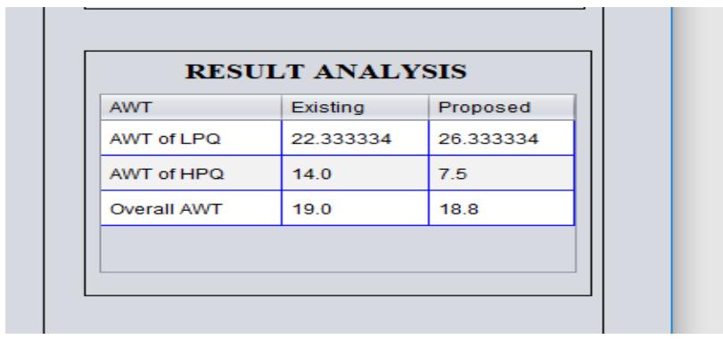 Figure 4: Result Analyses of Existing Vs Proposed Methodology
The same result can be analyzed using bar chart shown in figure 5.
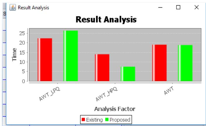 Figure 5: Result Analysis of Existing Vs Proposed Methodology Using Bar chart
## VII. CONCLUSION
In this study, I've maintained the core principle of traditional round-robin scheduling, which aims to ensure that all processes receive an equal opportunity to execute within a specific time quantum. The innovation lies in the strategic placement of high-priority processes at the rear of the ready queue, preventing them from being excessively delayed by late arrivals. The proposed approach is expected to reduce the average waiting time for high-priority processes, but it may lead to an increase in the average waiting time for normal priority processes. The overall average waiting time for all processes within the ready queue may exhibit improvement or remain unchanged, contingent on the specific mix of processes.
Although the proposed algorithm demonstrates enhanced performance for high-priority processes, there remains an ongoing drive for continued improvement. In the future, these results could potentially be refined by introducing variable time quantum strategies. Furthermore, optimizing the algorithm's execution can be accomplished by leveraging more efficient data structures.
Generating HTML Viewer...
References
26 Cites in Article
Sanjay Kumar,Panda,Saurav Kumar,Bhoi (2012). An Effective Round Robin Algorithm using Min-Max Dispersion Measure.
Abraham Silberschatz,Peter Baer Galvin,Greg Gagne Operating System Concepts.
H Rakesh Mohanty,Khusbu Behera,Monisha Patwari,Dash (2010). Design and Performance Evaluation of a New Proposed Shortest Remaining Burst Round Robin (SRBRR) Scheduling Algorithm.
Abdulrazaq Abdulrahim,Saleh E. Abdullahi,Junaidu B. Sahalu (2014). A New Improved Round Robin (NIRR) CPU Scheduling Algorithm.
Pallab Banerjee,Probal Banerjee,Shweta Sonali Dhal (2012). Comparative Performance Analysis of Average Max Round Robin Scheduling Algorithm (AMRR) using Dynamic Time Quantum with Round Robin Scheduling Algorithm usingStatic Time Quanmtum.
P Varma (2013). A Finest Time Quantum for Improving Shortest Remaining Burst Round Robin (SRBRR) Algorithm.
Srishty Jindal,Grover (2014). Round Robin CPU Scheduling Using Dynamic Time Quantum with Multiple Queue.
Rakesh K.Lenka,Prabhat Ranjan (2012). A 2LFQ Scheduling with Dynamic Time Quantum using Mean Average.
(2014). A MODIFIED ROUND ROBIN CPU SCHEDULING ALGORITHM WITH DYNAMIC TIME QUANTUM..
A Silberschatz,P Galvin,G Gagne Operating Systems Concepts.
Sanjaya Kumarpanda,Debasis Dash,Jitendra Kumar Rout (2012). A Group based Time Quantum Round Robin Algorithm using Min-Max Spread Measure.
(2014). Designing Various CPU Scheduling Techniques using SCILAB.
(2009). Self-Adjustment Time Quantum in Round Robin Algorithm Depending on Burst Time of the Now Running Processes.
R Matarneh (2009). Seif-Adjustment Time Quantum in Round Robin Algorithm Depending on Burst Time of the Now Running Proceses.
H Behera,R Mohanty,D Nayak (2010). A New Proposed Dynamic Quantum with Re-Adjusted Round Robin Scheduling Algorithm and Its Performance Analysis.
Ajit Singh,Priyanka Goyal,Sahil Batra (2010). An Optimized Round Robin Scheduling Algorithm for CPU Scheduling.
J Rami,Matarneh (2009). Self-Adjustment Time Quantum in Round Robin Algorithm Depending on Burst Time of Now Running Processes.
Abdulrazaq Abdulrahim,Saleh E. Abdullahi,Junaidu B. Sahalu (2014). A New Improved Round Robin (NIRR) CPU Scheduling Algorithm.
Sourav Kumar Bhoi,Sanjaya Kumar Panda,Debashee Tarai (2011). Enhancing cpu performance using subcontrary mean dynamic round robin (smdrr) scheduling algorithm.
H Rakesh Mohanty,Khusbu Behera,Monisha Patwari,Dash (2010). Design and Performance Evaluation of a New Proposed Shortest Remaining Burst Round Robin (SRBRR) Scheduling Algorithm.
Ishwari Singh,Rajput (2012). A Priority based Round Robin CPU Scheduling Algorithm for Real Time Systems.
Manish Kumar,Mishra,Abdul Khan (2012). An Improved Round Robin CPU Scheduling Algorithm.
P Varma (2013). A FINEST TIME QUANTUM FOR IMPROVING SHORTEST REMAINING BURST ROUND ROBIN (SRBRR) ALGORITHM.
Rakesh Kumar Yadav,K Abhishek,Navin Mishra,Himanshu Prakash,Sharma (2010). An Improved Round Robin Scheduling Algorithm for CPU Scheduling.
No ethics committee approval was required for this article type.
Data Availability
Not applicable for this article.
How to Cite This Article
Debashish Barman. 2026. \u201cOptimized Round Robin CPU Scheduling for Critical Processes\u201d. Global Journal of Computer Science and Technology - H: Information & Technology GJCST-H Volume 23 (GJCST Volume 23 Issue H3).
Explore published articles in an immersive Augmented Reality environment. Our platform converts research papers into interactive 3D books, allowing readers to view and interact with content using AR and VR compatible devices.
Your published article is automatically converted into a realistic 3D book. Flip through pages and read research papers in a more engaging and interactive format.
Our website is actively being updated, and changes may occur frequently. Please clear your browser cache if needed. For feedback or error reporting, please email [email protected]
Thank you for connecting with us. We will respond to you shortly.