## I. INTRODUCTION Intelligent Transportation Systems (ITs) are one of the most anticipated smart city services and have already seen widespread adoption. The Sydney Coordinated Adaptive Traffic System (SCATS) is a fully adaptive urban traffic control system that optimizes traffic flow and currently operates in more than 37,000 intersections worldwide. Optimizing traffic flow conditions not only shortens travel times but can also reduce the carbon emissions generated from road vehicle activity [5]. Unfortunately, city-wide traffic control models are difficult to study using realworld data. While it is possible to develop a model of an ITS using historical data, it is difficult to determine its effectiveness because traffic conditions would morph under the use of the ITS. Therefore, instead of considering city-wide coordination, this research focuses on intelligent routing based on real-time prevailing traffic conditions, similar to the service provided by Google Maps. Traditional traffic flow models rely on shallow learning algorithms and only a few conditions to predict traffic flow. While these models have been moderately successful, they fail to capture the deeper relationship between their features and also fail to adapt to changing conditions quickly [17]. Deep learning methods, on the other hand, have drastically improved the state-of-the-art in a variety of fields, such as speech recognition and object detection. Deep learning's success is largely based on its ability to discover intricate structures and relationships between features in large datasets [9]. The evolution of traffic flow over time is dynamic and nonlinear, which makes it a perfect candidate for deep learning methods. With the advent of the Internet of Things (IoT), wireless sensors are able to capture a variety of real-world conditions such as traffic accidents, weather, and external events like sports games. ITSs are then able to aggregate these features to build hybrid multimodal methods for traffic flow forecasting using deep learning [7,10]. However, this data transmission and analysis must be performed at ultra-low latency and in real time in order to have the intended effect of optimizing the operations of a smart city. The combination of compute-intensive workloads and latency-sensitive applications motivates the use of real-time cloud computing. [8] have recently introduced a framework for efficient edge and cloud computing specifically designed for ITSs but do not provide empirical results to substantiate their claims. Moreover, current clouds lack service level agreements on latency; these clouds provision resources and not latency. Such a service level agreement is critical for applications like ITSs. In this paper, I empirically study the latency performance of a simplified ITS on a real-time cloud. The rest of this paper is organized as follows. Section II presents related work. In Section III, I provide relevant background information for the technologies used. Section IV covers design and implementation strategies. Section V presents my empirical study using a real traffic dataset and evaluates the latency of the application on a real-time cloud. Finally, Section VI offers conclusions and directions for future research. ## II. RELATED WORK Traffic flow forecasting has a long history in transportation literature, and many techniques have been proposed to address this problem. [17] introduce an autoregressive integrated moving average (ARIMA) process for estimating traffic flows. While the ARIMA model has the benefit that it is easy to interpret, it is not able to accurately capture the non-linear, stochastic nature of traffic flow evolution. [13] have utilized an efficient Bayesian particle filter for tracking traffic flows and demonstrated its effectiveness on a dataset from the I-55 highway system in Illinois. The authors then used the same dataset to evaluate a deep neural network with $\ell_1$ regularization and applied this model to predict traffic flows during a baseball game accurately [14]. [11] develop a novel model, called LC-RNN, that combines both convolutional and recurrent neural networks in order to learn the time-series and spatiotemporal nature of traffic patterns more meaningfully. While deep-learning, specifically time-series-based approaches, have seen the greatest empirical success, it is apparent that no single method works best for every situation. In general, the most successful methods are hybrid methods that can combine techniques to improve the accuracy of prediction under the prevailing traffic conditions [4]. ### a) Traffic Flow Traffic flow forecasting is a challenging problem in the space of intelligent traffic management. In this paper, I consider traffic flow in a macroscopic context. That is, instead of considering each vehicle in a traffic stream individually, I rather think of the traffic flow as a measurement at a single fixed location in space. The traffic flow forecasting problem is thus formally defined as follows. At time $T$, I seek to predict the future traffic flow $q_{T+1}$ at time $T + 1$ or $q_{T+n}$ at time $T + n$ based on the history of traffic data. Flow may be considered a temporal measurement and is usually expressed in terms of units over a period of time. For a single lane of traffic, I can define the flow $q$ in region $R$ as $$ q = \frac {N}{T}, \tag {1} $$ where $N$ is the number of vehicles observed crossing region $R$ during timespan $T$ [12]. For multiple-lane traffic, I can sum the partial flows across each of the $L$ lanes $$ q = \sum_{l=1}^{L} q_{l} = \frac{1}{T} \sum_{l=1}^{L} N_{l}, $$ where $N_{l}$ is the number of vehicles that passed a detector's site in lane $l$. I also define the mean speed of the traffic stream, expressed in terms of miles (or kilometers) per hour. In this paper, I consider the time-mean speed, which is calculated as the arithmetic average of the vehicles' instantaneous speeds in the region $R_{t}$. The time-mean speed is denoted by $v_{t}^{-}$ $$ \bar {v} _ {t} = \frac {1}{N} \sum_ {i = 1} ^ {N} v _ {i}, \tag {3} $$ where $v_{i}$ is the instantaneous speed of the $i$ th vehicle [12]. ### b) Vanishing Gradient The vanishing gradient problem as described in [3] is particularly prevalent in training recursive neural networks. Most neural networks learn weight parameters through some gradient-based optimization method, such as backpropagation through time. For deep or recursive neural networks, backpropagation yields lengthy update equations in which gradients may become vanishingly small, effectively preventing the weight from ever updating its value. There are many methods to combat the vanishing gradient problem in recurrent neural networks, namely the introduction of long short-term memory networks. ### c) Long Short-Term Memory Networks Given their capacity to memorize long-term dependencies, long short-term memory (LSTM) neural networks have special advantages for traffic flow prediction. LSTMs are a specific type of recurrent neural network. Recurrent neural networks are comprised of memory cells; memory cells add a loop to the traditional perceptron model of a neural network. These loops make the network recursive, thereby allowing information to persist. Recurrent neural networks have been notable in language modeling, speech-to-text transcript, and other applications with time-series patterns. Whereas traditional recurrent neural networks suffer from the vanishing gradient problem during training, LSTM networks are specifically designed to address the vanishing gradient problem [15]. Just like recurrent neural networks, LSTMs are comprised of many memory cells. LSTM networks combat the vanishing gradient problem through the use of forgetting gates, which are special structures added to the memory cell designed to allow the cell to forget certain information. The typical structure of an LSTM memory cell is shown in Figure 1. 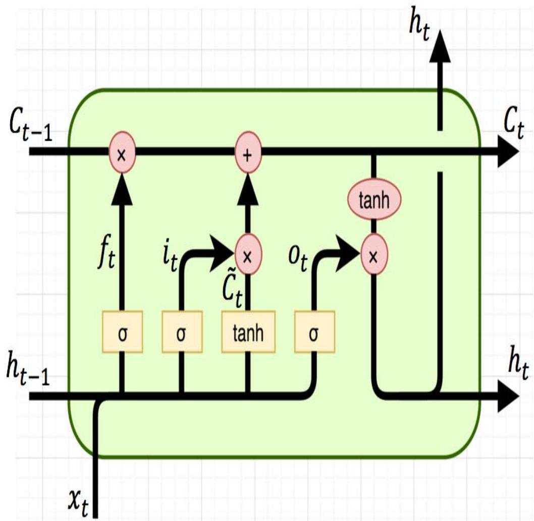 Fig.1: Structure of LSTM Memory Cell [15] describes the information flow for a typical LSTM memory cell—an LSTM memory cell has three gates: an input gate, a forget gate, and an output gate. Each of these gates is a way to let information flow optionally and is comprised of a sigmoid activation function. The sigmoid function squashes values between the range of [0, 1], representing how much information to let through a given gate. At the $t$ th timestep, the output from the previous LSTM memory cell, $h_{t-1}$, is fed into the forget gate, which determines how much information from the previous gate to keep, $f_t$. The output of the forget gate is then multiplied by the previous cell state. The input gate determines how much information from the most recent observation, $x_t$, to include in the cell state. The current cell state, $C_t$ is first passed through the tanh activation function and then multiplied with the output from the input gate, $i_t$, yielding $C_t$. Finally, the current cell state, $C_t$ is updated: $$ C _ {t} = f _ {t} * C _ {t - 1} + i _ {t} * \tilde {C} _ {t} \tag {4} $$ The updated cell state, $C_t$, is then fed into the output gate, which determines the output from the current cell state using the sigmoid function, producing $o_{t}$. The memory cell applies the tanh activation function to the current cell state to squash the values between $[-1,1]$ and multiplies the result with $o_{t}$, producing: $$ h _ {t} = o _ {t} * \tanh \left(C _ {t}\right) \tag {5} $$ While training LSTM networks takes a very long time, stacking many of these LSTM memory cells produces an extremely powerful model capable of learning long-term dependencies, which is particularly useful for predicting traffic flow [10]. ### d) A Star Search The A Star Search Algorithm $(A^{*})$ is an algorithm used in graph traversal to find the optimal path between any pair of nodes. In my case, I can express a city's roads and freeways as a directed graph in which intersections are nodes, and the roads are edges. I can use $A^{*}$ to find the optimal path between any two points in the city. $A^{*}$ is an informed search algorithm that makes use of heuristics to decide which path to consider next. $A^{*}$ determines which path to consider next by minimizing the cost of the current path to the next node and the estimated cost from the next node to the end. Mathematically, this is expressed as- $$ f (n) = g (n) + h (n), \tag {6} $$ where $g(n)$ is the cost from the start node to node $n$, and $h(n)$ is a heuristic that estimates the cost from node $n$ to the end. In order for $A^*$ to be optimal, this heuristic must satisfy two properties: admissibility and consistency. An admissible heuristic is any such heuristic that does not overestimate the true cost of traveling to the next node. A consistent heuristic is any such heuristic that supports the following inequality for any two adjacent nodes, $x$ and $y$ $$ h (x) \leq \operatorname{dist} _ {x, y} + h (y) \tag{7} $$ ## III. BACKGROUND This section provides background on the Xen hypervisor and the scheduling framework in Xen. It also describes a stream-processing engine, Flink, and real-time messaging middleware, Kafka. ### a) Xen Xen [2] is a popular open-source virtualization platform that allows multiple virtual machines to share conventional hardware in a safe and resource-managed fashion. Xen serves as a virtual machine monitor (VMM) that lies between the hardware and guest operating systems. Xen controls a special domain called domain 0, which is responsible for managing all other guest domains. Each guest domain acts as a virtual machine (VM) and can specify its resource requirement in terms of the number of virtual CPUs (VCPUs). The typical Xen architecture is shown in Figure 2. Each VM has a guest operating system, which is responsible for scheduling tasks on to VCPUs. Xen is not only responsible for providing virtual resource interfaces to the VMs but is also responsible for scheduling the VMs onto physical CPUs (PCPUs). There are currently three different schedulers in Xen: Credit, Credit2, and RTDS. Credit is the default scheduler; it is a general-purpose weighted fair share scheduler. Credit2 is the evolution of the default credit scheduler; it is still based on a general purpose, a weighted fair share scheme, but it is more scalable and efficient with latency-sensitive workloads. RTDS is the real-time deferrable server scheduler that is specifically designed to handle real-time and latency-sensitive workloads [18]. 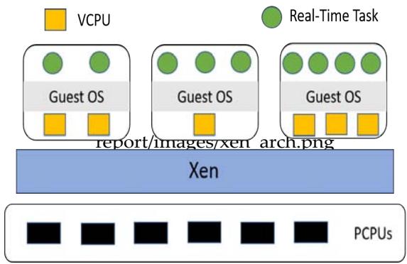 Fig. 2: Architecture of a Xen System Credit Under the Credit scheduler, each VM specifies a weight and optional cap. The weight corresponds to the share of CPU a VM will have relative to other VMs, and the cap encodes the maximum CPU resource a VM can receive. The scheduling algorithm itself is implemented with a partitioned queue: each PCPU maintains a local run queue of VCPUs, sorted by VCPU priority. While a VCPU is scheduled onto a PCPU, it burns credits; once the VM is preempted, VCPU priorities are recalculated based on the weight, cap, and amount of credits consumed. By default, CredituCreditwork stealing load-balancing scheme: if a PCPU has no VCPUs in its run queue, it will steal VCPUs from other cores. Credit2 The Credit2 scheduler is similar to the default Credit scheduler in that it focuses on fairness, but Credit2 also aims to address issues of latency and scalability. Credit2 uses a similar weighting scheme as Credit Credit, assigning a weight to each VM. Credit2, however, does not have support for caps like Credit credit and is also not CPU mask-aware. As a result, a VM cannot pin its workload to specific CPUs. RTDS Under the RTDS scheduler, each VM specifies a budget and period. While a VCPU is scheduled onto a PCPU, it consumes its budget until the budget is exhausted. The end of the period marks the deadline for a VCPU; at this time, any remaining budget is discarded, and then the budget is replenished. The scheduling algorithm is implemented using a global run queue sorted by VCPU deadline. This event-driven approach differs from the quantum-based approach used by the Credit and Credit2 schedulers. As a result, this avoids invoking the scheduler unnecessarily, which should reduce overhead. ### b) Apache Flink Apache Flink is a distributed stream-processing engine that provides data distribution, communication, and fault tolerance for distributed computations over data streams. Flink's programming model is a generalization of the MapReduce paradigm. The Flink API offers a set of useful transformation operations, such as join and filter, in addition to the traditional map and reduce functions. Applications specify a series of lazy transformations to an unbounded data stream, which are connected to sources and sinks. The Flink engine then uses a cost optimizer to determine an efficient execution plan called a dataflow. This dataflow is internally represented as a directed acyclic graph from sources to sinks with transformation operators in between. Sinks trigger the execution of the necessary lazy transformations [1]. ### c) Apache Kafka Apache Kafka is a distributed streaming platform that provides data pipelines and fault tolerance for streams of records across topics. Kafka makes use of two core APIs: the producer API allows an application to publish a stream of records to one or more topics, and the consumer API allows an application to subscribe to one or more topics and process the stream of records produced to them. Multiple producers may send streams of records on the same topic, and numerous consumers can also subscribe to the same topic. Each topic is spread over a cluster of Kafka brokers, with each broker holding at least one partition of the topic. Kafka uses Apache Zookeeper to help coordinate these services. Kafka is designed to meet high throughput and low latency requirements, making it an extremely suitable choice for real-time streaming applications. ## IV. DESIGN AND IMPLEMENTATION The previous section provided an overview of background information relevant to this paper's methodology. This section explores specific design and implementation choices. ### a) Dataset In order to create a model of an ITS, I needed historical traffic data to train and test a predictive model as well as data to use to study the latency of the application empirically. The California Transportation Performance Measurement System (PMS) collects real-time data from nearly 40,000 individual detectors across the freeway system in the state of California. PeMS provides data at a granularity of 5-minute intervals and includes features such as flow and average speed. These features are available across each lane and as aggregates for a given detector station. The raw data that comes from the single lanes is recorded every 30 seconds and then aggregated after every 5 minutes. While the real-time 30second granularity data is not made publicly available, the 5-minute granularity data is. For this research, I have downloaded data for March 2018 at 5-minute granularity. The data includes the timestamp, flow, and average speed (across individual lanes as well as aggregates); the data were taken from six different detector locations in southern California. Table 1 describes the detector locations and provides their latitude and longitude. Table 1: Detector Locations <table><tr><td>Detector Number</td><td>Canonical Name</td><td>Primary Freeway</td><td>Intersection</td><td>Latitude</td><td>Longitude</td></tr><tr><td>1</td><td>El Segundo</td><td>405S</td><td>105E</td><td>33.928621</td><td>-118.368522</td></tr><tr><td>2</td><td>Wilmington</td><td>405S</td><td>Wilmington</td><td>33.825757</td><td>-118.24005</td></tr><tr><td>3</td><td>Long Beach</td><td>405S</td><td>710S</td><td>33.824173</td><td>-118.207084</td></tr><tr><td>4</td><td>Athens</td><td>105E</td><td>110N</td><td>33.928478</td><td>-118.284031</td></tr><tr><td>5</td><td>Lynwood Gardens</td><td>105E</td><td>710S</td><td>33.914156</td><td>-118.184451</td></tr><tr><td>6</td><td>East Rancho Dominguez</td><td>710S</td><td>East Rancho Dominguez</td><td>33.877433</td><td>-118.192776</td></tr></table> ### b) Model of ITS I seek to create a model of an ITS that will predict future traffic flows and use this prediction to provide optimal routing using the $A^*$ algorithm. First, I must create a model that can forecast future traffic flows based on historical data. Evaluation Metric Given that this is a regression problem, I choose to train my models to minimize the mean squared error loss (MSE). MSE is defined as $$ L = \frac {1}{N} \sum_ {i = 1} ^ {N} \left(h _ {i} - y _ {i}\right) ^ {2}, \tag {8} $$ where $h_i$ is the predicted flow for the $i$ th test data point and $y_i$ is the true flow. Recall that the MSE loss metric is very sensitive to outliers and noise. To reduce this sensitivity, I preprocess my data by scaling non-time features between the range of 0 and 1. Once the network has been trained and I use it to predict traffic flows, I will transform the prediction back to its original scale. Algorithms 1 and 2 describe how I scale the data down before feeding input into the network and then transform the data back to its original scale to evaluate the network's performance. <table><tr><td>Algorithm 1: Preprocess Data</td></tr><tr><td>min←X.min;</td></tr><tr><td>max←X.max;</td></tr><tr><td>Xscaled←(X−min)/(max−min);</td></tr><tr><td>return Xscaled;</td></tr><tr><td>Algorithm 2: Transform Data to Original Scale</td></tr><tr><td>Xoriginal←Xscaled*(max−min)+min;</td></tr><tr><td>return Xoriginal;</td></tr></table> Comparison of Methods I chose to evaluate five different regression methods and select the model that gave the lowest MSE. I aggregate data across all six detector locations into one cumulative dataset and use this dataset to create a predictor. This cumulative dataset is used to develop a predicted model and empirically study the latency of my application on a real-time cloud. I split this dataset into training and testing sets; I used $80\%$ of the data for training and $20\%$ of the data for testing. Once the models had been trained, I measured their performance on the unseen test data again using MSE as a metric. Table 2 presents the MSE (on the original scale) as well as the mean absolute percentage error and $R^2$ value for each regressor. Although all models appear to perform extremely well on the dataset, I chose the LSTM neural network for two reasons. First, it is the model that has the lowest score. Second, as I have mentioned in Section II, LSTM neural networks are the state-of-the-art prediction method for forecasting traffic flows. In order to create the most realistic workload, I should select the model that is most likely to be used in a real-world context. Table 2: Model Scores <table><tr><td>Model</td><td>MSE</td><td>MAPE</td><td>R2</td></tr><tr><td>LSTM Neural Network</td><td>985.455275</td><td>23.091062</td><td>0.962043</td></tr><tr><td>Linear Regression</td><td>1013.644990</td><td>23.702992</td><td>0.960957</td></tr><tr><td>Random Forest</td><td>1083.919621</td><td>24.140704</td><td>0.958250</td></tr><tr><td>Gradient Boosting Decision Tree</td><td>1151.047555</td><td>25.586357</td><td>0.955664</td></tr><tr><td>Decision Tree</td><td>1988.652076</td><td>32.951715</td><td>0.923402</td></tr></table> LSTM I have implemented the LSTM neural network in Python using TensorFlow. Existing studies, such as [9], have shown that stacked LSTM layers in a neural network can lead to higher levels of representation of time-series data, which increases the effectiveness of the model. I adopted this architectural choice when I was working on the architecture. In order to prevent overfitting, I utilize dropout- a technique that randomly drops units and their connections during training [16]. The stacked LSTM layers are then connected to two fully connected layers. Recall that I preprocess the data and scale it to a range of 0 and 1, which is why the last layer only has one unit. I use the default activation function for the stacked LSTM layers, tanh, but select the rectified linear unit (ReLU) function in fully connected layers. ReLU is defined as $$ R e L U (x) = \max (0, x) \tag {9} $$ ReLU provides two primary benefits. First, it is very easy to compute relative to other activation functions like the sigmoid function or tanh, which speeds up training time. Furthermore, ReLU helps prevent the vanishing gradient problem during training. Table 3 summarizes neural network architecture. The network receives a 12x1 vector of scaled traffic flows as input, corresponding to the previous 12 observations of traffic flows, scaled between a range of 0 and 1, at 5-minute intervals. This vector represents the past hour's worth of traffic data. The network predicts the next value of flow, corresponding to traffic flow five minutes in the future. I can see from Table 2 that the trained LSTM neural network performs extremely well on test data. Since the network has been trained, I have used it as a predictor in my experiments. Table 3: LSTM Neural Network Architecture <table><tr><td>Layer Shape</td><td>Dropout</td><td>Activation</td></tr><tr><td>LSTM 256</td><td>N/A</td><td>tanh</td></tr><tr><td>LSTM 128</td><td>0.2</td><td>tanh</td></tr><tr><td>Dense 64</td><td>0.4</td><td>ReLU</td></tr><tr><td>Dense 1</td><td>N/A</td><td>ReLU</td></tr></table> Heuristic Recall that I use traffic prediction as a means of creating a heuristic for search algorithms. In order for the $A^{*}$ search algorithm to be optimal, the choice of heuristic must be admissible and consistent. I make use of the average speed measurement as well as the predicted flow in order to create a heuristic function. Consider the case in which I only use predicted flow in heuristic. A very low prediction for flow might indicate that I expect a lot of heavy, slow-moving traffic, in which case only a few vehicles actually cross the inductor loop. On the other hand, the low value of precited flow might indicate that it is not a busy time on the highway, such as early in the morning. Therefore, I hypothesize that the heuristic would be most informed using information about the predicted flow and average speed. To enforce admissibility, I bound heuristic so that it is no greater than the true distance. Because I have the latitude and longitude coordinates, I am able to calculate the true distance along the freeway between any pair of detectors. We, therefore, define heuristic as $$ h(n) = min(0, min(dist_{n}, (70 - \bar{v}) * q)), $$ where $dist_{n}$ is the true distance to node $n$ in the graph, $\nu^{-}$ is the average speed across the previous 12 observations, and $q$ is the forecasted flow. Notice that I subtract the average speed from 70, the speed limit on the freeways. This associates a higher cost with very slow-moving traffic and a lower cost for conditions without traffic congestion. Observe that the heuristic is both permissible and consistent by construction, so the $A^{*}$ search algorithm is optimal. ### c) Experimental Setup I create two VMs on a server running Xen to handle the dataflow and workload of the experiment. One VM is responsible for producing messages to a Kafka input topic and consuming messages from another Kafka output topic. The other VM is responsible for running a Flink application that will consume messages from the Kafka input topic, pass these records through the pre-trained LSTM neural network to create a prediction, run $A^*$ search with this prediction, and then publish results to the Kafka output topic. I denote the former VM as the messaging VM, whereas the latter VM is the real-time VM. The messaging VM is responsible for measuring latency, which will be discussed shortly. Figure 3 describes the experimental setup. Hardware and Resource Provisioning This configuration resides on a server with an 8-core Intel Xeon ES-2620 CPU and 64 GB of memory. The server is 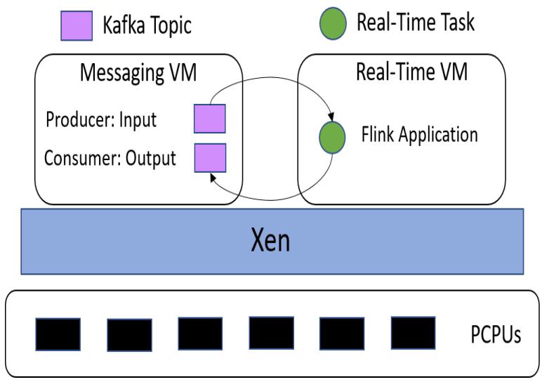 Fig. 3: Experimental Setup configured with Xen 4.10 as the hypervisor and Ubuntu 16.04 as the domain0 operating system. Each of the guest domains also run Ubuntu 16.04. Within the messaging VM, I created Kafka producers for each detector location for a total of six producers. I made one consumer for the output topic. Recall that Kafka also requires Apache Zookeeper to help coordinate services. Since I want to be able to pin each of these processes to a specific VCPU, the messaging VM requires eight cores. I allocated 16GB of memory to this machine since it will be responsible for running many services. Within the real-time VM, I will only run the Flink application. I allocate this VM only two cores and 8GB of memory. Flink Application The Flink application provides the workload whose latency I will empirically study. At initialization, the application loads the pre-trained LSTM neural network from memory and initializes a directed graph. The directed graph consists of nodes representing the detector locations and edges representing the freeways. As a source, the Flink application consumes from the Kafka input topic. Each record contains four fields: a detector location, average speed, traffic flow, and a timestamp. The average speed and traffic flows are both 12x1 vectors of the raw data at 5-minute intervals as captured by the detector. As soon as the application receives a new record, it parses this information and scales the measured flows into the range [0,1]. The application then feeds these scaled flows into the LSTM neural network and creates a prediction, which is immediately transformed back to its original scale. The application then uses this heuristic to run the $A^*$ search algorithm to find the optimal path between the El Segundo and Long Beach detectors. Finally, the application creates a new record of the following information: detector location, average speed, traffic flows, timestamp, predicted flow, and path returned by $A^*$. As a sink, the Flink application publishes these new records to the Kafka output topic. Latency Calculation It is well known that traditional timestamping methods, such as the C routine dogetimeofday(), are unreliable in virtual environments [6]. To remedy this issue, I created a custom Python module that utilizes timestampcounter scaling in order to measure time precisely. This module provides an API to read the current value of the timestamp counter into the ex: tax registers and return this value. Once I have this value, I can convert it into nanoseconds by dividing it by the clock frequency of the CPU, assuming the clock frequency is constant. To enforce a continual clock frequency, I change the power settings in the system's BIOS. Although the CPU can optimize its power consumption through different p-states (performance states) and minimize power consumption through c-states, these create variability in the clock frequency of the CPU. By disabling these features, I fix the clock frequency. In this case, I fixed the clock frequency to 2.1GHz. I implement highly precise latency calculations in the messaging VM using this method. Each producer calls the custom module just before sending the message and appends the nanosecond timestamp to the record. When the consumer receives a record, it has access to this original timestamp. Therefore, the consumer can call the custom module and timestamp as soon as it receives a new record; the difference between these two timestamps represents the application's latency in nanoseconds. ## V. EVALUATION I empirically evaluate the latency of the Flink application on each of the three schedulers within Xen. One experiment corresponds to sending 20,000 records through the Flink application and recording the latencies for a given configuration. Each of the six producers sends a message from their detector location once every 100ms. Although real-world data comes only every 5 minutes, I accelerate the rate in order to achieve a suitable workload. ### a) RTDS Recall that within the RTDS scheduler, each VM must specify a budget and a period. Given that producers are sending messages once every 100ms, I set the period of the real-time VM to 100ms. Initially, I provide the real-time VM with access to the entire PCPU—that is, I set the budget to be equal to the period of 100ms. An ECDF curve of this configuration is shown in Figure 4. I can also specify a budget less than the value of the period, effectively giving the real-time VM partial access to the CPU or a "partial CPU." The benefit of not consuming the entire period is that the system may reclaim idle clock cycles and improve overall efficiency. If I keep the period the same, then I can discover a budget that gives the same latency performance as if the real-time VM had exclusive access to the CPU. I do so by first allocating a very small budget and then incrementally increasing the budget until the ECDF curves overlap. In nearly all cases, the budget was smaller than the period, and the maximum latency of the partial-CPU experiments was greater than those of the full-CPU counterpart. Table 4 summarizes these results. When I set the budget to 777500, 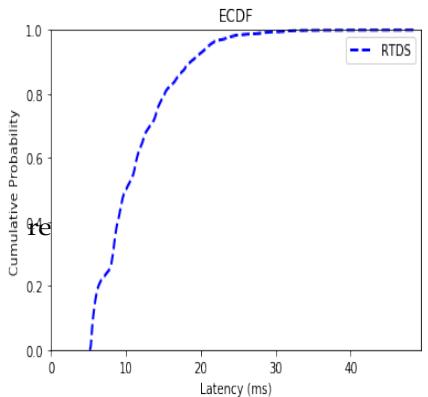 Fig. 4: ECDF of Latency Distribution RTDS Scheduler Table 4: Maximum Latencies for RTDS Experiments Scheduler Budget (μs) Period (μs) Maximum Latency (ms) <table><tr><td>Scheduler</td><td>Budget (μs)</td><td>Period (μs)</td><td>Maximum Latency (ms)</td></tr><tr><td>RTDS</td><td>100000</td><td>100000</td><td>48.52186857142857</td></tr><tr><td>RTDS</td><td>80000</td><td>100000</td><td>55.77778047619047</td></tr><tr><td>RTDS</td><td>77500</td><td>100000</td><td>38.0649180952381</td></tr><tr><td>RTDS</td><td>76750</td><td>100000</td><td>49.31550476190476</td></tr><tr><td>RTDS</td><td>76000</td><td>100000</td><td>61.50309523809524</td></tr><tr><td>RTDS</td><td>75000</td><td>100000</td><td>55.69025428571428</td></tr></table> I actually observed an improvement in the maximum latency observed. On the other hand, almost all of the partial-CPU experiments yielded ECDF curves that indicated a critical majority of the latencies were smaller than those of the full-CPU counterparts. Consider Figure 5, which shows the ECDF curves of the full-CPU and budget=77500 experiments. Not only does this experiment have a smaller maximum latency and, therefore, can provide a better service-level agreement, but the ECDF curve also lies above that of the full CPU experiment. This behavior is also exhibited in the other experiments with budgets greater than 76750. The experiment with the budget set to 76750 showed near equivalent performance both in terms of maximum latency, as seen in Table 4, but also with respect to their ECDF curves, as seen in Figure 6. 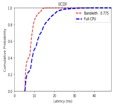 Fig. 5: ECDF Latency Distribution Partial CPU (0.775) vs. Full CPU RTDS Scheduler 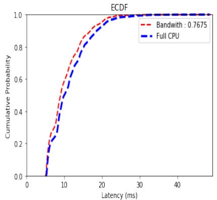 Fig. 6. ECDF Latency Distribution Partial CPU (0.7675) vs. Full CPU RTDS Scheduler ### b) Credit Under the default Credit scheduler, each VM can specify a weight and optional cap. The cap is expressed in terms of the number of VCPUs. While it is not a direct equivalence, I can vary the cap parameter for the real-time VM to achieve a similar effect as the partial CPU cases that were discussed with RTDS above. We, therefore, conduct two experiments: one without any caps and one with a cap. Recall that the partial-CPU experiment that was most similar to the full-CPU experiment using the RTDS scheduler had a budget of 76750 and a period of 100000. Therefore, since the real-time VM had two cores, it effectively made up of $\frac{76750}{100000} *2 = 153\%$ of a single PCPU. Because the cap parameter in Credit iCreditessed in terms of the percentage of CPUs, I set the cap of the real-time VM to be 153 for the partial-CPU Credit experiment. Table 5 Creditizes the experimental results. Figure 7 shows the ECDF curves for the full CPU experiments using Credit and RTDS schedulers. The full-CPU Credit scheduler distribution exhibits characteristics similar to those of the partial-CPU RTDS experiments. The majority of the Credit ECDF curve lies above that of the RTDS, and it has a higher maximum latency. Figure 8 shows the ECDF curves for the partial CPU experiments using Credit and RTDS schedulers. Observe that the green line corresponding to the Credit Partial CPU ECDF curve trails off of the plot. This is because the partial-CPU credit experiment's maximum latency was abysmally large—over a second. If the plot were to show the entire graph, the two curves would be indistinguishable, so I limit the X-axis for readability. Table 5: Maximum Latencies for Credit Experiments \\begin{table}[htbp] \\centering \\begin{tabular}{llc} \\hline Scheduler & Cap & Maximum Latency (ms) \\ \\hline Credit & 0 (None) & 116.94941476190476 \\Credit & 153 & 1040.939347142857 \\ \\hline \\end{tabular} \\end{table} <table> <tr> <td>Scheduler</td> <td>Cap</td> <td>Maximum Latency (ms)</td> </tr> <tr> <td>Credit</td> <td>0 (None)</td> <td>116.94941476190476</td> </tr> <tr> <td>Credit</td> <td>153</td> <td>1040.939347142857</td> </tr> </table> 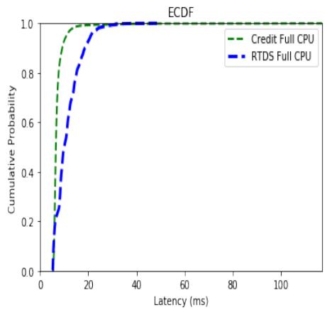 Fig. 7: ECDF Latency Distribution Full CPU Credit vs. Full CPU RTDS 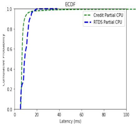 Fig. 8: ECDF Latency Distribution Partial CPU Credit vs. Partial CPU RTDS ### c) Credit2 Although Credit2 is the evolution of the Credit scheduler, it does not yet support a cap feature. As a result, I cannot run experiments that limit the CPU of a VM. We, therefore, only run one experiment, which is equivalent to the full-CPU scenarios described above. Table 6 summarizes the experimental results. Table 6: Maximum Latencies for Credi2t Experiments <table><tr><td>Scheduler</td><td>Maximum Latency (ms)</td></tr><tr><td>Credit2</td><td>951.1479685714286</td></tr></table> Credit2 suffered from the same behavior that was observed under the default credit scheduler—the maximum latency was tremendously large even though a significant portion of the records were processed faster than in RTDS. Figure 9 shows the ECDF curves for all three full-CPU experiments. Observe that I limited the X-axis of this plot for readability due to the same reasons discussed above: the large maximum latency would otherwise make the graphs indistinguishable. 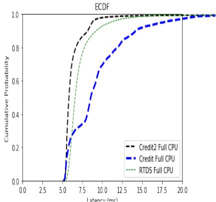 Fig. 9: ECDF Latency Distribution Full CPU Credit2 vs. Full CPU Credit vs. Full CPU RTDS It is readily apparent that the choice of hypervisor is largely dependent on the use case. For applications that require ultra-low-latency service level agreements, the RTDS scheduler is the clear choice. For other applications that are more concerned with median performance, the Credit and Credit2 schedulers seem to provide better performance. Although I artificially accelerated the input rate of the producers to achieve a more critical workload, this workload demonstrates the performance benefits and drawbacks of each scheduler. ## VI. CONCLUSION I have developed a model of an ITS that provides real-time optimal routing through the use of traffic forecasting. I have used this model as a workload to empirically study the effect that the choice of scheduler has on the latency of the application. It is evident from these experiments that the choice of scheduler largely depends on the application's use case. The RTDS scheduler provides excellent latency guarantees, whereas the Credit and Credit2 schedulers are more general-purpose. It is important to note that I have sacrificed a few real-world conditions in order to create a viable workload. First, I have statically defined the start and end locations for the $A^*$ search algorithm. In contrast, in the real world, they would certainly be more dynamic, and the network graph would be significantly larger in order to represent the roads and freeways of the surrounding area accurately. Additionally, I have artificially increased the rate of input in order to achieve a critical workload and demonstrate the effectiveness of the three schedulers. Although most cities do not currently have real-time traffic data, the advent of self-driving cars and other IoT devices has significant implications for the amount of data being transmitted and computed. This work creates several future research opportunities in a variety of different areas. It may be useful to examine the source code to understand better why the RTDS scheduler lacks some aspects of efficiency relative to Credit and Credit2. This work may also be extended to compare the effects of different architecture choices, such as the choice of a different messaging middleware. Lastly, although this work provides a basic model of an ITS with routing capabilities, there are many possible features to integrate into this model to make it more applicable to the real world.

Generating HTML Viewer...

References

17 Cites in Article
Paul Barham,Boris Dragovic,Keir Fraser,Steven Hand,Tim Harris,Alex Ho,Rolf Neugebauer,Ian Pratt,Andrew Warfield (2003). Xen and the art of virtualization.
Y Bengio,P Simard,P Frasconi (1994). Learning long-term dependencies with gradient descent is difficult.
Y Chen,M Guizani,Y Zhang,L Wang,N Crespi,G Lee (2017). When traffic flow prediction meets wireless big data analytics.
C Chong-White,G Millar,F Johnson,S Shaw (2011). The scats and the environment study: introduction and preliminary results.
I Corporation (2015). Timestamp-counter scaling (tsc scaling) for virtualization.
Shengdong Du,Tianrui Li,Xun Gong,Shi-Jinn Horng (2018). A Hybrid Method for Traffic Flow Forecasting Using Multimodal Deep Learning.
A Ferdowsi,U Challita,W Saad (2017). Deep learning for reliable mobile edge analytics in intelligent transportation systems.
Yann Lecun,Yoshua Bengio,Geoffrey Hinton (2015). Deep learning.
Yisheng Lv,Yanjie Duan,Wenwen Kang,Zhengxi Li,Fei-Yue Wang (2015). Traffic Flow Prediction With Big Data: A Deep Learning Approach.
Zhongjian Lv,Jiajie Xu,Kai Zheng,Hongzhi Yin,Pengpeng Zhao,Xiaofang Zhou (2018). LC-RNN: A Deep Learning Model for Traffic Speed Prediction.
S Maerivoet,B Moor (2005). Traffic flow theory.
Nicholas Polson,Vadim Sokolov (2015). Bayesian Particle Tracking of Traffic Flows.
N Polson,V Sokolov (2017). Deep learning for short-term traffic flow prediction.
A Sherstinsky (2018). Fundamentals of recurrent neural network (RNN) and long shortterm memory (LSTM) network.
N Srivastava,G Hinton,A Krizhevsky,I Sutskever,R Salakhutdinov (2014). Dropout: A simple way to prevent neural networks from overfitting.
B Williams,L Hoel (2003). Modeling and forecasting vehicular traffic flow as a seasonal arima process: Theoretical basis and empirical results.
Sisu Xi,Meng Xu,Chenyang Lu,Linh Phan,Christopher Gill,Oleg Sokolsky,Insup Lee (2014). Real-time multi-core virtual machine scheduling in xen.
No ethics committee approval was required for this article type.
Data Availability
Not applicable for this article.
How to Cite This Article
Azizul Hakim Rafi. 2026. \u201cOptimizing Real-Time Intelligent Traffic Systems with LSTM Forecasting and A* Search: An Evaluation of Hypervisor Schedulers\u201d. Global Journal of Computer Science and Technology - D: Neural & AI GJCST-D Volume 24 (GJCST Volume 24 Issue D2): .
Explore published articles in an immersive Augmented Reality environment. Our platform converts research papers into interactive 3D books, allowing readers to view and interact with content using AR and VR compatible devices.
Your published article is automatically converted into a realistic 3D book. Flip through pages and read research papers in a more engaging and interactive format.
This research explores an Intelligent Traffic System (ITS) designed for real-time optimal routing using traffic forecasting and an A* search algorithm. Leveraging a pre-trained Long Short-Term Memory (LSTM) neural network, I predict traffic flow based on historical data to inform heuristic functions, ensuring optimal route calculations. The heuristic is constructed to be permissible and consistent by incorporating predicted traffic flow and average speed measurements. The experimental setup involves a messaging virtual machine (VM) and a realtime VM within a Xen hypervisor environment, utilizing Apache Kafka and Apache Flink for data flow and processing. I empirically evaluate the latency performance of the ITS under three different Xen schedulers: RTDS, Credit, and Credit2. My findings indicate that the RTDS scheduler provides superior latency guarantees, making it suitable for applications requiring ultra-low latency, whereas the Credit and Credit2 schedulers offer better median performance. These insights highlight the impact of hypervisor scheduler choice on the efficiency and responsiveness of real-time ITS applications.
Our website is actively being updated, and changes may occur frequently. Please clear your browser cache if needed. For feedback or error reporting, please email [email protected]
Thank you for connecting with us. We will respond to you shortly.