## I. MAXWELL EQUATION IN GEOMETRIC ALGEBRA TO SIMULATE COMPUTING DEVICE OF ANALOG COMPUTER An analog computer is generally a type of computing device that uses the continuous variation aspect of physical phenomena to model the problem being solved[1]. One special type of physical phenomenon to model problems is considered below. The circular polarized electromagnetic waves following from the solution of Maxwell equations in free space done in geometric algebra terms,[^2], [3], are the electromagnetic fields of the form: $$ F = F _ {0} \exp \left[ I _ {S} (\omega t - k \cdot r) \right] \tag {1.1} $$ which should be the solution of $$ \left(\partial_ {t} + \nabla\right) F = 0 \tag {1.2} $$ Solution of (1.2) must be the sum of a vector (electric field $e$ ) and bivector (magnetic field $I_3h$ ): $$ F = e + I _ {3} h, $$ with some initial conditions: $$ e + I _ {3} h | _ {t = 0, \vec {r} = 0} = F _ {0} = e | _ {t = 0, \vec {r} = 0} + I _ {3} h | _ {t = 0, \vec {r} = 0} = e _ {0} + I _ {3} h _ {0} $$ For a given plane $S$ in (1.1), the solution of the three-dimensional Maxwell equation (1.2) has two options: - $F_{+} = (e_{0} + I_{3}h_{0})\exp [I_{S}(\omega t - k_{+}\cdot r)]$, with $\hat{k}_{+} = I_{3}I_{S},\hat{e}\hat{h}\hat{k}_{+} = I_{3}$, and the triple $\{\hat{e},\hat{h},\hat{k}_{+}\}$ is right hand screw oriented, that's rotation of $\hat{e}$ to $\hat{h}$ by $\pi /2$ gives movement of right hand screw in the direction of $k_{+} = k|I_3I_S$; - $F_{-} = (e_{0} + I_{3}h_{0})\exp [I_{S}(\omega t - k_{-}\cdot r)]$, with $\hat{k}_{-} = -I_{3}I_{S},\hat{e}\hat{h}\hat{k}_{-} = -I_{3}$, and the triple $\{\hat{e},\hat{h},\hat{k}_{-}\}$ is left hand screw oriented, that's the rotation of $\hat{e}$ to $\hat{h}$ by $\pi /2$ gives movement of left-hand screw in the direction of $k_{-} = -|k|I_{3}I_{S}$ or, equivalently, movement of right-hand screw in the opposite direction, $-k_{-}$; where $e_0$ and $h_0$, initial values of $e$ and $h$, are arbitrary mutually orthogonal vectors of equal length, lying on the plane $S$. Vectors $k_{\pm} = \pm |k_{\pm}|I_3I_S$ are normal to that plane. The length of the "wave vectors" $|k_{\pm}|$ is equal to angular frequency $\omega$. Maxwell's equation (1.2) is a linear one. Then, any linear combination of $F_{+}$ and $F_{-}$ saving the structure of (1.1) will also be a solution. Let's write: $$ \left\{ \begin{array}{l l} F _ {+} = (e _ {0} + I _ {3} h _ {0}) \exp [ I _ {S} \omega (t - (I _ {3} I _ {S}) \cdot r) ] = (e _ {0} + I _ {3} h _ {0}) \exp [ I _ {S} \omega t ] \exp [ - I _ {S} [ (I _ {3} I _ {S}) \cdot r ] ] \\ F _ {-} = (e _ {0} + I _ {3} h _ {0}) \exp [ I _ {S} \omega (t + (I _ {3} I _ {S}) \cdot r) ] = (e _ {0} + I _ {3} h _ {0}) \exp [ I _ {S} \omega t ] \exp [ I _ {S} [ (I _ {3} I _ {S}) \cdot r ] ] \end{array} \right. \tag {1.3} $$ Then, for arbitrary (real2) scalars $\lambda$ and $\mu$: $$ \lambda F _ {+} + \mu F _ {-} = (e _ {0} + I _ {3} h _ {0}) e ^ {I _ {S} \omega t} (\lambda e ^ {- I _ {S} [ (I _ {3} I _ {S}) \cdot r ]} + \mu e ^ {I _ {S} [ (I _ {3} I _ {S}) \cdot r ]}) \tag {1.4} $$ is also solution of (1.2). The item in the second parenthesis is a weighted linear combination of two states (wave functions, g-qubits[4], [5]) with the same phase in the same plane but the opposite sense of orientation. The states are strictly coupled, entangled if you prefer, because the bivector plane should be the same for both, no matter what happens with that plane. Arbitrary linear combination (1.4) can be rewritten as: $$ \lambda e ^ {I _ {\text{Plane}} ^ {+} \varphi^ {+}} + \mu e ^ {I _ {\text{Plane}} ^ {-} \varphi^ {-}} \tag{1.5}, $$ $$ \varphi^ {\pm} = \cos^ {- 1} \left(\frac {1}{\sqrt {2}} \cos \omega (t \mp [ (I _ {3} I _ {S}) \cdot r ])\right), $$ $$ \begin{array}{l} I _ {P l a n e} ^ {\pm} = I _ {S} \frac {s i n \omega (t \mp [ (I _ {3} I _ {S}) \cdot r ])}{\sqrt {1 + s i n ^ {2} \omega (t \mp [ (I _ {3} I _ {S}) \cdot r ])}} + I _ {B _ {0}} \frac {c o s \omega (t \mp [ (I _ {3} I _ {S}) \cdot r ])}{\sqrt {1 + s i n ^ {2} \omega (t \mp [ (I _ {3} I _ {S}) \cdot r ])}} \\+ I _ {E _ {0}} \frac {\sin \omega (t \mp [ (I _ {3} I _ {S}) \cdot r ])}{\sqrt {1 + \sin^ {2} \omega (t \mp [ (I _ {3} I _ {S}) \cdot r ])}} \\\end{array} $$ The triple of unit value basis orthonormal bivectors $\{I_S, I_{B_0}, I_{E_0}\}$ comprises the $I_S$ bivector, dual to the propagation direction vector; $I_{B_0}$ is dual to the initial vector of magnetic field; $I_{E_0}$ is dual to the initial vector of electric field. The expression (1.5) is a linear combination of two geometric algebra states, g-qubits. Linear combination of the two equally weighted solutions of the Maxwell equation $F_{+}$ and $F_{-}$, $\lambda F_{+} + \mu F_{-}$ with $\lambda = \mu = 1$ reads: $$ \lambda F_{+} + \mu F_{-}|_{\lambda=\mu=1} = 2 \cos \omega \left[ \left(I_{3} I_{S}\right) \cdot r \right] \left(\frac{1}{\sqrt{2}} \cos \omega t + I_{S} \frac{1}{\sqrt{2}} \sin \omega t + I_{B_{0}} \frac{1 }{\sqrt{2}} \cos \omega t + I_{E_{0}} \frac{1}{\sqrt{2}} \sin \omega t\right) \tag{1.6} $$ where $\cos \varphi = \frac{1}{\sqrt{2}}\cos \omega t$ and $\sin \varphi = \frac{1}{\sqrt{2}}\sqrt{1 + (\sin \omega t)^2}$. It can be written in standard exponential form $\cos \varphi + \sin \varphi I_B = e^{I_B\varphi}$.[^3] I will call such kind of g-qubits spreons (or sprefields.) They spread over the entire three-dimensional space for all values of time and, particularly, instantly change under Clifford translations over the whole three-dimensional space for all values of time, along with the results of measurement of any observable. ## II. CUDA GPU SIMULATION OF THE ANALOG MODELING COMPUTER In classical mechanics, states are identified by vectors in three-dimensional space [6]. Infinitesimal transformation of a state, vector, in classical mechanics is: $$ \vec {X} (t + \Delta t) \approx \vec {X} (t) + \frac {\partial}{\partial t} \vec {X} (t) \Delta t $$ $$ \frac {\vec {X} (t + \Delta t) - \vec {X} (t)}{\Delta t} \approx \frac {\partial}{\partial t} \vec {X} (t) $$ In our torsion mechanics [7] states, wave functions, are identified by points on three-sphere $\mathbb{S}^3$. A state[^4] there is, see[5], Sec.2.5: $$ e ^ {I _ {S} (t) \varphi (t)}, $$ where $I_S$ is a unit value bivector. If we take a Hamiltonian $H(t) = \alpha + I_3(\beta B_1 + \gamma B_2 + \delta B_3)$ in some orthogonal basis, see[^2], then for infinitesimal transformation we have: $$ e ^ {I _ {S} (t _ {0} + \Delta t) \varphi (t _ {0} + \Delta t)} = e ^ {- I _ {H} (t _ {0}) | H (t _ {0}) | \Delta t} e ^ {I _ {S} (t _ {0}) \varphi (t _ {0})} $$ and $$ \begin{array}{l} \lim _ {\Delta t \to 0} \frac{\Delta e ^ {I _ {S} (t _ {0}) \varphi (t _ {0})}}{\Delta t} = \lim _ {\Delta t \to 0} \frac{e ^ {I _ {S} (t _ {0} + \Delta t) \varphi (t _ {0} + \Delta t)} - e ^ {I _ {S} (t _ {0}) \varphi (t _ {0})}}{\Delta t} \\= \lim _ {\Delta t \to 0} \frac{(1 - I _ {H} (t _ {0}) | H (t _ {0}) | \Delta t) e ^ {I _ {S} (t _ {0}) \varphi (t _ {0})} - e ^ {I _ {S} (t _ {0}) \varphi (t _ {0})}}{\Delta t} \\= - I _ {H} (t _ {0}) | H (t _ {0}) | e ^ {I _ {S} (t _ {0}) \varphi (t _ {0})} \\\end{array} $$ We received the Schrodinger equation for the state $e^{I_S(t)\varphi (t)}$. That means that the Schrodinger equation governs the evolution of operators, states, which act on observables. While in classical mechanics, measurement of observable $\vec{x}(t)$ (action by a state) is a shift by a state: $$ \vec {x} (t) \rightarrow \vec {x} (t) + \vec {X} (t), $$ in the torsion mechanics it is: $$ C \rightarrow e ^ {- I _ {S} (t) \varphi (t)} C e ^ {I _ {S} (t) \varphi (t)}, $$ that's rotation in the plane of bivector $I_{S}$ by angle $\varphi$. Take the general case of observable as a g-qubit: $C = C_0 + C_1B_1 + C_2B_2 + C_3B_3$. Its measurement by a state $\alpha + \beta_1B_1 + \beta_2B_2 + \beta_3B_3$ is [4]: $$ \begin{array}{l} C _ {0} + C _ {1} B _ {1} + C _ {2} B _ {2} + C _ {3} B _ {3} \xrightarrow {\alpha + \beta_ {1} B _ {1} + \beta_ {2} B _ {2} + \beta_ {3} B _ {3}} C _ {0}: \\+ \left(C _ {1} [ (\alpha^ {2} + \beta_ {1} ^ {2}) - (\beta_ {2} ^ {2} + \beta_ {3} ^ {2}) ] + 2 C _ {2} (\beta_ {1} \beta_ {2} - \alpha \beta_ {3}) + 2 C _ {3} (\alpha \beta_ {2} + \beta_ {1} \beta_ {3})\right) B _ {1} \\+ \left(2 C _ {1} (\alpha \beta_ {3} + \beta_ {1} \beta_ {2}) + C _ {2} [ (\alpha^ {2} + \beta_ {2} ^ {2}) - (\beta_ {1} ^ {2} + \beta_ {3} ^ {2}) ] + 2 C _ {3} (\beta_ {2} \beta_ {3} - \alpha \beta_ {1})\right) B _ {2} \\+ (2 C _ {1} (\beta_ {1} \beta_ {3} - \alpha \beta_ {2}) + 2 C _ {2} (\alpha \beta_ {1} + \beta_ {2} \beta_ {3}) + C _ {3} [ (\alpha^ {2} + \beta_ {3} ^ {2}) - (\beta_ {1} ^ {2} + \beta_ {2} ^ {2}) ]) B _ {3} \\\end{array} $$ When the state is (1.6) we have: $$ B_{1} = I_{S},\quad B_{2} = I_{B_{0}},\quad B_{3} = I_{E_{0}},\quad \alpha = 2\cos\omega\left[(I_{3}I_{S})\cdot r\right]\frac{1}{\sqrt{2}}\cos\omega t,\quad \beta_{1} = 2\cos\omega\left[(I_{3}I_{ ext{S}})\cdot r\right]\frac{\sqrt{2}}{r}. $$ $$ r ] \frac {1}{\sqrt {2}} \sin \omega t, \beta_ {2} = 2 \cos \omega [ (I _ {3} I _ {S}) \cdot r ] \frac {1}{\sqrt {2}} \cos \omega t, \beta_ {3} = 2 \cos \omega [ (I _ {3} I _ {S}) \cdot r ] \frac {1}{\sqrt {2}} \sin \omega t $$ And the measurement result is $G_3^+$ element spreading through the three-dimensional space for all values of time parameter $t$: $$ 4 \cos^ {2} \omega \left[ \left(I _ {3} I _ {S}\right) \cdot r \right] \left[ C _ {0} + C _ {3} I _ {S} + \left(C _ {1} \sin 2 \omega t + C _ {2} \cos 2 \omega t\right) I _ {B _ {0}} + \left(C _ {2} \sin 2 \omega t - C _ {1} \cos 2 \omega t\right) I _ {E _ {0}} \right] \tag {2.1} $$ Geometrically, that means that the measured observable is rotated by $\frac{\pi}{2}$ in the $I_{B_0}$ plane, such that the $C_3I_S$ component becomes orthogonal to plane $I_S$ and remains unchanged. Two other components became orthogonal to $I_{B_0}$ and $I_{E_0}$ and continue rotating in $I_S$ with angular velocity $2\omega t$. The factor $4\cos^2\omega [(I_3I_S)\cdot r]$ defines the dependency of that transformed values through all points of the three-dimensional space. The hardware creating sprefields may require special implementation as a photonic/laser device that does not exist yet. Instead, we have a very convenient equivalent simulation scheme where the amount of simultaneously available space/time points of observable measured values is only restricted by the overall available Nvidia GPU number of threads. The case of measuring $C = C_0 + C_1B_1 + C_2B_2 + C_3B_3$ by the sprefield is processed by using the following kernel function in the CUDA code: {"algorithm_caption":[],"algorithm_content":[{"type":"text","content":"__global__ void quant Kernel(float4\\* output, int dimx, int dimy, int dimz, float t) \n{\nfloatC1 "},{"type":"equation_inline","content":"= 1.0 / /"},{"type":"text","content":" optional components of the observable \nfloatC2 "},{"type":"equation_inline","content":"= 1.0"},{"type":"text","content":". \nfloatC3 "},{"type":"equation_inline","content":"= 1.0"},{"type":"text","content":". \nfloat omega "},{"type":"equation_inline","content":"= 12560000.0"},{"type":"text","content":" // variant of angular velocity in the sprefield \nfloat tstep "},{"type":"equation_inline","content":"= 1.0f"},{"type":"text","content":".. \nfloat factor "},{"type":"equation_inline","content":"= 0.0"}]} {"code_caption":[],"code_content":[{"type":"text","content":"int qidx = threadIdx.x + blockIdx.x * blockDim.x; \nint qidy = threadIdx.y + blockIdx.y * blockDim.y; \nint qidz = threadIdx.z + blockIdx.z * blockDim.z; \nsize`t oidx = qidx + qidy*dimx + qidz*dimx*dimy; \noutput[oidx][0] = oidx*tstep; \nfactor = 4*(cosf(omega * output[oidx][0])) * (cosf(omega * output[oidx][0])); \noutput[oidx][0] += factor * C3; \noutput[oidx][1] = oidx*tstep; \noutput[oidx][1] += factor * (C1sin(2*omega*t) + C2cos(2*omega*t)); \noutput[oidx][^2] = oidx*tstep; \noutput[oidx][^2] += factor * (C2sin(2*omega*t) - C1cos(2*omega*t)); \noutput[oidx][3] = factor; \n} "}],"code_language":"lisp"} More flexibility can be achieved by scattering the sprefield wave function before applying it to observables. Arbitrary Clifford translation $e^{I_{B_C}\gamma} = \cos \gamma + \sin \gamma \left( \gamma_1 I_S + \gamma_2 I_{B_0} + \gamma_3 I_{E_0} \right)$ acting on spreons (1.6) gives: $$ 2\cos\omega\left[(I_3I_S)\cdot r\right]\left[\frac{1}{\sqrt{2}}(\cos\gamma\cos\omega t-\gamma_1\sin\gamma\sin\omega t-\gamma_2\sin\gamma\cos\omega t-\gamma_3\sin\gamma\sin\omega t) + \frac{1}{\sqrt{2}}(\cos\gamma\sin\omega t+\gamma_1\sin\gamma\cos\omega t-\gamma_2\sin\gamma\sin\omega t+\gamma_3\sin\gamma\cos\omega t)I_S + \frac{1}{\sqrt{2}}(\cos\gamma\cos\omega t+\gamma_1\sin\gamma\sin\omega t+\gamma_2\sin\gamma\cos\omega t-\gamma_3\sin\gamma\sin\omega t)I_{B_0} + \frac{1}{\sqrt{2}}(\cos\gamma\sin\omega t-\gamma_1\sin\gamma\cos\omega t+\gamma_2\sin\gamma\sin\omega t+\gamma_3\sin\gamma\cos\omega t)I_{E_0}\right]\tag{2.2} \end{array} $$ This result is defined for all values of $t$ and $r$, in other words, the effect of Clifford translation instantly spreads through the whole three dimensions for all values of the time. The instant of time when the Clifford translation was applied makes no difference for the state (2.2) because it is simultaneously redefined for all values of $t$. The values of measurements $O\left(C_0, C_1, C_2, C_3, I_S, I_{B_0}, I_{E_0}, \gamma, \gamma_1, \gamma_2, \gamma_3, \omega, t, r\right)$ also get instantly changed for all values of time of measurement, even if the Clifford translation was applied later than the measurement. That is an obvious demonstration that the suggested theory allows indefinite event casual order. In that way, the very notion of the concept of cause and effect, ordered by time value increasing, disappears. The result of the measurement in general case is a bit tedious. Let us take as an example the bivector components with $\gamma_{2} = 1$, $\gamma_{1} = \gamma_{3} = 0$. In that case, the result of measurement of $C_0 + C_1I_S + C_2I_{B_0} + C_3I_{E_0}$ can be calculated as its measurement by $\cos \gamma + \sin \gamma I_{B_0}$: $$ C_0 + C_1 I_S + C_2 I_{B_0} + C_3 I_{E_0} \xrightarrow{\cos\gamma + \sin\gamma I_{B_0}} C_0 + (C_1 \cos 2\gamma + C_3 \sin 2\gamma) I_S + C_2 I_{B_0} + (C_3 \cos 2\gamma - C_1 \sin 2\gamma) I_{E_0} $$ followed by measurement by $$ \begin{array}{l} 4 (\cos \omega [ (I _ {3} I _ {S}) \cdot \vec {r} ]) ^ {2} \big [ C _ {0} + (C _ {3} \cos 2 \gamma - C _ {1} \sin 2 \gamma) \big (\cos 2 \gamma I _ {S} - \sin 2 \gamma I _ {E _ {0}} \big) \\+ \left(\left(C _ {1} \cos 2 \gamma + C _ {3} \sin 2 \gamma\right) \sin 2 \omega t + C _ {2} \cos 2 \omega t\right) I _ {B _ {0}} \\+ \left(C _ {2} \sin 2 \omega t - \left(C _ {1} \cos 2 \gamma + C _ {3} \sin 2 \gamma\right) \cos 2 \omega t\right) \left(\cos 2 \gamma I _ {E _ {0}} + \sin 2 \gamma I _ {S}\right) \Big ] \\\end{array} $$ If we take the new orthonormal bivector basis: $$ \left\{\cos 2 \gamma I _ {S} - \sin 2 \gamma I _ {E _ {0}}, \sin 2 \gamma I _ {S} + \cos 2 \gamma I _ {E _ {0}}, \quad I _ {B _ {0}} \big \} \equiv \left\{I _ {1 \gamma}, I _ {2 \gamma}, I _ {B _ {0}} \right\} $$ the result of the measurement reads: $$ \begin{array}{l} 4 (\cos \omega [ (I _ {3} I _ {S}) \cdot \vec {r} ]) ^ {2} \bigl [ C _ {0} + (C _ {3} \cos 2 \gamma - C _ {1} \sin 2 \gamma) I _ {1 \gamma} \\+ \left(\left(C _ {1} \cos 2 \gamma + C _ {3} \sin 2 \gamma\right) \sin 2 \omega t + C _ {2} \cos 2 \omega t\right) I _ {B _ {0}} \\\left. + \left(C _ {2} \sin 2 \omega t - \left(C _ {1} \cos 2 \gamma + C _ {3} \sin 2 \gamma\right) \cos 2 \omega t\right) I _ {2 \gamma} \right] \\\end{array} $$ Notes that has constant value in plane $I_{1\gamma}$ plus rotation in planes $I_{B_0}$ and $I_{2\gamma}$ with angular velocity $2\omega$. In that way, we can get an $\vec{r}$ -dependent variety of constant components of the results of measurements: $$ 4 (\cos \omega [ (I _ {3} I _ {S}) \cdot \vec {r} ]) ^ {2} \big [ C _ {0} + (C _ {3} \cos 2 \gamma - C _ {1} \sin 2 \gamma) \big (\cos 2 \gamma I _ {S} - \sin 2 \gamma I _ {E _ {0}} \big) \big ] $$ ## III. EXAMPLES OF APPLICATIONS OF THE GPU SIMULATING QUANTUM COMPUTER ### a) Circulation of flow of a fluid Assume that fluid in 3D is a field of point-dependent values of vector field $\vec{v}(P)$. Consider a volume element $\tau$ containing within it a point $P$, and denote the bounding surface of $\tau$ by $\sigma$. Then, the flux of $\vec{v}$ over $\sigma$ per unit volume is $$ \frac {\int \vec {v} \cdot \vec {n} d \sigma}{\tau} $$ where the integral is taken over the surface $\sigma$ and $\vec{n}$ is the exterior unit normal to $\sigma$. Similarly, we can define: $$ c u r l \vec {v} (P) = \lim _ {\tau \rightarrow 0} \frac {\int \vec {v} \times \vec {n} d \sigma}{\tau} $$ Let $C$ is simple closed curve bounding a plane area $A$. At a given point $P$ of $A$ construct unit normal $\vec{\nu}$ so directed that $\vec{\nu}$ points in the direction of an advancing right-hand screw when $C$ is traversed in the positive sense. Take $\tau$ as a cylinder with base $A$ and a small height parallel to $\vec{v}$. The cylinder surface is $\sigma$. The definition of $\operatorname{curl} \vec{v}(P)$ yields: $$ \vec {v} \cdot c u r l \vec {v} (P) = \lim _ {\tau \rightarrow 0} \frac {\int \vec {v} \cdot \vec {v} \times \vec {n} d \sigma}{\tau} = \lim _ {A \rightarrow 0} \frac {\int \vec {v} \cdot d \vec {r}}{A} $$ where the second integral is along the curve $C$, and $d\vec{r}$ is the differential of the position vector on $C$. The line integral $\int \vec{v} \cdot d\vec{r}$ is called the circulation of $\vec{v}$ along $C$. If $\vec{v}$ represents the velocity of a fluid, then $\vec{v} \cdot d\vec{r}$ takes account of the tangential component of velocity $\vec{v}$ and, a fluid particle moving with this velocity circulates along $C$. A particle moving with velocity $\vec{v} \cdot \vec{n}$ normal to $C$, on the other hand, crosses $C$. That is, it flows either into or out of the region bounded by $C$. Hence $\vec{v} \cdot \text{curl} \, \vec{v}(P)$ provides a measure of the circulation per unit area at point $P$. Suppose a fluid is given in a three-dimensional region by continuously differential vector field $\vec{v}(P)$, the fluid velocity. At every point $P$ we have a value $\text{curl} \, \vec{v}(P)$ that can be identified by $C = C_0 + C_1 B_1 + C_2 B_2 + C_3 B_3 \equiv R e^{I_S(t) \varphi(t)}$ with geometrically known entities[^2]-[5]. The $\text{curl} \, \vec{v}(P)$ is the infinitesimal volume density of the net vector circulation, that is magnitude and spatial orientation of the field around the point. Let us apply the spreon (1.6) to the curl $\vec{v}(P)$ at some point $P$. According to (2.1), the result is: $$ \begin{array}{l} 4 R \cos^ {2} \omega \left[ \left(I _ {3} I _ {S}\right) \cdot r \right] \left[ C _ {0} + C _ {3} I _ {S} + \left(C _ {1} \sin 2 \omega t + C _ {2} \cos 2 \omega t\right) I _ {B _ {0}} \right. \\\left. + \left(C _ {2} \sin 2 \omega t - C _ {1} \cos 2 \omega t\right) I _ {E _ {0}} \right] \\\end{array} $$ In the current scheme any number of test observables can be placed into the continuum of the $(t, r^{\rightarrow})$ dependent values of the spreon state, thus fetching out any amount of values $O\big(C_0, C_1, C_2, C_3, I_S, I_{B_0}, I_{E_0}, \gamma, \gamma_1, \gamma_2, \gamma_3, \omega, t, r\big)$ spread over three-dimensions and at all instants of time not generally following cause/effect ordering[8]. While the Schrodinger equation governs infinitesimal transformations of a wave function by Clifford translations, a finite Clifford translation moves a wave function along a big circle of $\mathbb{S}^3$ by any Clifford parameter. In $G_3^+$ multiplication is: $$ g _ {1} g _ {2} = \big (\alpha_ {1} + I _ {S _ {1}} \beta_ {1} \big) \big (\alpha_ {2} + I _ {S _ {2}} \beta_ {2} \big) = \alpha_ {1} \alpha_ {2} + I _ {S _ {1}} \alpha_ {2} \beta_ {1} + I _ {S _ {2}} \alpha_ {1} \beta_ {2} + I _ {S _ {1}} I _ {S _ {2}} \beta_ {1} \beta_ {2} $$ It is not commutative due to the not commutative product of bivectors $I_{S_1}I_{S_2}$. Indeed, taking vectors to which $I_{S_1}$ and $I_{S_2}$ are dual: $s_1 = -I_3I_{S_1}$, $s_2 = -I_3I_{S_2}$, we have: $$ I _ {S _ {1}} I _ {S _ {2}} = - s _ {1} \cdot s _ {2} - I _ {3} (s _ {1} \times s _ {2}) $$ Then: $$ g _ {1} g _ {2} = \alpha_ {1} \alpha_ {2} - (s _ {1} \cdot s _ {2}) \beta_ {1} \beta_ {2} + I _ {S _ {1}} \alpha_ {2} \beta_ {1} + I _ {S _ {2}} \alpha_ {1} \beta_ {2} - I _ {3} (s _ {1} \times s _ {2}) \beta_ {1} \beta_ {2} $$ $$ g _ {2} g _ {1} = \alpha_ {1} \alpha_ {2} - (s _ {1} \cdot s _ {2}) \beta_ {1} \beta_ {2} + I _ {S _ {1}} \alpha_ {2} \beta_ {1} + I _ {S _ {2}} \alpha_ {1} \beta_ {2} + I _ {3} (s _ {1} \times s _ {2}) \beta_ {1} \beta_ {2} $$ I the case when both elements are of exponent form: $$ e^{I_{S_1} \varphi_1} = \alpha_1 + I_{S_1} \beta_1 = \alpha_1 + \beta_1 b_1^1 B_1 + \beta_1 b_1^2 B_2 + \beta_1 b_1^3 B_3 $$ $$ e^{I_{S_2} \varphi_2} = \alpha_2 + I_{S_2} \beta_2 = \alpha_2 + \beta_2 b_2^1 B_1 + \beta_2 b_2^2 B_2 + \beta_2 b_2^3 B_3, $$ $$ (\alpha_ {1}) ^ {2} + (\beta_ {1}) ^ {2} ((b _ {1} ^ {1}) ^ {2} + (b _ {1} ^ {2}) ^ {2} + (b _ {1} ^ {3}) ^ {2}) = (\alpha_ {1}) ^ {2} + (\beta_ {1}) ^ {2} = 1 $$ $$ (\alpha_ {2}) ^ {2} + (\beta_ {2}) ^ {2} ((b _ {2} ^ {1}) ^ {2} + (b _ {2} ^ {2}) ^ {2} + (b _ {2} ^ {3}) ^ {2}) = (\alpha_ {2}) ^ {2} + (\beta_ {2}) ^ {2} = 1, $$ as in the case of a wave function and Clifford translation, we get: $$ \begin{array}{l} e ^ {I _ {S _ {2}} \varphi_ {2}} e ^ {I _ {S _ {1}} \varphi_ {1}} = c o s \varphi_ {1} c o s \varphi_ {2} + (s _ {1} \cdot s _ {2}) s i n \varphi_ {1} s i n \varphi_ {2} + I _ {3} s _ {2} c o s \varphi_ {1} s i n \varphi_ {2} + I _ {3} s _ {1} c o s \varphi_ {2} s i n \varphi_ {1} \\- I _ {3} \left(s _ {2} \times s _ {1}\right) \sin \varphi_ {1} \sin \varphi_ {2} \\\end{array} $$ Then it follows that two wave functions are, in any case, connected by the Clifford translation: $$ e ^ {I _ {S _ {2}} \varphi_ {2}} = (e ^ {I _ {S _ {2}} \varphi_ {2}} e ^ {- I _ {S _ {1}} \varphi_ {1}}) e ^ {I _ {S _ {1}} \varphi_ {1}} \equiv C l (S _ {2}, \varphi_ {2}, S _ {1}, \varphi_ {1}) e ^ {I _ {S _ {1}} \varphi_ {1}}, $$ where $$ Cl(S_2,\varphi_2,S_1,\varphi_1) \equiv e^{I_{S_2}\varphi_2} e^{-I_{S_1}\varphi_1} = cos\varphi_1 cos\varphi_2 + (s_1\cdot s_2) sin\varphi_1 sin\varphi_2 + I_3 s_2 cos\varphi_1 sin\varphi_2 + I_3 s_1 cos\varphi_2 sin\varphi_1 + I_3 (s_2\times s_1) sin\varphi_1 sin\varphi_2. $$ From knowing Clifford translation connecting any two wave functions as points on $\mathbb{S}^3$, it follows that the result of measurement of any observable $C$ by wave function $e^{I_{S_1}\varphi_1}$, for example, $e^{-I_{S_1}\varphi_1}C e^{I_{S_1}\varphi_1} \equiv C(S_1,\varphi_1)$, immediately gives the result of (not made) measurement by $e^{I_{S_2}\varphi_2}$: $$ \begin{array}{l} e ^ {- I _ {S _ {2}} \varphi_ {2}} C e ^ {I _ {S _ {2}} \varphi_ {2}} = e ^ {- I _ {S _ {2}} \varphi_ {2}} e ^ {I _ {S _ {1}} \varphi_ {1}} e ^ {- I _ {S _ {1}} \varphi_ {1}} C e ^ {I _ {S _ {1}} \varphi_ {1}} e ^ {- I _ {S _ {1}} \varphi_ {1}} e ^ {I _ {S _ {2}} \varphi_ {2}} = e ^ {- I _ {S _ {2}} \varphi_ {2}} e ^ {I _ {S _ {1}} \varphi_ {1}} C (S _ {1}, \varphi_ {1}) e ^ {- I _ {S _ {1}} \varphi_ {1}} e ^ {I _ {S _ {2}} \varphi_ {2}} \\= C l (S _ {2}, - \varphi_ {2}, S _ {1}, - \varphi_ {1}) C (S _ {1}, \varphi_ {1}) \overline {{C l (S _ {2} , - \varphi_ {2} , S _ {1} , - \varphi_ {1})}} \\\end{array} $$ When assuming observables are also identified by points on $\mathbb{S}^3$ and thus are connected by formulas as the above one, we get that measurements of any amount of observables by arbitrary set of wave functions are simultaneously available. ### b) Application to block chain schemes Let us briefly consider the basics of how the block chain scheme generally works in the suggested spreon formalism.  Take a block of transactions stored at some value of time: The next block is assumed to include transaction Trnsct\`q1 of the part of the measurement result of the observable $C_0 + C_1B_1 + C_2B_2 + C_3B_3$ by the state, that is Clifford translation by $\cos \gamma + I_{B_0} \sin \gamma$ of the spreon $$ 2 \cos \omega ([ (I _ {3} I _ {S}) \cdot \vec {r} ]) \left(\frac {1}{\sqrt {2}} \cos \omega t + \frac {1}{\sqrt {2}} I _ {S} \sin \omega t + \frac {1}{\sqrt {2}} I _ {B _ {0}} \cos \omega t + \frac {1}{\sqrt {2}} I _ {E _ {0}} \sin \omega t\right), $$ namely, the part which exists and is constant for all values of time before the transaction and after the transaction. The transaction is a set of elements of $G_3^+$. The hypothetical quantum channel should transfer sequences of such elements, comprised of factors $4(cos \omega [(I_3I_S)\cdot \vec{r_n}])^2$ with predefined values of $\vec{r_n}$ sufficient for enough information about the result of measurement; scalar values $C_3$ and $C_1$ of the observable; basis bivectors $I_S$ and $I_{E_0}$; scalar $\gamma$ used in creating of a state which acted on the observable, along with the length of wave vector $|k| = \omega$. Since Trnsct_q1 exists for all values of time it will be automatically included in all previous blocks and in all blocks transacted in the future.  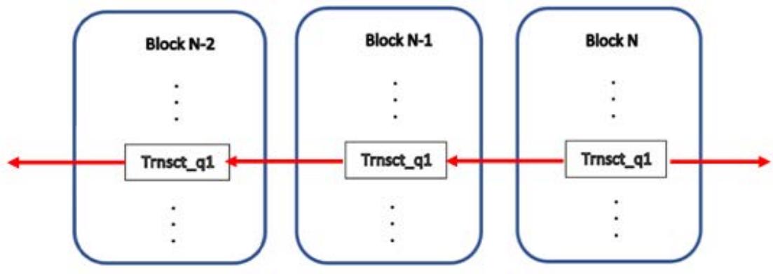When in future transactions of observable measurement result is transferred, new Trnsct_q2 is placed in all blocks in the same way as above for Trnsct_q1. ## IV. CONCLUSIONS In the suggested theory, all measured observable values get available all together, not through looking one by one. In this way, quantum computer appeared to be a kind of analog computer, keeping and instantly processing information by and on sets of objects possessing an infinite number of degrees of freedom. The multithread GPUs with the CUDA language functionality allow to simultaneously calculate observable measurement values at a number of space/time discrete points, forward and backward in time, the number only restricted by the GPU threads capacity. That eliminates the challenging hardware problem of creating vast and stable arrays of qubits, the basis of quantum computing in conventional approaches. [^2]: cos $\omega ([(I_3I_S)\cdot \vec{r} ])\left(\frac{1}{\sqrt{2}}\cos \omega t + \frac{1}{\sqrt{2}} I_S\sin \omega t + \frac{1}{\sqrt{2}} I_{B_0}\cos \omega t + \frac{1}{\sqrt{2}} I_{E_0}\sin \omega t\right)$ that gives: _(p.6)_

Generating HTML Viewer...

References

8 Cites in Article
Bernd Ulmann (2022). Analog Computing.
A Soiguine (2019). Instantaneous Spreading of the g-Qubit Fields.
Alexander Soiguine (2020). Scattering of Geometric Algebra Wave Functions and Collapse in Measurements.
Alexander Soiguine (2015). Explaining Some Weird Quantum Mechanical Features in Geometric Algebra Formalism.
Alexander Soiguine (2020). The Geometric Algebra Lift of Qubits and Beyond.
V Arnold (1989). Mathematical Methods of Classical Mechanics.
A Soiguine (2023). The Torsion Mechanics.
A Soiguine Parallelizable Computing with Geometric Algebra (Alternative to quantum computing based on entanglement).
No ethics committee approval was required for this article type.
Data Availability
Not applicable for this article.
How to Cite This Article
Alexander Soiguine. 2026. \u201cQuantum Computer as Analog Computer on GPU\u201d. Global Journal of Science Frontier Research - F: Mathematics & Decision GJSFR-F Volume 23 (GJSFR Volume 23 Issue F7).
Explore published articles in an immersive Augmented Reality environment. Our platform converts research papers into interactive 3D books, allowing readers to view and interact with content using AR and VR compatible devices.
Your published article is automatically converted into a realistic 3D book. Flip through pages and read research papers in a more engaging and interactive format.
Our website is actively being updated, and changes may occur frequently. Please clear your browser cache if needed. For feedback or error reporting, please email [email protected]
Thank you for connecting with us. We will respond to you shortly.