

I. INTRODUCTION
In a radio link over perfect ground traditionally two antennas are used for calibration of antenna factors. Independent of distance parameters of a receiving antenna are the effective length or effective height as well the antenna factor . These specific parameters depend only on the current distribution along the antenna physical structure. Other parameters like effective area and gain g are strongly dependent of the antenna location and precisely in the free space far field over ground.
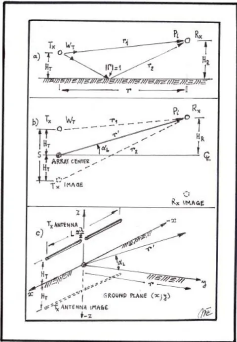
This condition is obtained when the wave impedance achieves the value of . The wave impedance is the relation between the electric and magnetic fields. Also, over perfect ground it depends, on the transmitting antenna radiation pattern elevation angle and distance r over ground between both antennas. This condition is not achieved at a fixed distance r but at a different distance depending by the corresponding radiation at any angle . This condition is achieved at a shorter distance when the maximum radiation is obtained by the transmitting antenna. is the distance along a straight line of an elevation angle departing from the ground plane shown in Figure 1. This point is the radiation phase center of the transmitting antenna. This distance is not obtained by a simple task but nowadays it can be determined by an antenna software [13]. This way the far field condition can be obtained and verifying it if at standard distances r the task is fulfilled [17].
At the same time, it is important to know that the wave power density flows in space travelling along the straight line between the radio link antennas [16]. In the radio link in free space the distance is exactly equal to the distance r if both antennas are identical. The transmitting antenna works over perfect ground with its image under ground and constitutes an array of two elements [2]. Its radiation pattern depends on the separation S between them, exactly like a two element array works in free space. For this reason for horizontal polarization the maximum radiation has an elevation angle according to this separation S or its height over ground and a null of power density on the perfect ground. Over ground this separacion is . Figure 1 shows a sketch of a transmitting antenna over perfect ground. Rx antenna receives the EM waves from the actual antenna and its image and it delivers the received power on only its load resistance and no EM waves are received on its image. This statement is very important. This way the Rx antenna in its receiving role is working like in free space even if it is working over perfect ground [2],[3],[17].
II. CALCULATION
The transmitting antenna (half-wave dipole) has a radiation pattern over perfect ground permitting to calculate its gain (dBi) for horizontal polarization. The original Dr. Kraus electric field gain equation over perfect ground is being updated to provide the power gain in dBi as a function of antenna height for various elevation angles of the radiating element, to be [2]:
Where:
2.15dBi is the half wave dipole antenna gain over an isotropic source in dB.
F is a factor taking into account the radiation resistance in free space and over perfect ground, or:
Tx antenna radiation resistance in free space. Tx antenna radiation resistance over perfect ground.
is the mutual resistance between Tx antenna and its image.
is the space phase constant [Rad/m] or .
is the transmitting antenna height over perfect ground [m].
is the elevation angle over ground from the array center phase located in the ground plane.
is the distance between the array phase center and the receiving antenna center over ground.
You may use this simple equation to calculate the gain radiation pattern of a very thin half wave dipole antenna at any height and obtain the far field gain. However, for more data result for this antenna at any frequency the aid of a software program will help reduce the tediousness of individual calculation to generate the radio link geometry for the specific antenna parameters [13]. These parameters are: the input antenna impedance, the current distribution on the antenna structure, the electric and magnetic fields, the power density on the location of the Rx antenna in space over ground, as well the gain radiation pattern in dBi in the far field. From the electric and magnetic field relation the wave impedance is determined at a specific location in space. Also from the radiation pattern the antenna gain in the far field for any elevation angle is obtained [13].
This procedure is performed easily at any frequency in the wanted spectrum.
Here an example at the frequency of f = 30 [MHz] is shown.
A radio link has two horizontally polarized half-wave dipole antennas as recommended by the Standard ANSI-IEEE C 63-5-2017 [18].
Tx antenna is resonant with a radiation resistance:
Tx antenna height .
Rx receiving antenna is located at a distance r = 10[m].
Results:
Tx antenna power input [W], [0 dBW].
Tx antenna length at resonance for a radius .
Tx antenna height over ground [m].
Tx antenna input resistance in resonance. Distance between antennas measured on the ground plane r = 10 [m].
Tx antenna radiation elevation angle [°].
Rx antenna height for relative maximum power density or field . Maximum Rx antenna height available.
Electric field [V/m], (-4.11 [dBV/m]).
Magnetic field [A/m].
Power density [W/m2].
Wave impedance .
True Tx antenna numerical gain .
True Tx antenna gain [dBi].
True Tx antenna gain [dBi].
Rx antenna effective length .
Distance between Tx center phase and Rx antenna center .
Rx antenna induced voltage [V].
Rx antenna current [A].
Rx antenna receiving voltage [V].
Rx antenna receiving power [W].
Radio link transmission loss or site attenuation [dB] [4], [10].
Free space loss [dB] [1]. Loss Relationship [dB][14]. Rx antenna effective area [6]. Rx antenna numerical gain . Rx antenna gain [dBi]. Rx antenna gain [dBi]. Friis equation gain, Tx antenna gain check [1]. [dBi](Friis Power Budget fulfilled). Rx antenna factor [1/m]. Rx antenna factor [dB/m]. Rx antenna factor [dB/m]. Tx antenna factor [1/m]. Tx antenna factor [dB/m]. Tx antenna factor [dB/m]. Normalized Site Attenuation NSA = [dB]. NSA = 18.70 - (-2.4) - (-2.02) = 23.12 [dB].
Using the equation [7] of Standard C 63-5-2004, [18]. the result is found to be:
The result is exactly the same as obtained by the Rx antenna factor so it cannot be used for the Tx antenna factor because it has a different value. In this case two identical antennas has been used and this equation [7] cannot solve the problem.
The Federal Communication Commission (F.C.C.) are giving an equation to calculate the transmitting or receiving antenna factor if the far field distance is fulfilled and for .
In EMC activities this task is generally not achieved because the distance r or the antenna height over ground is not large enough. At the frequency of f = 30MHz this distance it is not really achieved to fulfill the intrinsic impedance but quite close to it ( ). However, this equation is calculated by the radio link obtained results, thus:
The small difference in the Tx and Rx antenna factors are due to the .
In order to check the performed procedure, the power budget obtained by the Friis Equation [1], valid also over perfect ground, is checked. The results are presented for the frequency of f=30 MHz. They also are fulfilling the Friis Equation at any frequency in the spectrum of 30 to 1000 MHz as were checked accordingly.
Verification of the radio link behaviour is performed by the power budget of the Friis Equation [1] and the Power Reciprocity Principle by Schelkunoff and Friis [3],[17], thus:
| (MHz) | (m) | (dBi) | (dBi) | (dB/m) | (dB/m) | |
| 30 | 4.00 | 1.85 | 2.08 | -2.40 | -2.02 | 12.17 |
| 50 | 4.00 | 2.11 | 3.52 | 2.04 | -0.51 | 4.65 |
| 70 | 4.00 | 2.19 | 6.65 | 4.96 | 0.25 | 2.41 |
| 100 | 4.00 | 2.21 | 8.67 | 8.06 | 2.43 | 1.19 |
| 200 | 1.91 | 2.23 | 7.53 | 14.08 | 8.48 | 0.30 |
| 300 | 1.25 | 2.24 | 7.92 | 17.60 | 11.98 | 0.13 |
| 500 | 0.75 | 2.24 | 7.75 | 22.06 | 16.43 | 0.05 |
| 700 | 0.54 | 2.24 | 7.99 | 24.96 | 19.36 | 0.02 |
| 1000 | 0.37 | 2.24 | 7.97 | 28.06 | 22.40 | 0.01 |
Table 2: Results of TX Antenna effective area (
), Transmission Loss or Site Attenuation ( ), Free Space Attenuation ( ), Wave Impedance ( ), Normalizes Site Attenuation (NSA) and Maximum Electric Field Strength ( ), As a Function of Frequency for ( [M] and r = 10 [M]
| NSA | ||||||
| (MHz) | (dB) | (dB) | (Ω) | (dB) | (dBV/m) | |
| 30 | 12.81 | 18.70 | 22.63 | 350.7 | 23.12 | -4.11 |
| 50 | 6.45 | 21.43 | 27.07 | 372.6 | 19.90 | 2.40 |
| 70 | 6.77 | 22.16 | 29.99 | 378.6 | 15.95 | 0.80 |
| 100 | 5.27 | 22.21 | 33.09 | 381.4 | 11.72 | 2.85 |
| 200 | 1.02 | 28.83 | 38.62 | 383.5 | 6.27 | 2.25 |
| 300 | 0.49 | 31.89 | 42.05 | 383.8 | 2.31 | 2.70 |
| 500 | 0.17 | 36.46 | 46.45 | 384.0 | -2.03 | 2.57 |
| 700 | 0.09 | 39.12 | 49.35 | 384.0 | -5.20 | 2.84 |
| 1000 | 0.04 | 42.23 | 52.45 | 384.2 | -8.23 | 2.82 |
Power Reciprocity Principle for f= 30 MHz according to Schelkunoff and Friis is also perfectly well fulfilled, or:
Using the same procedure for all the frequencies in the spectrum from 30 MHz to 1000 MHz the results are presented in table I and table II. Only some frequencies are presented in these tables.
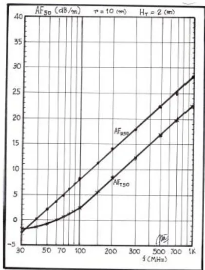
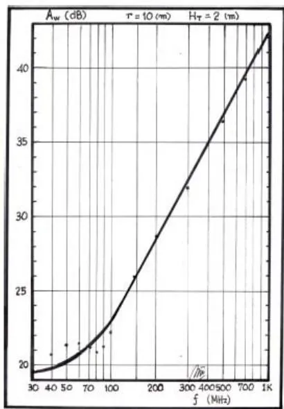
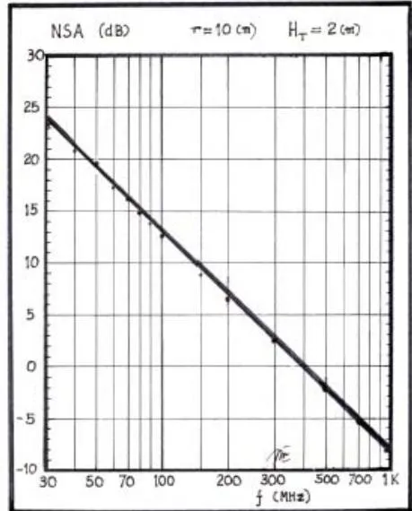
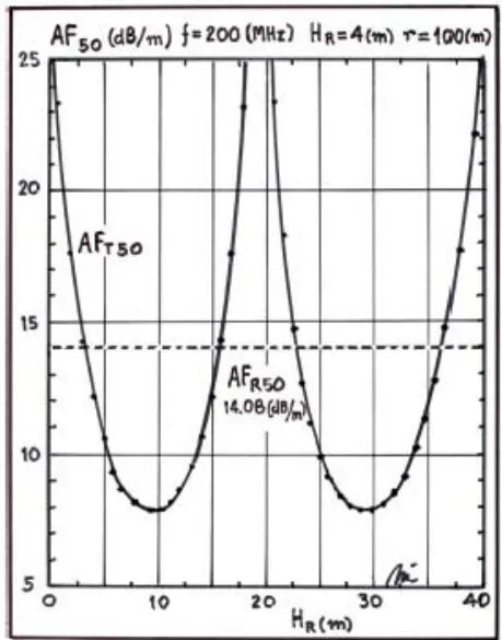
Calculation of several frequencies for the radio link of and r = 10[m] along the spectrum from 30 to 1000 MHz are presented in Figure 2, Figure 3 and Figure 4.
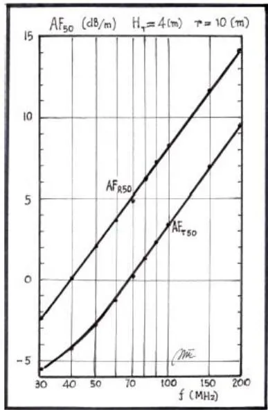
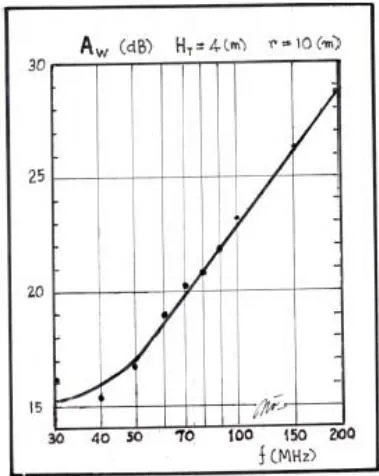
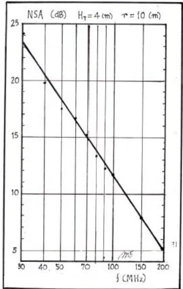
The transmission loss or site attenuation results are located on a straight line as plotted for the logarithmic frequency. A deviation is shown in the lower part of the spectrum where the transmitting antenna (Tx) height ( ) do not permit to get its maximum radiation between antennas in the radio link. This effect can be avoided increasing the Tx antenna height. At the same time, the perfect far field is really not achieved and for this reason the Rx antenna gain is not exactly 2.15 dBi. However, the conditions of far field are quite close if the maximum radiation is fulfilled. The wave impedance are presented in the table II permitting to know its value. Perfect far field corresponds when the wave impedance is exactly the space intrinsic impedance or . The plot of the antenna factors have a difference close to 6 dB when the Tx antenna can develop the maximum radiation. The normalized site attenuation (NSA) is also located on a straight line as plotted for the logarithmic frequency. This is very important to take it into account.
| f(MHz) | (m) | (dBi) | (dBi) | (dB/m) | (dB/m) | |
| 30 | 6.00 | 2.05 | 0.63 | -2.40 | -1.96 | 12.77 |
| 50 | 6.00 | 2.16 | 6.00 | 2.04 | -0.99 | 4.71 |
| 70 | 6.00 | 2.18 | 6.70 | 4.96 | 0.07 | 2.41 |
| 100 | 5.72 | 2.19 | 7.69 | 8.06 | 2.27 | 1.19 |
| 200 | 2.84 | 2.19 | 8.25 | 14.08 | 8.31 | 0.30 |
| 300 | 1.86 | 2.19 | 7.86 | 17.60 | 12.00 | 0.13 |
| 500 | 1.13 | 2.19 | 8.12 | 22.04 | 16.23 | 0.05 |
| 700 | 0.79 | 2.19 | 7.95 | 24.96 | 19.21 | 0.02 |
| 1000 | 0.58 | 2.19 | 8.00 | 28.06 | 22.19 | 0.01 |
If the radio link distance r between antennas is increased it is important to determine its results because as distance is increased the Tx antenna elevation angle decreases and the far field conditions are obtained at a larger distance. Here a calculation can be seen for the Tx antenna height [m] and r=30 [m]. The receiving antenna (Rx) is scanned between [m] and [m]. These results are presented in table III and table IV. Only some frequencies are presented in these tables.
At the same time, all the results for several frequencies in the radio link of and along the spectrum from 30 to 1000 MHz are presented in Figure 5, Figure 6 and Figure 7. Here, also, the site attenuation must be on a straight line but at lower frequencies it has a deviation if the Tx antenna height is not at the proper height . This effect is avoided if the Tx antenna is at larger heights as shown here in Figure 6.
An additional calculation is performed for a radio link with a distance r = 10 [m] and an increase of the Tx antenna height to [m]. This permits to observe if an improvement on its results could be obtained at the lower frequencies.
| NSA | ||||||
| (MHz) | (dB) | (dB) | (Ω) | (dB) | ||
| 30 | 9.19 | 29.02 | 31.70 | 368.0 | 33.38 | -14.42 |
| 50 | 11.40 | 27.98 | 36.13 | 376.7 | 26.93 | -8.94 |
| 70 | 6.84 | 30.17 | 39.06 | 378.8 | 25.14 | -8.22 |
| 100 | 4.20 | 32.26 | 42.14 | 379.7 | 21.93 | -7.21 |
| 200 | 1.20 | 37.60 | 48.04 | 386.3 | 15.21 | -6.53 |
| 300 | 0.49 | 41.49 | 51.54 | 380.1 | 11.89 | -6.89 |
| 500 | 0.10 | 45.65 | 55.97 | 380.1 | 7.38 | -6.62 |
| 700 | 0.09 | 48.75 | 58.89 | 380.1 | 4.58 | -6.79 |
| 1000 | 0.04 | 51.79 | 61.99 | 380.0 | 1.64 | -6.73 |
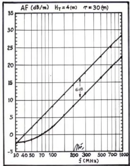
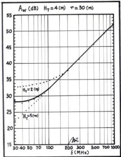
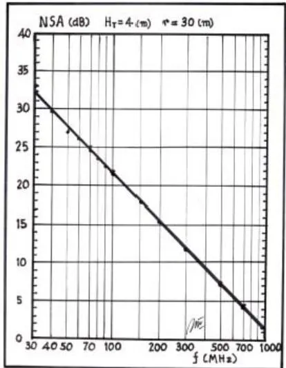
| (MHz) | (m) | (dBi) | (dBi) | (dB/m) | (dB/m) | |
| 30 | 4.00 | 2.11 | 4.30 | -2.40 | -5.58 | 12.93 |
| 40 | 4.00 | 2.29 | 7.45 | 0.10 | -4.40 | 7.59 |
| 50 | 4.00 | 2.36 | 8.14 | 2.04 | -2.92 | 4.93 |
| 60 | 3.30 | 2.39 | 6.92 | 3.62 | -1.25 | 3.45 |
| 70 | 2.77 | 2.42 | 6.94 | 4.96 | 0.10 | 2.55 |
| 80 | 2.40 | 2.43 | 7.70 | 6.12 | 1.35 | 1.96 |
| 90 | 2.13 | 2.44 | 7.48 | 7.15 | 2.48 | 1.55 |
| 100 | 1.91 | 2.45 | 6.86 | 8.06 | 3.37 | 1.26 |
| 150 | 1.26 | 2.46 | 7.20 | 11.58 | 6.91 | 0.56 |
| 200 | 0.95 | 2.47 | 7.36 | 14.08 | 9.46 | 0.32 |
These results are presented in table V and table VI. Only some frequencies are presented in these tables.
According to calculations the results are giving interesting results.
Rx antenna factors are obtained with exactly the same values as in the radio link with Tx antenna at the [m]. More constant site attenuation values in the lowest frequencies between 30 MHz and 70 MHz are seen. The site attenuation values are practically on a straight line with [m] but it could be even better if its height is [m]. No difference occurs for the Rx antenna factors because they are independent from the Tx antenna heights and distances.
All results for several frequencies in the radio link of and along the spectrum from 30 to 200 MHz are presented in Figure 8, Figure 9 and Figure 10.
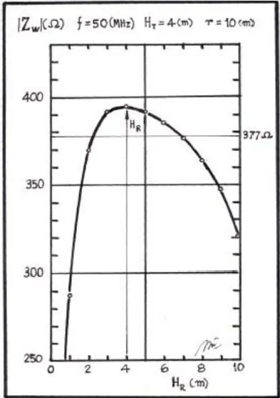
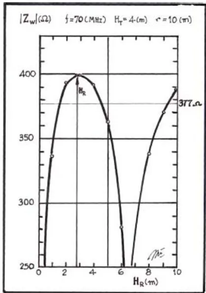
Far field do not only depends on distance r like in free space. Over a ground plane a radio link has a far field strongly dependent of the radiating elevation angle from the Tx antenna. For this reason in Figure 11, Figure 12 and Figure 13 the radio link wave impedance is plotted as a function of the Rx antenna height for the frequencies of 30, 50 and 70 MHz where and r = 10[m].
| f(MHz) | ( ) | (dB) | (dB) | (Ω) | NSA(dB) | (dBV/m) |
| 30 | 21.41 | 16.22 | 22.63 | 372.6 | 24.20 | -1.62 |
| 40 | 24.84 | 15.39 | 25.13 | 388.7 | 19.69 | 1.71 |
| 50 | 18.65 | 16.57 | 27.07 | 394.8 | 17.45 | 2.46 |
| 60 | 9.79 | 19.14 | 28.45 | 397.8 | 16.77 | 1.47 |
| 70 | 7.22 | 20.31 | 29.67 | 399.9 | 15.25 | 1.64 |
| 80 | 6.60 | 20.61 | 30.74 | 401.0 | 13.14 | 2.51 |
| 90 | 4.94 | 21.80 | 31.72 | 402.0 | 12.17 | 2.34 |
| 100 | 3.47 | 23.29 | 32.60 | 402.8 | 11.86 | 1.76 |
| 150 | 1.67 | 26.37 | 36.03 | 404.2 | 7.88 | 2.21 |
| 200 | 0.97 | 28.68 | 38.51 | 404.9 | 5.14 | 2.40 |
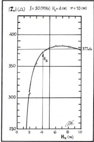
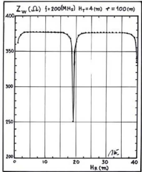
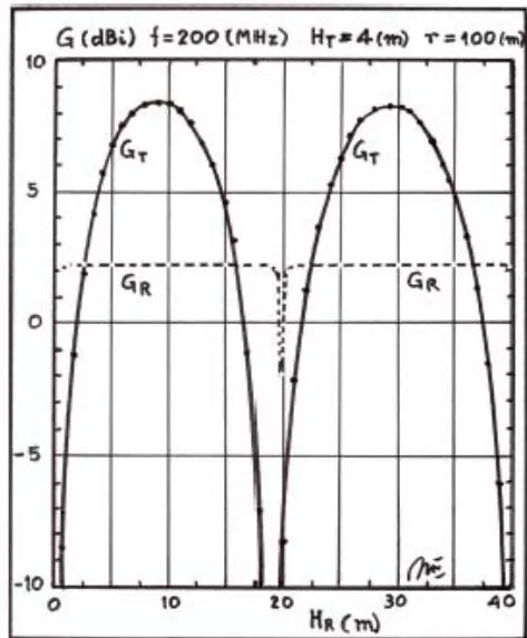
Wave impedance at short distances when real far field is not reached have large variation in its value as shown in several figures. This value is following the Tx antenna radiating lobes. Of course, increasing the distance r between antennas the wave antenna is reaching the far field value for any elevation angle .
Nevertheless, a calculation for and ( ) shows a sharp wave impedance
III. MEASUREMENT
Measurement needs an antenna range in order to verify the antenna parameters. To determine antenna gains the antenna range needs a proper site to fulfill the far field distance. This task is difficult to achieve at the lower frequencies between 30 and 100 MHz because the wave impedance must achieve a value very close or exactly . It was determined here that this value depends not only of the distance r but also by the elevation angle of the Tx radiation pattern.
This task was practically achieved very closely with an anechoic chamber of INTI, Buenos Aires, Argentina.
This chamber was used in order to verify the antenna factor of a Rohde und Schwarz precision half-wave dipole antennas model HZ-12 . The useful range of these antennas is between 30 and 300 MHz and recommended for horizontal polarization .
Horizontal polarization at the frequency of , was performed for this task. Taking into account the coaxial transmission and receiving lines as well the balun with matching system losses the radio link was deployed with a distance of and the Tx antenna was located at a fixed height of . Rx antenna had the possibility to be scanned between 1 and 4 [m]. Transmitted and received power were obtained by a Rohde und Schwarz generator and a Rohde und Schwarz spectrun analyzer. Transmitted power was adopted as 0 dBW and the received power was obtained as . Maximum power density or electric field was obtained at the Rx antenna height and the elevation angle from the Tx antenna center phase and the center of the Rx antenna is close to . With this angle the distance between the Tx center phase and the Rx center is so the free space loss results .
Loss relation:
On the equivalent Thevenin Rx antenna circuit the current results in:
Rx antenna load voltage results in:
Induced Voltage on the Rx antenna results in:
Rx antenna effective length:
Incoming electric field results in:
Incoming power density results in:
Rx antenna effective area results in:
Rx antenna numerical gain :
Rx antenna gain
Friis equation permits to know the true Tx antenna gain , thus:
Tx antenna numerical gain .
Checking the Tx antenna gain at the distance :
Tx antenna gain was calculated correctly.
Rx antenna factor results in:
Rx antenna factor
Rx antenna factor
Tx antenna factor results in:
Tx antenna factor Tx antenna factor
Normalized Site Attenuation (NSA) results in:
Using the Equation (7) of Standard C 63-5-2004:
With equation (7) the result is the same as Rx antenna factor previously obtained.
Using the FCC Equation obtained from and far field condition, results in:
These values are equal to that obtained previously by calculation.
Applying the Friis equation in dB over perfect ground (metallic ), the result is:
It can be seen here that the Friis Power Budget is perfectly fulfilled.
Tx antenna effective area :
Applying the Schelkunoff and Friis Power Reciprocity Principle:
| S | M | S | M | S | M | |
| (m) | (V/m) | (V/m) | (dBi) | (dBi) | ||
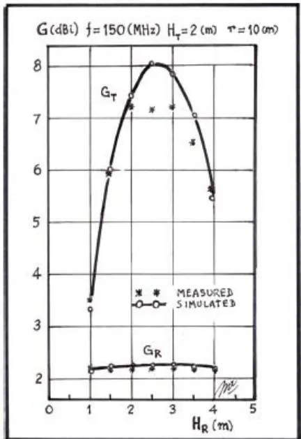
| 1.0 | 0.795 | 0.817 | 1.71E-3 | 1.77E-3 | 3.37 | 3.52 |
| 1.5 | 1.089 | 1.080 | 3.13E-3 | 3.10E-3 | 6.04 | 6.00 |
| 2.0 | 1.276 | 1.230 | 4.26E-3 | 4.01E-3 | 7.46 | 7.20 |
| 2.5 | 1.348 | 1.190 | 4.74E-3 | 3.76E-3 | 8.02 | 7.02 |
| 3.0 | 1.309 | 1.190 | 4.48E-3 | 3.76E-3 | 7.88 | 7.12 |
| 3.5 | 1.176 | 1.090 | 3.63E-3 | 3.15E-3 | 7.09 | 6.48 |
| 4.0 | 0.973 | 0.983 | 2.51E-3 | 2.56E-3 | 5.63 | 5.72 |
Table 8: Comparison between Simulated (S) and Measurement (M),
[M] and r = 10 [M], F = 150 (MHZ)
| S | M | S | M | S | M | |
| (m) | (dBi) | (dBi) | ( ) | (dB) | (dB) | |
| 1.0 | 2.08 | 2.16 | 0.51 | 0.52 | 30.56 | 30.33 |
| 1.5 | 2.20 | 2.15 | 0.53 | 0.52 | 27.83 | 27.90 |
| 2.0 | 2.22 | 2.14 | 0.53 | 0.52 | 26.47 | 26.80 |
| 2.5 | 2.22 | 2.14 | 0.53 | 0.52 | 25.98 | 27.07 |
| 3.0 | 2.22 | 2.18 | 0.53 | 0.53 | 26.23 | 27.04 |
| 3.5 | 2.20 | 2.16 | 0.53 | 0.52 | 27.16 | 27.83 |
| 4.0 | 2.15 | 2.16 | 0.53 | 0.52 | 28.82 | 28.74 |
The Power Reciprocity Principle is also fulfilled. For this measurement it was supposed that the wave impedance or at the real far field. Calculation with the same radio link geometry are giving a wave impedance . This value is very close to the real far field for the radiation maximum of the Tx antenna at the elevation angle , and its result error is negligible. Other possible difference could be using the radiation resistance of both antenna as . In this case if the mismatch is lower than 1.5 in VSWR the mismatching losses could produce an error lower than 0.2 dB.
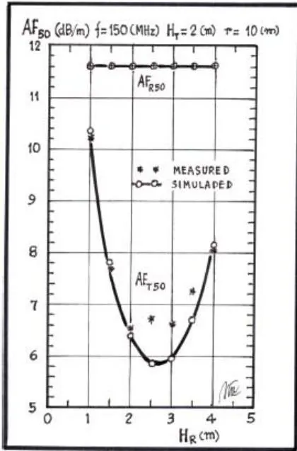
In order to make the task more complete measurements were performed at several Rx antenna heights and simulated at the same Rx heights. These results are compared in table VII, table VIII and table IX. Results are also presented in Figure 17 and Figure 18.
| S | M | S | M | S | M | |
| (m) | (dB/m) | (dB/m) | (dB/m) | (dB/m) | (W) | (W) |
| 1.0 | 11.58 | 11.58 | 10.35 | 10.22 | 30.56 | 30.33 |
| 1.5 | 11.57 | 11.58 | 7.79 | 7.74 | 27.83 | 27.90 |
| 2.0 | 11.59 | 11.58 | 6.40 | 6.54 | 26.47 | 26.80 |
| 2.5 | 11.58 | 11.59 | 5.85 | 6.73 | 25.98 | 27.07 |
| 3.0 | 11.58 | 11.60 | 5.98 | 6.63 | 26.23 | 27.04 |
| 3.5 | 11.59 | 11.56 | 6.74 | 7.27 | 27.16 | 27.83 |
| 4.0 | 11.60 | 11.58 | 8.18 | 8.01 | 28.82 | 28.74 |
IV. CONCLUSIONS
In conclusion it was found to be correct the power gain and antenna factor from Rohde und Schwarz model HZ-12 antenna manual [19]. Rx antenna factor as well its effective length are parameters not depending on the far field of the electromagnetic waves. It was determined that the effective length depends from the current distribution on its physical structure but if the current distribution is unknown it can be determined by the relation between the induced voltage at open circuit on the Rx antenna and the incoming electric field [14].
Simulation and measurements are confirming this statement. This relation is valid in near and far field and it produces always the same results. Rx antenna factor is also independent of its height over ground and distance because it operates practically like in free space. For this reason a half-wave dipole antenna can be adopted as a natural standard sensor useful to calibrate any other antenna at any frequency between 30 and 1000 MHz [11]. On the contrary, the Tx antenna factor is not constant and depends on its gain over perfect ground considering it is an array of two elements [2],[3],[6], the actual antenna and its image. Of course its factor is different as well the gain from that of the Rx antenna as was shown in this paper results [8].
Rx antenna gain and effective area are far field parameters and they acquire the proper value when the wave impedance is . In this paper it was clearly obtained the Rx antenna factor with exactly the same value in any radio link for several distance r and for any Tx antenna height using the relation . Main Friis equation is useful and valid over perfect ground [1], as was perfectly demostated and it gives a perfect power budget between losses ( ) and gains ( ). No additional factors are needed, as was published [12], [21], but only the true gains ( ) as was determined here. Also with these results, the reciprocity power principle ( ) is fulfilled according to Schelkunoff and Friis [3]. The transmitting antenna is a simple devise and it only needs to radiate the EM energy in the surrounding space. Receiving antenna is a more complex device because it needs to operate in two roles, the receiving role and the retransmitting or scattering role. For this reason, in a radio link with two identical half wave dipole antennas in horizontal polarization, the theoretical transmitting antenna gain is , the receiving antenna gain is and the scattering gain is . The effective receiving area is the relation between the power received and the incoming power density . The scattering effective area , according to Friis, is the product between the isotropic source area and the scattering numerical gain . The gain difference between the transmitting antenna gain and the receiving antenna gain is really 6 dB, according to calculations and measurements.
ACKNOWLEDGMENTS
I would like to express my appreciation to Ramiro Alonso, Walter Gustavo Fano and Lucas Gonzalez for the written version and computational support. Also support from INTI personnel Edmundo Gatti, Luciano Blas and Matias Fernandez is very much appreciated.