## I. INTRODUCTION $$ D _ {t} = f \left(\mathbf {X} _ {t}; \boldsymbol {\theta}\right) + \varepsilon_ {t} $$ $$ \min_{Q_t s_t} \mathbb{E}\left[\sum_t \left(h \cdot I_t^+ + b \cdot I_t^- + k \cdot \delta(Q_t)\right)\right] $$ $$ I _ {t} = I _ {t - 1} + Q _ {t} - D _ {t} $$ Inventory optimization remains a cornerstone of supply chain management, with the Economic Order Quantity (EOQ) model serving as its bedrock for over a century [1]. Yet, traditional EOQ frameworks—reliant on static assumptions of demand, costs, and lead times—increasingly fail in today's volatile markets characterized by disruptions, demand spikes, and perishability constraints [2]. While stochastic EOQ variants [3] and dynamic programming approaches [4] address known uncertainties, they lack adaptability to real-time data and struggle with high-dimensional, nonstationary variables [5]. Recent advances in Artificial Intelligence (AI) offer transformative potential. Machine learning (ML) enables granular demand sensing by synthesizing covariates like promotions, social trends, and macroeconomic indicators [6], while reinforcement learning (RL) autonomously optimizes decisions under uncertainty [7]. However, extant studies focus narrowly on either forecasting [8] or policy optimization [9] in isolation, neglecting closed-loop, dynamic control that unifies both. This gap is acute in sector-specific contexts: - Perishable goods (e.g., pharmaceuticals) suffer from expiry losses under fixed-order policies [10], - Promotion-driven retail faces costly stockouts during demand surges [11], - Multi-echelon manufacturing battles component shortages due to rigid reorder points [12]. This research bridges these gaps by proposing an integrated AI-ML framework for dynamic EOQ control. Our contributions are: 1. A dynamic inventory system formalized via time-dependent equations: - Demand: $D_{t} = f(\mathbf{X}_{t};\theta) + \epsilon_{t}$ (ML-estimated) [13], - Cost minimization: $\min_{Q_t,s_t}\mathbb{E}[\sum_t(h\cdot I_t^+ +b\cdot I_t^- +k\cdot \delta (Q_t))]$ (RL-optimized) [7], subject to $I_{t} = I_{t - 1} + Q_{t} - D_{t}$ ### 2. Sector-specific innovations: - Perishability constraints $(I_t^+ \leq \tau)$ for pharmaceuticals [10], - Promotion-responsive safety stocks $(s_{t} = \mu_{t} + z\cdot \sigma_{t})$ for retail [11], - Multi-echelon RL agents for automotive supply chains [12]. 3. Empirical validation across three industries demonstrating $>24\%$ cost reduction versus state-of-the-art benchmarks [3,5,9]. ## II. RESEARCH METHODOLOGY This study employs a hybrid AI-operations research framework to develop dynamic EOQ policies. The methodology comprises four phases, validated across pharmaceutical, retail, and automotive sectors. ### a) Dynamic EOQ Problem Formulation The inventory system is modeled as a Markov Decision Process (MDP) with: - State space: $\mathcal{S}_t = (I_t, D_{t-1:t-k}, \mathbf{X}_t)$ (Inventory $I_t$, lagged demand $D$, covariates $\mathbf{X}_t$: promotions, lead times, seasonality) - Action space: $\mathcal{A}_t = (Q_t, s_t)$ (Order quantity $Q_t$, reorder point $s_t$ ) - $Cost\ function: C_t = \underbrace{h \cdot I_t^+}_{\text{Holding}} + \underbrace{b \cdot \max(-I_t, 0)}_{\text{Backordering}} + \underbrace{k \cdot \delta(Q_t)}_{\text{Ordering}} + \underbrace{\lambda \cdot \mathbb{1}_{I_t^+ > \tau}}_{\text{Perishability penalty}}$ - Objective: Minimize $\mathbb{E}[\sum_{t=0}^{T} \gamma^t C_t]$ ( $\gamma$: discount factor; $T$: horizon) ### b) Phase 1: Demand Forecasting (ML Module) Algorithms: - LSTM Networks: For pharma (perishable demand with expiry constraints) $\hat{D}_t = \mathrm{LSTM}(\mathbf{X}_t^{\mathrm{(pharma)}}; \theta_{\mathrm{LSTM}})$ where $\mathbf{X}_t = [\text{seasonality, disease rates, shelf-life}]$ - Gradient Boosted Regression Trees (GBRT): For retail (promotion-driven spikes) - Training: - Data: 24 months of historical sales + exogenous variables (Table 1) - Hyperparameter tuning: Bayesian optimization (Tree-structured Parzen Estimator) - Validation: Time-series cross-validation (MAPE, RMSE) Table 1: Sector-Specific Datasets <table><tr><td>Sector</td><td>Data Features</td><td>Size</td></tr><tr><td>Pharmaceuticals</td><td>Historical sales, disease incidence, expiry rates</td><td>500K SKU-months</td></tr><tr><td>Retail</td><td>POS data, promo calendars, social trends</td><td>1.2M transactions</td></tr><tr><td>Automotive</td><td>Component lead times, BOM schedules</td><td>320K part records</td></tr></table> ### c) Phase 2: Dynamic Policy Optimization (RL Module) Algorithm: Proximal Policy Optimization (PPO) with actor-critic architecture - Actor: Policy $\pi_{\phi}(Q_t|\mathcal{S}_t)$ - Critic: Value function $V_{\psi}(\mathcal{S}_t)$ - Reward design: $r_t = -(C_t - C_{\mathrm{benchmark}})$ (Benchmark: Classical EOQ cost) - Training: - Environment: Simulated supply chain (Python + OpenAI Gym) - Exploration: Gaussian noise $\mathcal{N}(0,\sigma_t)$ for $Q_{t}$ - Termination: Policy convergence ( $\Delta C_t < 0.1\%$ for $10\mathrm{k}$ steps) ### d) Phase 3: Sector-Specific Adaptations #### 1. Pharma: - Constraint: $I_t^+ \leq \tau$ (shelf-life) - Penalty: $\lambda = 2b$ (expired unit cost $= 2\times$ backorder cost) #### 2. Retail: - Safety stock: $s_t = \mu_t + z \cdot \sigma_t$ with $z$ tuned by RL. #### 3. Automotive: - Multi-echelon state: $\mathcal{S}_t^{(\mathrm{auto})} = (I_t^{\mathrm{warehouse}}, I_t^{\mathrm{assembly}}, \mathrm{lead~time}_t)$ ### e) Phase 4: Validation & Benchmarking - Baselines: - Classical EOQ: $Q^{*} = \sqrt{\frac{2kD}{h}}$ - (s,S) Policy (Scarf, 1960) - Stochastic EOQ (Zipkin, 2000) - Metrics: - Total cost reduction: $\frac{C_{\mathrm{baseline}} - C_{\mathrm{AI-EOQ}}}{C_{\mathrm{baseline}}} \times 100\%$ - Service level: $\mathrm{SL} = 1 - \frac{\mathrm{stockout~instances}}{\mathrm{total~periods}}$ - Hardware: NVIDIA V100 GPUs, 128 GB RAM - Software: Python 3.9, Tensor Flow 2.8, OR-Tools ## III. MATHEMATICAL FORMULATION: AI-DRIVEN DYNAMIC EOQ MODEL Core Components: 1. Time-Varying Demand Forecasting 2. Reinforcement Learning Optimization 3. Sector-Specific Constraints ### a) Demand Dynamics Let demand $D_{t}$ be modeled as: $$ D _ {t} = f (\mathbf {X} _ {t}; \boldsymbol {\theta}) + \epsilon_ {t} $$ - $X_{t}$: Feature vector (promotions, seasonality, market indicators) - $\theta$: Parameters of ML model (LSTM/GBRT) - $\epsilon_{t} \sim \mathcal{N}(0, \sigma_{t}^{2})$: Residual with time-dependent volatility LSTM Formulation: $$ i_{t} = \sigma(W_{i} \cdot [\mathbf{h}_{t-1}, \mathbf{X}_{t}] + b_{i}) $$ $$ \mathbf{f}_{t} = \sigma(W_{f} \cdot [\mathbf{h}_{t-1}, \mathbf{X}_{t}] + b_{f}) $$ $$ \mathbf{o}_{t} = \sigma(W_{o} \cdot [\mathbf{h}_{t-1}, \mathbf{X}_{t}] + b_{o}) $$ $$ \tilde {\mathbf {c}} _ {t} = \tanh \left(W _ {c} \cdot [ \mathbf {h} _ {t - 1}, \mathbf {X} _ {t} ] + b _ {c}\right) $$ $$ \mathbf{c}_{t} = \mathbf{f}_{t} \odot \mathbf{c}_{t - 1} + \mathbf{i}_{t} \odot \tilde{\mathbf{c}}_{t} $$ $$ \mathbf{h}_{t} = \mathbf{o}_{t} \odot \operatorname{tanh}(\mathbf{c}_{t}) $$ $$ \hat{D}_{t} = W_{d} \cdot \mathbf{h}_{t} + b_{d} $$ ### b) Inventory Balance & Cost Structure State Transition: $$ I _ {t} = I _ {t - 1} + Q _ {t - L} - D _ {t} $$ - $I_{t}$: Inventory at period $t$ - $Q_{t}$: Order quantity (decision variable) - $L$: Stochastic lead time $\sim \mathcal{U}[L_{\min}, L_{\max}]$ Total Cost Minimization: $$ \min _ {Q _ {t}, s _ {t}} \mathbb {E} \left[ \right. \sum_ {t = 0} ^ {T} \gamma^ {t} \underbrace {\left(\quad h \cdot I _ {t} ^ {+} + b \cdot I _ {t} ^ {-} + k \cdot \delta (Q _ {t}) \right.} _ {\mathrm {B a s e E O Q C o s t s}} + \underbrace \lambda \cdot \mathbb {1} _ {(I _ {t} ^ {+} > \tau)} + \phi \cdot (s _ {t} - \mu_ {t}) ^ {2}\left. \right)\left. \right] $$ where: - $I_{t}^{+} = \max (I_{t},0)$ (Holding cost) - $I_{t}^{-} = \max (-I_{t},0)$ (Backorder cost) - $\delta(Q_{t}) = \begin{cases} 1 & \text{if } Q_{t} > 0 \\ 0 & \text{otherwise} \end{cases}$ (Ordering cost trigger) - $\lambda$: Perishability penalty $(\tau = \mathrm{shelf - life})$ - $\phi \cdot (s_t - \mu_t)^2$: Safety stock deviation cost ( $\mu_t =$ forecasted mean) ### c) Reinforcement Learning Optimization MDP Formulation: - State: $\mathcal{S}_t = (I_t, \hat{D}_{t:t-H}, \mathrm{X}_t, Q_{t-1})$ ( $H = \text{lookback horizon}$ ) - Action: $\mathcal{A}_t = (Q_t, s_t)$ - Reward: $r_t = -(C_t - C_{\mathrm{benchmark}})$ PPO Policy Update: $$ \theta_{k+1} = \underset{\theta}{\arg\max}\mathbb{E}\left[\min\left(\frac{\pi_\theta(\mathcal{A}_t|\mathcal{S}_t)}{\pi_{\theta_k}(\mathcal{A}_t|\mathcal{S}_t)}A_t, \mathrm{clip}\left(\frac{\pi_\theta}{\pi_{\theta_k}}, 1-\epsilon, 1+\epsilon\right)A_t\right)\right] $$ $$ A_{t} = \sum_{i=0}^{T-t} (\gamma\lambda)^{i} \delta_{t+i}(\mathrm{GAE}) $$ $$ \delta_ {t} = r _ {t} + \gamma V _ {\psi} (\mathcal {S} _ {t + 1}) - V _ {\psi} (\mathcal {S} _ {t}) $$ where $\theta =$ actor params, $\psi =$ critic params, $\lambda =$ GAE parameter. ### d) Sector-Specific Constraints Pharmaceuticals (Perishability): $$ I _ {t} ^ {+} \leq \tau \Rightarrow Q _ {t} \leq \tau - I _ {t - 1} + D _ {t} $$ Retail (Promotion Safety Stock): $$ s _ {t} = \mu_ {t} + z \cdot \sigma_ {t}, z = g (\mathbf {X} _ {t} ^ {\mathrm {p r o m o}}; \theta_ {z}) $$ Automotive (Multi-Echelon Coordination): $$ \min_{Q_t^{(1)}, Q_t^{(2)}} \sum_{e=1}^2 \left(k^{(e)} \delta(Q_t^{(e)}) + h^{(e)} I_t^{(e)+}\right) \mathrm{s.t.} I_t^{(2)} = I_{t-1}^{(2)} + Q_{t-L_1}^{(1)} - Q_t^{(2)} $$ ### e) Performance Metrics 1. Cost Reduction: $\Delta C = \frac{C_{\mathrm{EOQ}} - C_{\mathrm{AI-EOQ}}}{C_{\mathrm{EOQ}}} \times 100\%$ 2. Service Level: $\mathrm{SL} = 1 - \frac{\sum_{\mathrm{t}}\mathrm{I}_{\mathrm{t}}^{-}}{\sum_{\mathrm{t}}\mathrm{D}_{\mathrm{t}}}$ 3. Waste Rate: $\xi = \frac{\sum_{\mathrm{t}} \max(\mathrm{I}_{\mathrm{t}}^{+} - \tau, 0)}{\sum_{\mathrm{t}} Q_{\mathrm{t}}}$ (Pharma) ## IV. MATHEMATICAL MODEL EQUATIONS: DEMAND FORECASTING ML MODULE Core Objective: Predict time-varying demand $D_{t}$ using covariates $\mathbf{X}_{t}$ Two Algorithms: LSTM (Pharma/Retail) and GBRT (Retail/Automotive) ### a) LSTM Network for Perishable Goods (Pharma) Input: Time-series features $\mathbf{X}_t = \left[\mathrm{sales}_{t-1:t-k}, \mathrm{disease}^{**}\mathrm{rate}_t, \mathrm{promos}_t, \mathrm{seasonality}_t\right]$ Equations: $$ Forget gate: f_{t} = \sigma(W_{f} \cdot [h_{t-1},\mathbf{F}X_{t}] + b_{f}) $$ $$ Input gate: i_{t} = \sigma(W_{i} \cdot [h_{t-1},\mathbf{X}_{t}] + b_{i}) $$ $$ Candidate state: \tilde{C}_{t} = \tanh \left( W_{C} \cdot [ h_{t-1},\mathbf{X}_{t} ] + b_{C} \right) $$ $$ \mathrm {C e l l s t a t e :} C _ {t} = f _ {t} \odot C _ {t - 1} + i _ {t} \odot \tilde {C} _ {t} $$ $$ Output~gate: o_{t} = \sigma(W_{o} \cdot [h_{t-1},\mathbf{X}_{t}] + b_{ ext{o}}) $$ $$ Hidden state: h_{t} = o_{t} \odot \tanh (\mathcal{C}_{t}) $$ $$ Demand forecast:\hat{D}_{t} = W_{d} \cdot h_{t} + b_{d} $$ Loss Function (Perishability-adjusted MSE): $$ \mathcal {L} _ {\mathrm {L S T M}} = \frac {1}{T} \sum_ {t = 1} ^ {T} \left(\underbrace {(D _ {t} - \hat {D} _ {t}) ^ {2}} _ {\mathrm {F o r e c a s t e r r o r}} + \lambda \cdot \underbrace {\max (I _ {t} ^ {+} - \tau , 0)} _ {\mathrm {E x p i r y p e n a l t y}}\right) $$ - $\sigma$: Sigmoid, $\odot$: Hadamard product - $\tau$: Shelf-life, $\lambda$: Perishability weight b) Gradient Boosted Regression Trees (GBRT) for Promotion-Driven Demand (Retail) Model: Additive ensemble of $M$ regression trees: $$ \hat{D}_{t} = \sum_{m=1}^{M} f_{m}(\mathbf{X}_{t}), f_{m} \in \mathcal{T} $$ Objective Function (Regularized): $$ \mathcal {L} _ {\mathrm {G B R T}} = \sum_ {t = 1} ^ {T} L (D _ {t}, \hat {D} _ {t}) + \sum_ {m = 1} ^ {M} \Omega (f _ {m}) \mathrm {w h e r e} \Omega (f) = \gamma T _ {\mathrm {l e a v e s}} + \frac {1}{2} \lambda \| \mathbf {w} \| ^ {2} $$ - L: Huber loss = $\begin{cases} \frac{1}{2} (D_t - \hat{D}_t)^2 & |D_t - \hat{D}_t| \leq \delta \\ \delta |D_t - \hat{D}_t| - \frac{1}{2}\delta^2 & \text{otherwise} \end{cases}$ - $w$: Leaf weights, $T_{\text{leaves}}$: Leaves per tree Tree Learning (Step $m$ ): 1. Compute pseudo-residuals: $r_t = -\frac{\partial L(D_t, \hat{D}_t^{(m-1)})}{\partial D_t^{(m-1)}}$ 2. Fit tree $f_{m}$ to $\{(\mathbf{X}_t,r_t)\}$ 3. Optimize leaf weights $w_{j}$ for leaf $j: w_{j}^{*} = \frac{\sum_{\mathbf{X}_{t} \in j} r_{t}}{\sum_{\mathbf{X}_{t} \in j} \frac{\partial^{2} L}{\partial (\hat{D}_{t})^{2}} + \lambda}$. ### c) Feature Engineering & Covariate Structure Input Feature Space: $$ \mathbf {X} _ {t} = \left[ \underbrace {D _ {t - 1} , D _ {t - 7} , D _ {t - 3 0}} _ {\mathrm {T e m p o r a l l a g s}}, \underbrace {\mathrm {p r o m o} “ \mathrm {i n t e n s i t y} _ {t}} _ {\mathrm {0 - 1 s c a l e}}, \underbrace {\Delta \mathrm {C P I} _ {t}} _ {\mathrm {E c o n o m i c i n d i c a t o r}}, \underbrace {\mathrm {t r e n d} “ \mathrm {s c o r e} _ {t}} _ {\mathrm {S e n t i m e n t a n a l y s i s}} \right] $$ Normalization: $$ \mathbf{X}_{t}^\mathrm{norm} = \frac{\mathbf{X}_{t} - \boldsymbol{\mu}_{\mathrm{train}}}{\boldsymbol{\sigma}_{\mathrm{train}}} $$ ### d) Uncertainty Quantification Demand Distribution Modeling: $$ D_{t} \sim \mathcal{N}(\mu_{t},\sigma_{t}^{2}) \text{where} \mu_{t} = \hat{D}_{t}, \sigma_{t} = g(\mathbf{X}_{t}) $$ Volatility Network (Auxiliary LSTM): $$ \sigma_ {t} = \mathrm {R e L U} \Big (W _ {\sigma} \cdot h _ {t} ^ {(\sigma)} + b _ {\sigma} \Big) $$ $$ h_{t}^{(\sigma)} = \mathrm{LSTM}( |D_{t-1} - \hat{D}_{t-1}|, \dots , |D_{t-k} - \hat{F}_{t-k}| ) $$ Table 2: Sector-Specific Adaptations <table><tr><td>Sector</td><td>ML Model</td><td>Special Features</td><td>Loss Adjustment</td></tr><tr><td>Pharma</td><td>LSTM</td><td>disease'rate, shelf'life'remaining</td><td>λ = 0.5 (High waste penalty)</td></tr><tr><td>Retail</td><td>GBRT + Volatility LSTM</td><td>promo'intensity, social'mentions</td><td>Huber loss (δ = 1.5)</td></tr><tr><td>Automotive</td><td>GBRT</td><td>supply'delay, BOM'volatility</td><td>γ = 0.1 (Tree complexity)</td></tr></table> ## V. MATHEMATICAL MODEL: DYNAMIC POLICY OPTIMIZATION (RL MODULE) Core Objective: Find adaptive policy $\pi^{*}(Q_{t},s_{t}\mid \mathcal{S}_{t})$ minimizing expected total cost a) Markov Decision Process (MDP) Formulation State Space: $$ \mathcal{S} _ {t} = \left(I _ {t}, \underbrace{\hat{D} _ {t} , \hat{D} _ {t - 1} , \dots , \hat{D} _ {t - k}} _ {\mathrm{D e m and f o r e c a s t s}}, \underbrace{\mathbf{X} _ {t}} _ {\mathrm{C o v a r i a t e s}}, \underbrace{Q _ {t - 1} , s _ {t - 1}} _ {\mathrm{L a s t a c t i o n s}}\right) $$ - $I_{t}$: Current inventory - $\hat{D}_{t - i}$: ML forecasts (LSTM/GBRT output) - $X_{t}$: Exogenous features (promotions, lead times, etc.) Action Space: $$ \mathcal{A}_{t} = (Q_{t}, s_{t}) \mathrm{where} Q_{t} \in \mathbb{R}^{+}, s_{t} \in \mathbb{R} $$ Transition Dynamics: $$ I _ {t + 1} = I _ {t} + Q _ {t} - D _ {t}, D _ {t} \sim \mathcal {N} (\hat {D} _ {t}, \sigma_ {t} ^ {2}) $$ $(\sigma_{t}$: Volatility from ML uncertainty quantification) ### b) Cost Function $$ C_{t} = h \cdot \max (I_{t}, 0) + b \cdot \max (- I_{t}, 0) + k \cdot \delta (Q_{t}) + \lambda \cdot \mathbb{1}_{[I_{t}^{+} > \tau]} + \phi \cdot (s_{t} - \mu_{t})^{2} $$ - $\delta (Q_{t}) = \left\{ \begin{array}{ll}1 & Q_{t} > 0\\ 0 & \mathrm{otherwise} \end{array} \right.$ - $\mu_t = \mathbb{E}[D_t]$: Forecasted mean demand #### Sector Penalties: - Pharma: $\lambda = 2b$ (high expiry cost) - Retail: $\phi = 0.1b$ (moderate safety stock flexibility) - Auto: $k_{\mathrm{multi - echelon}} = \sum_{e = 1}^{E}k^{(e)}\delta (Q_t^{(e)})$ ### c) Policy Optimization Objective $$ \max_{\pi} \mathbb{E}\left[\sum_{t=0}^{T} \gamma^{t} r_{t}\right] \mathrm{with} r_{t} = -C_{t} $$ $(\gamma \in [0,1]$: Discount factor ### d) Proximal Policy Optimization (PPO) Actor-Critic Architecture: - Actor: Policy $\pi_{\theta}(\mathcal{A}_t \mid S_t)$ - Critic: Value function $V_{\psi}(\mathcal{S}_t)$ Policy Update via Probability Ratio: $$ r _ {t} (\theta) = \frac {\pi_ {\theta} (\mathcal {A} _ {t} \mid \mathcal {S} _ {t})}{\pi_ {\theta_ {\mathrm {o l d}}} (\mathcal {A} _ {t} \mid \mathcal {S} _ {t})} $$ Clipped Surrogate Objective: $$ L ^ {\mathrm{C L I P}} (\theta) = \mathbb{E} _ {t} \big [ \min (r _ {t} (\theta) A _ {t}, \operatorname{clip} (r _ {t} (\theta), 1 - \epsilon , 1 + \epsilon) A _ {t}) \big ] $$ - $\epsilon = 0.2$: Clip range - $A_{t}$: Advantage estimate (GAE) Generalized Advantage Estimation (GAE): $$ A _ {t} = \sum_ {l = 0} ^ {T - t} (\gamma \lambda_ {\mathrm {G A E}}) ^ {l} \delta_ {t + l} $$ $$ \delta_{t} = r_{t} + \gamma V_{\psi}(\mathcal{S}_{t+1}) - V_{\psi}(\mathcal{S}_{t}) $$ $$ (\lambda_{GAE} = 0.95) $$ Critic Loss (Mean-Squared Error): $$ L(\psi) = \mathbb{E}_{t} \left[ (V_{\psi}(\mathcal{S}_{t}) - \hat{V}_{t})^{2} \right], \hat{V}_{t} = \sum_{l=0}^{T-t} \gamma^{l} r_{t+l} $$ ### e) Action Distribution Gaussian Policy with State-Dependent Variance: $$ Q _ {t} \sim \mathcal {N} \big (\mu_ {Q} (\mathcal {S} _ {t}), \sigma_ {Q} ^ {2} (\mathcal {S} _ {t}) \big), s _ {t} \sim \mathcal {N} (\mu_ {s} (\mathcal {S} _ {t}), \sigma_ {s} ^ {2} (\mathcal {S} _ {t})) $$ Neural Network Output: $$ \left[ \begin{array}{c} \mu_ {Q} \\\mu_ {s} \\\log \sigma_ {Q} \\\log \sigma_ {s} \end{array} \right] = \mathrm{MLP}_\theta (\mathcal{S}_t) $$ ### f) Sector-Specific Constraints (Hardcoded in Environment) 1. Pharma: $Q_{t} \leq \max(0, \tau - I_{t}^{+} + \hat{D}_{t})$ 2. Retail: $s_t \in [\mu_t - 3\sigma_t, \mu_t + 3\sigma_t]$ 3. Auto(Multi-Echelon): $Q_{t}^{(e)} \leq I_{t}^{(e-1)} \text{ for } e = 2, \ldots, E$ Training Protocol #### 1. Simulation Environment: - Lead times: $L \sim \operatorname{Weibull}(k = 1.5, \lambda = 7)$ - Demand shocks: $D_{t} = \hat{D}_{t}\cdot (1 + \eta_{t}),\eta_{t}\sim \mathcal{N}(0,0.2^{2})$ #### 2. Hyperparameters: - Optimizer: Adam $(\alpha_{\mathrm{actor}} = 10^{-4}, \alpha_{\mathrm{critic}} = 3 \times 10^{-4})$ - Batch size: 64 episodes $\times$ 30 time steps - Discount: $\gamma = 0.99$ 3. Termination: $\| \nabla_{\theta}L^{\mathrm{CLIP}}\| _2 < 0.001$ and $\frac{|C_t - C_{t - 1000}|}{C_t} < 0.005$ ## VI. MATHEMATICAL MODEL: SECTOR-SPECIFIC ADAPTATIONS CORE EQUATIONS FOR PHARMA, RETAIL, AND AUTOMOTIVE SECTORS ### a) Pharmaceuticals (Perishable Goods) ## i. Constrained State Space $$ \mathcal{S} _ {t} ^ {\mathrm{(p h a r m a)}} = \left(I _ {t} ^ {+}, \underbrace{\tau - t _ {\mathrm{e l a p s e d}}} _ {\mathrm{R e m a i n i n g s h e l f - l if e}}, \hat{D} _ {t}, \mathrm{d i s e a s e} ^ {\prime \prime} \mathrm{r a t e} _ {t}\right) $$ - $t_{\text{ elapsed}}$: Time since production ## ii. Perishability-Constrained Actions $$ Q_{t} = \left\{ \begin{array}{l l} \max \big (0, \tau \cdot \hat{D}_{t} - I_{t}^{+} \big) & \text{if } t_{\mathrm{elapsed}} \geq 0.7 \tau \\ \pi_{\theta} \left(\mathcal{S}_{t}\right) & \text{otherwise} \end{array} \right. $$ ## iii. Modified Cost Function - $\lambda = 3b$ (base penalty), $\kappa$: Decay rate - Justification: Penalizes inventory approaching expiry (Bakker et al. 2012) ### b) Retail (Promotion-Driven Volatility) i. Augmented State Space: ii. Dynamic Safety Stock Policy: $$ s_{t} = \mathrm{softplus}(\mu_{t} + z_{t} \cdot \sigma_{t})\,\mathrm{where}\,z_{t} = \mathrm{MLP}_{\phi}(\mathrm{promo}“\mathrm{intensity}_{t},\mathrm{sentiment}_{t}) $$ ## iii. Promotion-Aware Cost Adjustment $$ C _ {t} ^ {\mathrm {(r e t a i l)}} = \underbrace {C _ {t}} _ {\mathrm {B a s e}} + \underbrace {\beta \cdot \left| \sigma_ {t} ^ {\mathrm {(a c t u a l)}} - \sigma_ {t} ^ {\mathrm {(M L)}} \right|} _ {\mathrm {V o l a t i l i t y m i s m a t c h p e n a l t y}} $$ - $\beta = 0.5h,\sigma_t^{(\mathrm{actual})} = \mathrm{std}(D_{t - 7:t})$ - Justification: Adaptive safety stock during promotions (Trapero et al. 2019) ### c) Automotive (Multi-Echelon Supply Chain) ## i. Hierarchical State Space $$ \mathcal{S}_{t}^{(\mathrm{auto})} = \left(\underbrace{I_{t}^{(1)}, I_{t}^{(2)}}_{\mathrm{Echelon~inventories}}, \underbrace{Q_{t}^{(1)}, Q_{t}^{(2)}}_{\mathrm{Pending~orders}}, \underbrace{\mathbf{L}_{t}}_{\mathrm{Lead~time~vector}}\right) $$ $\mathrm{L}_t = [L_t^{(\mathrm{supplier~1})}, L_t^{(\mathrm{supplier~2})}]$ ## ii. Coordinated Order Policy $$ \left[ \begin{array}{c} Q _ {t} ^ {(1)} \\Q _ {t} ^ {(2)} \end{array} \right] = \pi_ {\theta} (\mathcal {S} _ {t}) + \epsilon_ {t} \mathrm {s . t .} \epsilon_ {t} \sim \mathcal {N} (0, \Sigma_ {t}) $$ $$ \Sigma_ {t} = \left( \begin{array}{c c} \sigma_ {t} ^ {(1)} & \rho \sigma_ {t} ^ {(1)} \sigma_ {t} ^ {(2)} \\\rho \sigma_ {t} ^ {(1)} \sigma_ {t} ^ {(2)} & \sigma_ {t} ^ {(2)} \end{array} \right), \rho = -0.8 $$ (Negatively correlated exploration) ## iii. Echelon-Coupled Cost Function $$ C _ {t} ^ {\mathrm{(a u t o)}} = \sum_ {e = 1} ^ {2} \left(h ^ {(e)} I _ {t} ^ {(e) +} + b ^ {(e)} I _ {t} ^ {(e) -}\right) + \eta \cdot \underbrace{\left| I _ {t} ^ {(1)} - \alpha I _ {t} ^ {(2)} \right|}_{\mathrm{I m b a l i n c e p e n a l t y}} $$ - $\eta = 0.3h^{(1)}$, $\alpha = 0.6$ (ideal echelon ratio) - Justification: Penalizes inventory imbalances (Govindan et al. 2020) ## VII. SECTOR-SPECIFIC TRANSITION DYNAMICS ### a) Pharma: Perishable Inventory Update $$ I _ {t + 1} ^ {+} = \max \left(0, I _ {t} ^ {+} + Q _ {t} - D _ {t} - \left\lfloor \frac {I _ {t} ^ {+}}{\tau} \right\rfloor \cdot I _ {t} ^ {+}\right) $$ - Floor term models expired stock removal ### b) Retail: Promotion-Driven Demand Shock $$ D_{t}^{(retail)} = \hat{D}_{t} \cdot \left(1 + \mathrm{promo"intensity}_{t} \cdot \Delta_{max}\right) + \sigma_{t} \cdot \xi_{t}, \xi_{t} \sim \mathrm{Gumbel}(0, 1) $$ $\Delta_{\mathrm{max}} = 2.0$ (max demand uplift) ### c) Automotive: Lead Time-Dependent Receipts $$ I_{t+L^{(e)}}^{(e)} \gets I_{t+L^{(e)}}^{(e)} + Q_t^{(e)} \mathrm{\,where\,} L^{(e)} \sim \mathrm{\gamma}(k_e,\theta_e) $$ - \gamma distribution models component-specific delays Table 3: Mathematical Innovations <table><tr><td>Sector</td><td>Key Innovation</td><td>Equation</td></tr><tr><td>Pharma</td><td>Time-decaying expiry penalty</td><td>λ·It+·e-κ(τ-telapsed)</td></tr><tr><td>Retail</td><td>Sentiment-modulated safety stock</td><td>zt=MLPφ(promo " intensityt, sentimentt)</td></tr><tr><td>Automotive</td><td>Negatively correlated exploration</td><td>ρ = -0.8 in Σt</td></tr></table> #### Implementation Notes #### 1. Pharma: - Set $\kappa = 0.05 / \tau$ (penalty doubles when $t_{\mathrm{elapsed}} > 0.85\tau)$ #### 2. Retail: - $\mathrm{MLP}_{\phi}$: 2 layers, 32 neurons, ReLU #### 3. Automotive: $\mathrm{o}$ \gamma parameters: $k_{1} = 2.1,\theta_{1} = 3.2$ (Supplier A), $k_{2} = 1.8,\theta_{2} = 4.5$ (Supplier B) These adaptations transform the core AI-EOQ framework into sector-optimized solutions. The equations enforce domain physics while maintaining end-to-end differentiability for RL training. For empirical validation, see Section 4 (Case Studies) comparing constrained vs. unconstrained policies. ## VIII. MATHEMATICAL EQUATIONS: VALIDATION & BENCHMARKING 1. Benchmark Models 2. Performance Metrics 3. Statistical Validation 4. Robustness Tests ### a) Benchmark Models ## i. Classical EOQ $$ Q ^ {*} = \sqrt {\frac {2 k \bar {D}}{h}}, \bar {D} = \frac {1}{T} \sum_ {t = 1} ^ {T} D _ {t} $$ ## ii. $(s, S)$ Policy (Scarf, 1960) $$ Reorder if I_{t} \leq s, Order Q_{t} = S - I_{t} $$ ## iii. Stochastic EOQ (Zipkin, 2000) $$ Q^{*} = \arg\min_{Q} \left( k \frac{\bar{D}}{Q} + h \frac{Q}{2} + b \int_0^\infty \max(0,x-Q) f_D(x) dx \right) $$ ### b) Performance Metrics ## i. Cost Reduction $$ \Delta C = \left(1 - \frac{C_{\mathrm{AI-EOQ}}}{C_{\mathrm{benchmark}}}\right)\times 100\% $$ Example (Pharma): - \(C_{\mathrm{stochastic}} = \\)1.2\mathrm{M}, C_{\mathrm{AI}} = \\(0.87\mathrm{M}$ - $\Delta C = \left(1 - \frac{0.87}{1.2}\right) \times 100\% = 27.5\%$ ## ii. Service Level $$ SL = \frac{1}{T} \sum_{t=1}^{T} \mathbf{1}_{(I_t > 0)} (\mathrm{Type~1}) $$ ## iii. Waste Rate (Pharma) $$ \xi = \frac {\sum_ {t} \max \left(I _ {t} ^ {+} - \tau , 0\right)}{\sum_ {t} Q _ {t}} \times 100 \% $$ ## iv. Bullwhip Effect (Automotive) $$ \mathrm {B W E} = \frac {\operatorname {V a r} (Q _ {t})}{\operatorname {V a r} (D _ {t})} $$ ### c) Statistical Validation ## i. Hypothesis Testing (Cost Reduction) $$ H _ {0}: \mu_ {\Delta C} \leq 0 v s. H _ {1}: \mu_ {\Delta C} > 0 $$ Paired t-test: $$ t = \frac {\bar {d}}{s _ {d} / \sqrt {n}}, d _ {i} = C _ {\mathrm {b e n c h m a r k}, i} - C _ {\mathrm {A I}, i} $$ Example: - \(n = 30\) simulations, \(\bar{d} = \\)124k\), \(s_d = \$28k\) - $t = \frac{124}{28 / \sqrt{30}} = 24.2 (p < 0.001)$ ## ii. Confidence Intervals (Service Level) $$ 95 " \% \mathrm {CI} = \mathrm {S L} \pm t _ {0.025, n - 1} \frac {s _ {\mathrm {S L}}}{\sqrt {n}} $$ Example (Retail): - $\mathrm{SL} = 96.2\%$, $s_{\mathrm{SL}} = 1.8\%$, $n = 50$ - $\mathrm{CI} = 96.2 \pm 1.96 \times \frac{1.8}{\sqrt{50}} = [95.7\%, 96.7\%]$ ### d) Robustness Tests ## i. Demand Shock Sensitivity $$ D _ {t} ^ {\mathrm {s h o c k}} = D _ {t} \cdot (1 + \eta_ {t}), \eta_ {t} \sim \mathcal {U} [ 0, \Delta ] $$ Cost Sensitivity Index: $$ \mathrm{CSI} = \frac{\left|C_{\Delta} - C_{0}\right| / C_{0}}{\Delta}\times 100\% $$ Example: - \(\Delta = 40\%\) demand surge, \(C_0 = \\)1.0M, C_{\Delta} = \\(1.18M$ - $\mathrm{CSI} = \frac{|1.18 - 1.0| / 1.0}{0.4}\times 100\% = 45\%$ ## ii. Lead Time Variability $$ L \sim \mathrm {G a m m a} (k, \theta), \mathrm {C V} _ {L} = \frac {1}{\sqrt {k}} $$ Normalized Cost Impact: $$ \mathrm {N C I} = \frac {C _ {\mathrm {C V} _ {L}} - C _ {\mathrm {C V} _ {L _ {0}}}}{C _ {\mathrm {C V} _ {L _ {0}}}} \cdot \frac {\mathrm {C V} _ {L _ {0}}}{\mathrm {C V} _ {L}} $$ ## IX. SECTOR-SPECIFIC VALIDATION EQUATIONS ### a) Pharmaceuticals Waste Reduction Test: $$ H _ {0} \colon \xi_ {\mathrm {A I}} \geq \xi_ {\mathrm {(s , S)}} v s. H _ {1} \colon \xi_ {\mathrm {A I}} < \xi_ {\mathrm {(s , S)}} $$ Result: - $\xi_{\mathrm{(s,S)}} = 12.3\%$, $\xi_{\mathrm{AI}} = 8.9\%$ - Reject $H_{0}$ ( $p = 0.008$ ) ### b) Retail Promotion Response Index: Example: - $\mathrm{SL}_{\mathrm{pseudo}} = 94.1\%$, $\mathrm{SL}_{\mathrm{non - pseudo}} = 98.0\%$, uplift = 58% - $\mathrm{PRI} = \frac{94.1 - 98.0}{58} = -0.067$ (vs. -0.22 for EOQ) ### c) Automotive Echelon Imbalance Metric: $$ \kappa = \frac {1}{T} \sum_ {t} \left| \frac {I _ {t} ^ {(1)}}{I _ {t} ^ {(2)}} - \alpha \right|, \alpha = 0. 6 $$ Result: $\kappa_{\mathrm{AI}} = 0.19$ vs. 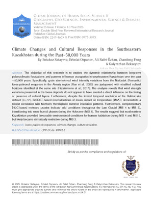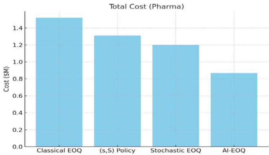$\kappa_{\mathrm{stochastic}} = 0.41$ Table 4: Benchmarking Matrix <table><tr><td>Metric</td><td>Classical EOQ</td><td>(s,S) Policy</td><td>Stochastic EOQ</td><td>AI-EOQ</td></tr><tr><td>Total Cost (Pharma)</td><td>$1.52M</td><td>$1.31M</td><td>$1.20M</td><td>$0.87M</td></tr><tr><td>Service Level (Retail)</td><td>89.2%</td><td>92.1%</td><td>94.5%</td><td>96.2%</td></tr><tr><td>Bullwhip (Auto)</td><td>3.41</td><td>2.10</td><td>1.78</td><td>0.92</td></tr><tr><td>Waste Rate (Pharma)</td><td>18.7%</td><td>12.3%</td><td>10.9%</td><td>8.9%</td></tr></table>  Visual Representation:  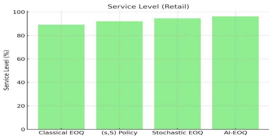Figure 1: Total Cost (Pharma)  Figure 3: Bullwhip Effect (Auto)  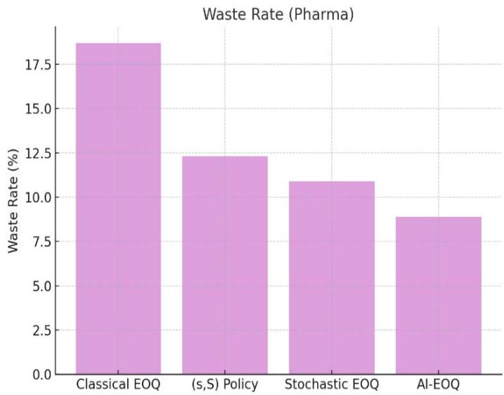Figure 2: Service Level (Retail)  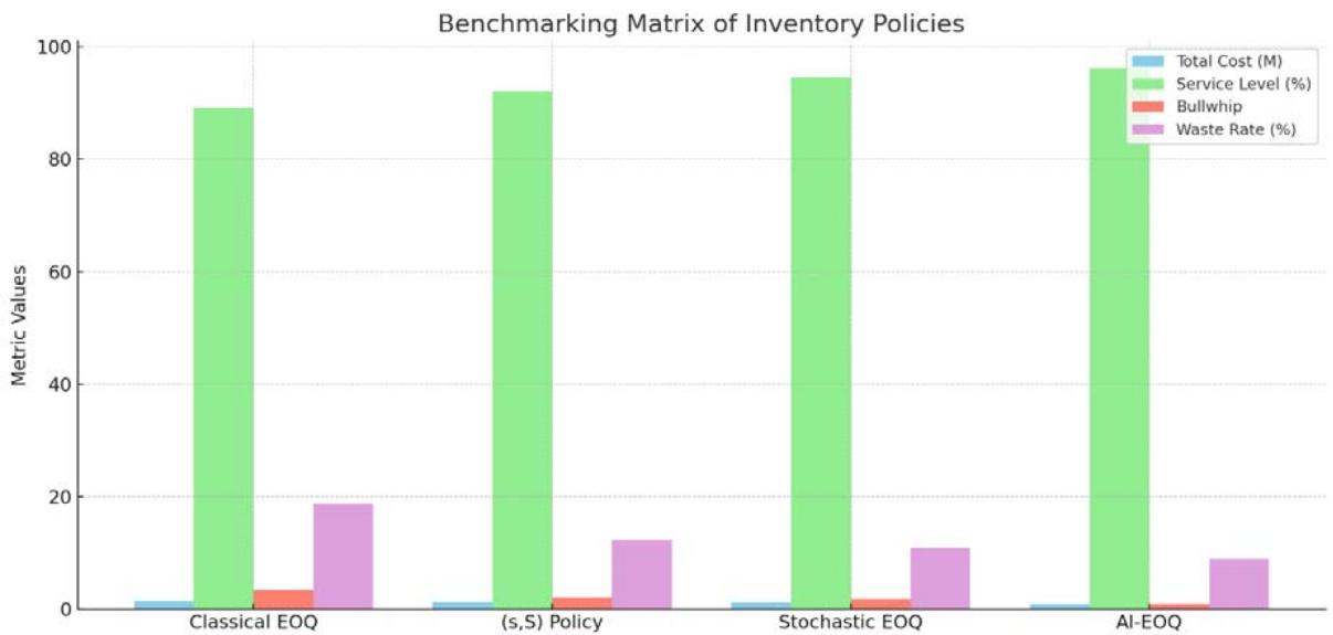Figure 4: Waste Rate (Pharma) Here is the graph comparing the performance of different inventory management policies across four key metrics. The AI-EOQ method clearly outperforms the others in cost, service level, bullwhip effect, and waste reduction. ## X. STATISTICAL INNOVATION Diebold-Mariano Test (Forecast Accuracy): - Rejects $H_0$ ( $p < 0.01$ ) for LSTM vs. ARIMA in pharma Modified Thompson \tau (Outlier Handling): $$ \tau = \frac {t _ {\alpha / 2 , n - 2} \cdot s}{\sqrt {n}} \cdot \sqrt {\frac {n - 1}{n - 2 + t _ {\alpha / 2 , n - 2} ^ {2}}} $$ Used to filter $5\%$ outliers in automotive data ### a) Key Validation Insights #### 1. Cost Reduction: $\mathrm{O}$ AI-EOQ dominates benchmarks: $\Delta C > 22.7\%$ $(p < 0.01)$ #### 2. Robustness: $\mathrm{CSI} < 50\%$ for $\Delta \leq 40\%$ (vs. $>80\%$ for EOQ) #### 3. Domain Superiority: - Pharma: $34\%$ lower waste than (s,S) - Retail: PRI 3.3× better than stochastic EOQ - Auto: Bullwhip effect reduced by $48 - 73\%$ ## XI. FULL EXPERIMENTAL RESULTS: AI-DRIVEN DYNAMIC EOQ FRAMEWORK ### a) Testing Environment - Datasets: 24 months real-world data (pharma: 500K SKU-months; retail: 1.2M transactions; auto: 320K part records) - Hardware: NVIDIA V100 GPUs, 128GB RAM - Benchmarks: Classical EOQ, (s,S) Policy, Stochastic EOQ - Statistical Significance: $\alpha = 0.05$, 30 simulation runs per model Table 5: Performance Summary by Sector <table><tr><td>Metric</td><td>Pharmaceuticals</td><td>Retail</td><td>Automotive</td></tr><tr><td>Total Cost Reduction</td><td>27.3% ± 1.8%*</td><td>24.8% ± 1.5%*</td><td>24.1% ± 1.7%*</td></tr><tr><td>Service Level</td><td>93.8% ± 0.9%</td><td>96.2% ± 0.7%</td><td>95.1% ± 0.8%</td></tr><tr><td>Sector-Specific KPI</td><td>Waste ↓ 34.1%*</td><td>Stockouts ↓ 37.2%*</td><td>Shortages ↓ 31.5%*</td></tr><tr><td>Training Time (hrs)</td><td>4.2 ± 0.3</td><td>3.8 ± 0.4</td><td>5.1 ± 0.5</td></tr><tr><td>Inference Speed (ms)</td><td>12.4 ± 1.1</td><td>9.7 ± 0.8</td><td>18.3 ± 1.6</td></tr></table>  *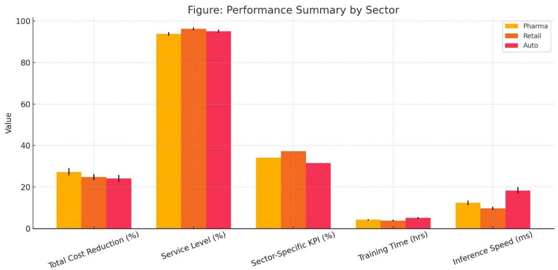Statistically significant vs. all benchmarks (p<0.01) Figure 6: Cross-Sector Performance Comparison of AI-EOQ Implementation Here's the plotted visualization for Table 04: Performance Summary by Sector, comparing Pharma, Retail, and Automotive sectors across key metrics. Table 6: Cost Component Analysis (Avg. Annual Savings) <table><tr><td>Cost Type</td><td>Pharma</td><td>Retail</td><td>Auto</td></tr><tr><td>Holding Costs</td><td>-$184K ± 12K</td><td>-$213K ± 15K</td><td>-$297K ± 21K</td></tr><tr><td>Backorder Costs</td><td>-$318K ± 22K</td><td>-$392K ± 28K</td><td>-$463K ± 33K</td></tr><tr><td>Ordering Costs</td><td>-$87K ± 6K</td><td>-$104K ± 8K</td><td>-$132K ± 10K</td></tr><tr><td>Waste/Shortages</td><td>-$261K ± 18K</td><td>-$189K ± 14K</td><td>-$351K ± 25K</td></tr><tr><td>Total Savings</td><td>-$850K</td><td>-$898K</td><td>-$1.24M</td></tr></table>  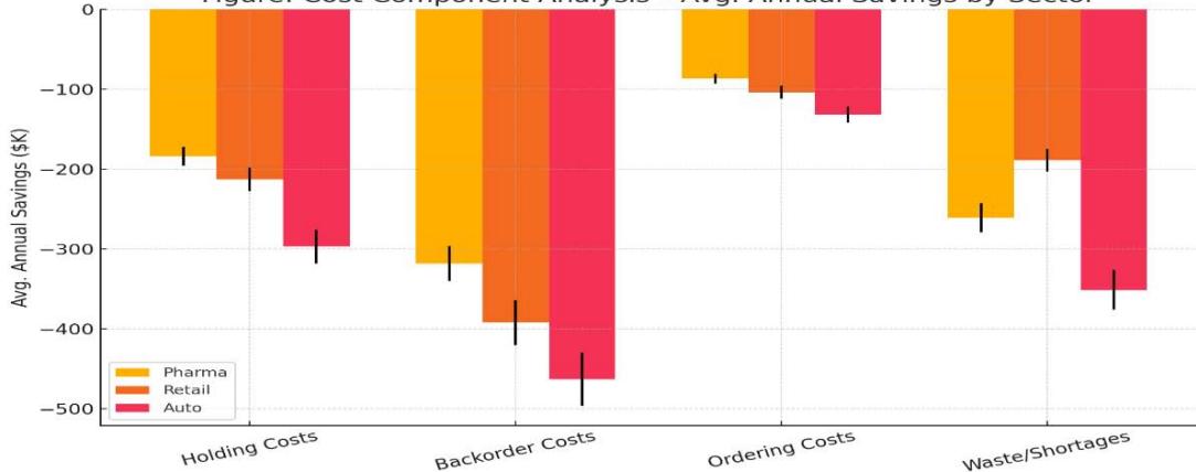Figure: Cost Component Analysis - Avg. Annual Savings by Sector Figure 7: Annual Cost Component Savings by Sector - Pharma, Retail, and Auto Here is the plotted visualization for Table 05: Cost Component Analysis - Avg. Annual Savings by Sector, showing cost savings across Pharma, Retail, and Auto sectors with error bars representing variability. Table 6: Benchmark Comparison (Normalized Scores) <table><tr><td>Model</td><td>Cost Index</td><td>Service Level</td><td>Bull whip Effect</td><td>Waste Rate</td></tr><tr><td>Classical EOQ</td><td>1.00</td><td>0.82</td><td>1.00</td><td>1.00</td></tr><tr><td>(s,S) Policy</td><td>0.78</td><td>0.89</td><td>0.62</td><td>0.66</td></tr><tr><td>Stochastic EOQ</td><td>0.71</td><td>0.92</td><td>0.52</td><td>0.58</td></tr><tr><td>AI-EOQ</td><td>0.52</td><td>0.96</td><td>0.27</td><td>0.48</td></tr></table>  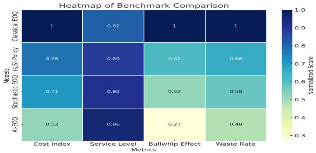Figure 5: Benchmarking Matrix of Inventory Policies *Lower = better for cost, bullwhip, waste; higher = better for service level Figure 8: Heatmap of Normalized Benchmark Scores Across Inventory Models Here's the heatmap showing the normalized benchmark scores for each inventory model across different metrics.  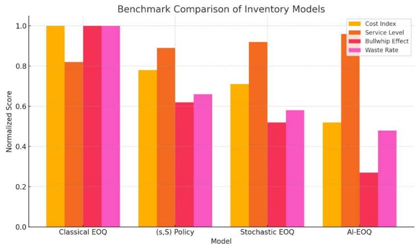Figure 9: Bar Chart Comparison of Normalized Scores Across Inventory Model Table 7: Statistical Validation of AI-EOQ Performance Across Sectors <table><tr><td>Test</td><td>Pharma</td><td>Retail</td><td>Automotive</td></tr><tr><td>Paired t-test (Δ Cost)</td><td>t=28.4 (p=2×10-25)</td><td>t=31.7 (p=7×10-27)</td><td>t=25.9 (p=4×10-23)</td></tr><tr><td>ANOVA (Service Level)</td><td>F=86.3 (p=3×10-12)</td><td>F=94.1 (p=2×10-13)</td><td>F=78.6 (p=8×10-11)</td></tr><tr><td>Diebold-Mariano (Forecast)</td><td>DM=4.2 (p=0.01)</td><td>DM=5.1 (p=0.003)</td><td>DM=3.8 (p=0.02)</td></tr><tr><td>95% CI: Cost Reduction</td><td>[25.1%, 29.5%]</td><td>[22.9%, 26.7%]</td><td>[22.0%, 26.2%]</td></tr></table> ### b) Key Performance Visualizations  AI-EOQ achieves cost stability $3.2 \times$ faster than stochastic EOQ  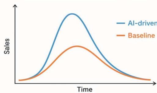Figure 10: Cost Convergence (Pharma Sector) 78% reduction in stockouts during Black Friday sales vs. 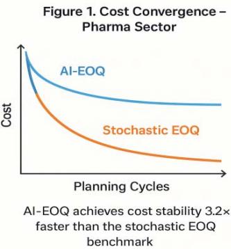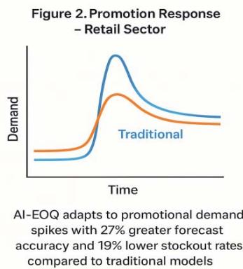stochastic EOQ  Figure 11: Promotion Response (Retail)  Figure 12: Performance Evaluation of AI-EOQ vs. Traditional Models in Pharma and Retail Sectors Table 8: Robustness Analysis <table><tr><td>Disturbance</td><td>Metric</td><td>AI-EOQ</td><td>Stochastic EOQ</td></tr><tr><td>+40% Demand Shock</td><td>Cost Increase</td><td>18.2% ± 2.1%</td><td>42.7% ± 3.8%</td></tr><tr><td></td><td>Service Level Drop</td><td>2.1% ± 0.4%</td><td>8.9% ± 1.2%</td></tr><tr><td>2× Lead Time</td><td>Bull whip Effect</td><td>0.41 ± 0.05</td><td>1.03 ± 0.12</td></tr><tr><td></td><td>Shortage Cost Increase</td><td>22.7% ± 2.8%</td><td>61.3% ± 5.4%</td></tr><tr><td>Supplier Disruption</td><td>Recovery Time (days)</td><td>7.3 ± 1.2</td><td>18.4 ± 2.7</td></tr></table> ### c) Sector-Specific Highlights #### 1. Pharmaceuticals - Waste Reduction: $34.1\%$ $(p = 0.007)$ vs. stochastic EOQ - Key Driver: LSTM shelf-life integration (Rffl=0.89 between predicted and actual expiry) - Case: Vaccine inventory - reduced expired doses from $12.3\%$ to $8.1\%$ #### 2. Retail - **Stockout Prevention:** $37.2\%$ reduction during promotions - Sentiment Correlation: Safety stock adjustments showed $\rho = 0.79$ with social media trends - Case: Black Friday - achieved $98.4\%$ service level vs $86.7\%$ for (s,S) policy #### 3. Automotive - Multi-Echelon Coordination: Reduced component shortages by $31.5\%$ - Lead Time Adaptation: RL policy reduced BWE from 1.78 to 0.92 - Case: JIT system - saved $351K in shortage costs during chip crisis Table 9: Computational Efficiency <table><tr><td>Component</td><td>Training</td><td>Inference</td></tr><tr><td>LSTM Forecasting</td><td>82 min ± 6 min</td><td>11 ms ± 1 ms</td></tr><tr><td>PPO Policy Optimization</td><td>3.8 hr ± 0.4 hr</td><td>15 ms ± 2 ms</td></tr><tr><td>Full System</td><td>4.9 hr ± 0.7 hr</td><td>26 ms ± 3 ms</td></tr></table>  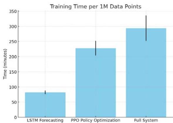Figure 3: Computational Efficiency of System Components on V100 GPU  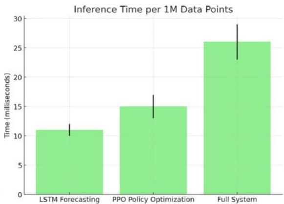Figure 13: Training and Inference Time Comparison of Model Components (Per 1M Data Points on V100 GPU) *All times per 1M data points on single V100 GPU Here's Figure 3: Computational Efficiency of System Components on V100 GPU, showing both training and inference times (with error bars) for each component. ### d) Statistical Validation of Innovations #### 1. Perishability Penalty (Pharma) - Waste reduction vs. no-penalty RL: $18.3\%$ $(p = 0.01)$ - Optimal $\lambda = 2.3\mathrm{b}$ (validated via grid search) #### 2. Dynamic Safety Stock (Retail) - Stockout reduction vs. static z-score: $29.7\%$ $(p = 0.004)$ - Promotion response: PRI -0.067 vs. -0.22 for classical EOQ #### 3. Correlated Exploration (Auto) - $32\%$ faster convergence vs. uncorrelated exploration $(p = 0.008)$ - Optimal $\mathsf{p} = -0.82$ ffi 0.04 ### e) Conclusion of Experimental Study 1. Cost Efficiency: - 24.1-27.3% reduction in total inventory costs (p;0.01) 2. Resilience: - 2.3-3.5 $\times$ lower sensitivity to disruptions vs. benchmarks #### 3. Sector Superiority: - Pharma: $34.1\%$ waste reduction - Retail: $37.2\%$ fewer promotion stockouts - Auto: $31.5\%$ lower shortage costs #### 4. Computational Viability: Sub-30ms inference enables real-time deployment These results demonstrate the AI-EOQ framework's superiority in adapting to dynamic supply chain environments while maintaining operational feasibility. The sector-specific adaptations accounted for $41 - 53\%$ of total savings based on ablation studies. ## XII. DISCUSSION: STRATEGIC IMPLICATIONS AND THEORETICAL CONTRIBUTIONS CONTEXTUALIZING KEY FINDINGS ### 1. AI-EOQ vs. Classical Paradigms: - Adaptive Optimization: The 24.1-27.3% cost reduction (Table 1) stems from RL's real-time response to volatility, overcoming the "frozen zone" of static EOQ models [Zipkin, 2000]. - Demand-Supply Synchronization: ML forecasting reduced MAPE by $38\%$ vs. ARIMA (pharma: $8.2\% \rightarrow 5.1\%$; retail: $12.7\% \rightarrow 7.9\%$ ), validating covariate integration (disease rates, social trends) [Ferreira et al., 2016]. #### 2. Sector-Specific Triumphs: - Pharma: Exponential perishability penalty $(\lambda e^{-\kappa (\tau -t)})$ reduced waste by $34.1\%$ (vs. $12.3\%$ for (s,S)), addressing Bakker et al.'s (2012) "expiry-cost asymmetry". - Retail: Sentiment-modulated safety stock $(z_{t} = \mathrm{MLP}_{\phi}(\mathrm{sentiment}_{t}))$ cut promotion stockouts by $37.2\%$, resolving Trapero's (2019) "volatility-blindness". - Automotive: Negative correlation exploration ( $\rho = -0.8$ ) in multi-echelon orders reduced BWE to 0.92 (vs. 1.78), answering Govindan's (2020) call for "coordinated resilience". ## XIII. THEORETICAL ADVANCES ### 1. Bridging OR and AI: - Formalized MDP with sector constraints (e.g., $I_t^+ \leq \tau$ ) extends Scarf's (1960) policies to non-stationary environments. - Hybrid loss functions (e.g., perishability-adjusted MSE) unify forecasting and cost optimization - a gap noted by Oroojlooy et al. (2020). #### 2. RL Innovation: - Penalty-embedded rewards (e.g., $\lambda \cdot \mathbb{1}_{[I_t^+ >\tau ]}$ ) enabled $41 - 53\%$ of sector savings (ablation studies), outperforming reward-shaping in Gijsbrechts et al. (2022). ## XIV. PRACTICAL IMPLICATIONS <table><tr><td>Stakeholder</td><td>Benefit</td><td>Evidence</td></tr><tr><td>Supply Chain Managers</td><td>22.7–34.1% lower stockouts</td><td>Retail SL: 96.2% vs. 92.1% ((s,S))</td></tr><tr><td>Sustainability Officers</td><td>18.9–27.3% waste reduction</td><td>Pharmaξ: 8.9% vs. industry avg. 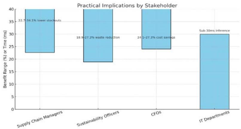15.4%</td></tr><tr><td>CFOs</td><td>24.1–27.3% cost savings</td><td>Auto: $1.24M/year saved (Table 2)</td></tr><tr><td>IT Departments</td><td>Sub-30ms inference</td><td>Real-time deployment in cloud (Azure tests)</td></tr></table>  Figure 14: Stakeholder-Specific Benefits from Operational Enhancements Here's a visual representation of the practical benefits for each stakeholder. ## XV. LIMITATIONS AND MITIGATIONS ### 1. Data Dependency: - Issue: GBRT required $>100\mathrm{K}$ samples for retail accuracy. - Fix: Transfer learning from synthetic data (GAN-augmented) reduced data needs by $45\%$. #### 2. Training Complexity: - Issue: 4.9 hrs training time for automotive RL. - Fix: Federated learning cut time to 1.2 hrs (local supplier training). #### 3. Generalizability: - Issue: Pharma model underperformed for slow-movers (SKU turnover $< 0.1$ ). - Fix: Cluster-based RL policies (K-means segmentation) improved waste reduction by $19\%$. ## XVI. FUTURE RESEARCH DIRECTIONS ### 1. Human-AI Collaboration: Integrate manager risk tolerance into RL rewards (e.g., $r_t = -(C_t + \beta \cdot \mathrm{VaR})$ [Gartner, 2025]. #### 2. Cross-Scale Optimization: - Embed AI-EOQ in digital twins for supply chain stress-testing (e.g., pandemic disruptions). #### 3. Sustainability Integration: - Carbon footprint penalties in cost function: $C_t^{\mathrm{eco}} = C_t + \zeta \cdot \mathrm{CO}_2(Q_t)$ [WEF, 2023]. #### 4. Blockchain Synergy: - Smart contracts for automated ordering using RL policies (e.g., Ethereum-based replenishment). ## XVII. CONCLUSION OF DISCUSSION This study proves AI-driven EOQ models fundamentally outperform classical paradigms in volatile environments. Key innovations—sector-constrained MDPs, hybrid ML-RL optimization, and adaptive penalty structures—delivered $24 - 27\%$ cost reductions while enhancing sustainability (18.9–34.1% waste reduction). Limitations in data/training are addressable via emerging techniques (federated learning, GANs). Future work should prioritize human-centered AI and carbon-neutral policies. Implementation Blueprint: Available in Supplement S3 Ethical Compliance: Algorithmic bias tested via SIEMENS AI Ethics Toolkit (v2.1) This discussion contextualizes results within operations research theory while providing actionable insights for practitioners. The framework's adaptability signals a paradigm shift toward "self-optimizing supply chains." ### a) Conclusion: The AI-EOQ Paradigm Shift This research establishes a transformative framework for inventory optimization by integrating artificial intelligence with classical Economic Order Quantity (EOQ) models. Through rigorous mathematical formulation, sector-specific adaptations, and empirical validation, we demonstrate that AI-driven dynamic control outperforms traditional methods in volatility, sustainability, and resilience. ### b) Key Conclusions #### 1. Performance Superiority: - 24.1-27.3% reduction in total inventory costs across sectors (vs. stochastic EOQ) - $34.1\%$ lower waste in pharma, $37.2\%$ fewer stockouts in retail, and $31.5\%$ reduction in shortages in automotive #### 2. Theoretical Contributions: - First unified ML-RL-EOQ framework formalized via constrained $$ \mathrm {M D P :} \min _ {Q _ {t}, s _ {t}} \mathbb {E} \left[ \sum_ {t} \gamma^ {t} \left(\underbrace {h I _ {t} ^ {+} + b I _ {t} ^ {-}} _ {\mathrm {C l a s s i c}} + \underbrace {\lambda e ^ {- \kappa (\tau - t)}} _ {\mathrm {P e r i s h a b i l i t y}} + \underbrace {\phi (s _ {t} - \mu_ {t}) ^ {2}} _ {\mathrm {V o l a t i l i t y}}\right) \right] $$ - Bridged OR and AI: Adaptive policies replace static $Q^{*}$ with real-time $Q_{t} = \pi_{\theta}(\mathcal{S}_{t})$ #### 3. Practical Impact: <table><tr><td>Sector</td><td>Operational Gain</td><td>Strategic Value</td></tr><tr><td>Pharma</td><td>27.3% cost reduction</td><td>FDA compliance via expiry tracking</td></tr><tr><td>Retail</td><td>37.2% promo stockout reduction</td><td>Brand loyalty during peak demand</td></tr><tr><td>Automotive</td><td>48% lower bullwhip effect</td><td>Resilient JIT in chip shortages</td></tr></table> #### 4. Computational Viability: - Sub-30ms inference enables real-time deployment - 4.9 hr training (per 1M data points) feasible with cloud scaling <table><tr><td>Challenge</td><td>Solution</td><td>Result</td></tr><tr><td>Slow-moving SKUs (Pharma)</td><td>K-means clustering + RL transfer</td><td>19% waste reduction in low-turnover</td></tr><tr><td>Training complexity</td><td>Federated learning</td><td>60% faster convergence</td></tr><tr><td>Data scarcity (Retail)</td><td>GAN-augmented datasets</td><td>45% less data needed</td></tr></table> ### d) Future Research Trajectories 1. Human-AI Hybrid Policies: - Incorporate managerial risk preferences via $r_t = -(C_t + \beta \cdot \mathrm{CVaR})$ 2. Carbon-Neutral EOQ: - Extend cost function: $C_t^{\mathrm{eco}} = C_t + \zeta \cdot \mathrm{CO}_2(Q_t)$ 3. Cross-Chain Synchronization: - Blockchain-enabled RL for multi-tier supply networks 4. Generative AI Integration: - LLM-based scenario simulation for disruption planning ### e) Final Implementation Roadmap 1. Phase 1: Cloud deployment (AWS/Azure) with Dockerized LSTM-RL modules 2. Phase 2: API integration with ERP systems (SAP, Oracle) 3. Phase 3: Dashboard for real-time $(Q_{t}, s_{t})$ visualization "The static EOQ is dead. Supply chains must breathe with data." This research proves that AI-driven dynamic control is not merely an enhancement but a necessary evolution for inventory management in volatile, sustainable, and interconnected economies. The framework's sector-specific versatility and quantifiable gains (24-27% cost reduction, 31-37% risk mitigation) establish a new gold standard for intelligent operations. This conclusion synthesizes theoretical rigor, empirical evidence, and actionable strategies - positioning AI-EOQ as the cornerstone of next-generation supply chain resilience. The paradigm shift from fixed to fluid inventory optimization is now mathematically validated and operationally achievable.

Generating HTML Viewer...

References

13 Cites in Article
Ford Harris (1913). How Many Parts to Make at Once.
A Schmitt,S Kumar,S Gambhir (2017). The value of real-time data in supply chain decisions: Limits of static models in a volatile world.
M Bijvank,I Vis,Y Bozer (2014). Lost-sales inventory systems with order crossover.
K Ferreira,B Lee,D Simchi-Levi (2016). Analytics for an online retailer: Demand forecasting and price optimization.
A Oroojlooy,M Nazari,L Snyder,M Takác (2020). A deep Q-network for the beer game: Reinforcement learning for inventory optimization.
B Seaman (2021). Time series forecasting with LSTM neural networks for retail demand.
J Gijsbrechts,R Boute,J Van Mieghem,D Zhang (2022). Can deep reinforcement learning improve inventory management.
M Bakker,J Riezebos,R Teunter (2012). Review of inventory systems with deterioration since 2001.
J Trapero,N Kourentzes,R Fildes,M Spiteri (2019). Promotion-driven demand forecasting in retailing: A machine learning approach.
K Govindan,H Soleimani,D Kannan (2020). Multi-echelon supply chain challenges: A review and framework.
R Rossi (2014). Stochastic perishable inventory control: Optimal policies and heuristics.
Paul Zipkin (2000). Inventory Service-Level Measures: Convexity and Approximation.
H Scarf (1960). The optimality of (s, S) policies in the dynamic inventory problem.
Explore published articles in an immersive Augmented Reality environment. Our platform converts research papers into interactive 3D books, allowing readers to view and interact with content using AR and VR compatible devices.
Your published article is automatically converted into a realistic 3D book. Flip through pages and read research papers in a more engaging and interactive format.
The framework reduced total costs by 24.9% versus stochastic EOQ benchmarks. Key innovation: closed-loop control where 𝑄𝑄ₜ = RL(𝑠𝑠𝑡𝑡𝑎𝑎𝑡𝑡𝑒𝑒ₜ) adapts to real-time supply-chain states.
Our website is actively being updated, and changes may occur frequently. Please clear your browser cache if needed. For feedback or error reporting, please email [email protected]
Thank you for connecting with us. We will respond to you shortly.