I. INTRODUCTION

Network models are one in every of the most effective studies that apply to a vast type of decision problems that can be modeled as networks optimization problems and solved with efficiency and effectiveness. The family of network optimization problems includes the; max flow, transportation problem, and min-cost flow problems. These problems are simply expressed by using a network of edges, and vertices. Transportation Network and Graph theory are the two major elementary application areas of Mathematics. Transportation Network models and graphs play a very important role in Optimizing techniques, Network analysis, Network-flow theory is one of the best-studied and developed fields of optimization, and has important relations to quit completely different fields of science and technology such as combinatorial mathematics, algebraical topology, circuit theory, geographic info systems(GIS), VLSI design, and so forth, etc, besides standard applications to transportation, scheduling, etc. in operations research.

In 2005, Antonievella[1] initiate and introduced the foundations of topological properties on graph theory. Consequently, Vimala and Kalpana [5] developed the concept named Bipartite Graph and applied it in Matching and Coloring. In recently, 2019, Introduced Topological solution of a Transportation problem using Topologized

Graph by Santhi et al. In 2015, Kadhim et al. An Approach for solving Transportation Problem Using Modified Kruskal's Algorithm. In a network with unit transportation cost on the edges, the problem is to determine the maximum possible flow from the source to the demand. Also, Transportation problems link along with the factors of production during an advanced net of relationships between producers and consumers. The result is usually a more effective division of production by the exploitation of comparative geographical ideal conditions, similarly as the best approach to make economies of scale and scope.

The productivity of space, capital, and labor is therefore increased with the efficiency of distribution and personal mobility. The economic process is progressively connected with transport developments, namely infrastructures, but also with managerial expertise, which is crucial for logistics.

The Transportation Problem (TP) is also one of the highly regarded problems in the field of optimization in which the objective is to minimize the total transportation cost of distributing resources from several sources to some destinations. It has numerous applications in the real world. Hitchcock is responsible for formulating the TP as a mathematical model. The Hitchcock-Koopmans transportation problem, or basically the transportation problem is to compute an assignment with a minimum possible cost. To handle a transportation problem, the decision parameters, for example, availability, requirement, and therefore the unit transportation cost of the model. Many of the researchers mentioned and introduced so many methods to find the optimal solution to a Transportation problem.

Many researchers have made numerous attempts to find an IBFS such as Northwest Corner Method, Minimum Cost Method, VAM -Vogel's Approximation Method, MODI Method, and Stepping Stone Method which are all heuristic in nature. In this study, we attempted to solve the TP using a Bipartite graph to enhance the convergence rate to reach a promising optimal solution. This algorithm is also heuristic in nature but less complicated in the implementation compared to many existing heuristic algorithms.

II. MATHEMATICAL FORMULATION OF THE TRANSPORTATION PROBLEM

Let us assume that in general that a particular product is manufactured in m production plants known as sources denoted by $S_1,S_2,\dots ,S_m$ with respective capacities $a_1,a_2,\dots ,a_m$, and total distributed to n distribution centers known as sinks denoted by $D_1,D_2,\dots ,D_m$ with respective demands $b_1,b_2,\dots ,b_n$. Aso, assume that the transportation cost from $i^{th}$ -source to the $j^{th}$ -sink is unit transportation cost $e_{ij}$ and the amount shipped is $X_{ij}$, where $i=1,2,\dots ,m$ and $j=1,2,\dots ,n$.

Mathematical Model:

The total transportation cost is

Minimize $\sum _{i=1}^m\sum _{j=1}^n{X}_{ij}{e}_{ij}$

Subject to the constraints i. $\sum _{j=1}^n{X}_{ij}=a_i,$ $i=1,2,\dots ,m$

ii. $\sum _{i=1}^m{X}_{ij}=b_j$, $j=1,2,\dots ,n$ and iii. $X_{ij}\ge 0$ for all $i=1,2,\dots ,m$ and $j=1,2,\dots ,n$

Note that here the sum of the supplies equals the sum of the demands. i.e. $\sum _{i=1}^m{a}_i=\sum _{j=1}^n{b}_j$. Such problems are called balanced transportation problems and otherwise, i.e. $\sum _{i=1}^m{a}_i\ne \sum _{j=1}^n{b}_j$, known as unbalanced transportation problems.

i.

ii.

Introduce a dummy origin in the transportation table; the cost associated with this origin is set equal to zero. The availability at this origin is: $\sum _{i=1}^m{a}_i-\sum _{j=1}^n{b}_j=0$.

III. PROPOSED ALGORITHM TO SOLVE THE TP

The proposed method can be applied to solve balanced and unbalanced TPs.

Step 1: Verify the given transportation problem is balanced or unbalance.

Step 2: If the problem is unbalanced transportation problem by introducing dummy row(s) or dummy column(s) with zero transportation cost.

Step 3: Draw the graph of the transportation problem dependent on the situation of the supplies and demands for the graphical representation of the transportation problem.

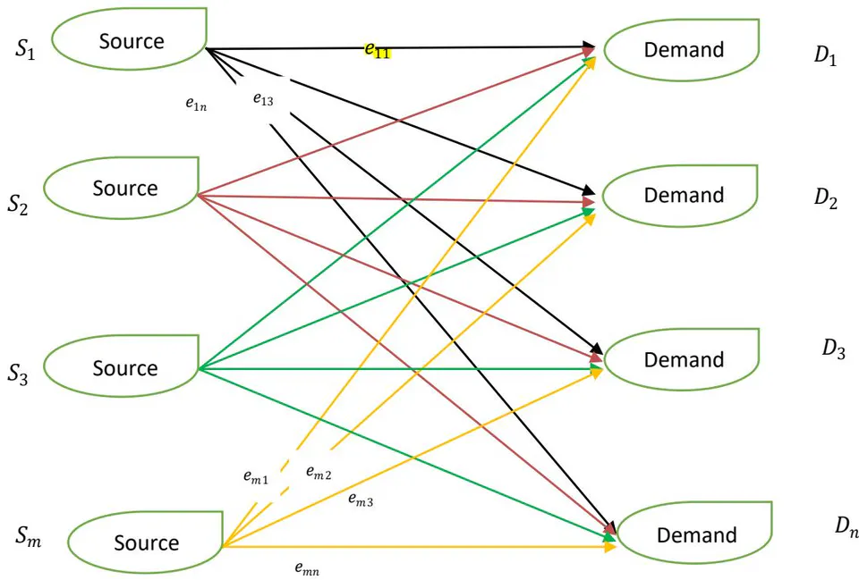
Step 4: Now selected bipartite graph which every Supply and demand of the graph has two minimum unit cost.

Step 5: Identify edges should have the minimum unit cost $e_{ij}$ (unit transportation cost) in the above step and first allocated $\text{mini}(a_i,b_j)$ most least unit cost edge.

Step 6: Start the allocation from which edge has the minimum transportation cost and reduce the minimum value from the supply vertex and demand vertex with satisfies boundary condition of the bipartite graph.

Step 7: If it satisfies the two conditions of graph go to the next step.

Step 8: Identify edges should have the minimum unit cost $e_{ij}$ (unit transportation cost) in above step and first allocated $\text{mini}(a_i,b_j)$ most least unit cost edge of above step, and reduce the minimum value from the supply vertex and demand vertex with satisfies boundary condition of the bipartite graph.

IV. A COMPARISON OF THE METHODS

The comparisons of the results are studied in this research to measure the effectiveness of the proposed method. The detailed representation of the numerical data of Table I. is provided in Appendix I.[4].

	TCIFS						% increase	from	the	minimal	total cost
Ahamd et al..(2016)	NWCM	LCM	VAM	IAM	BA	OPTIMAL	NWCM	LCM	VAM	IAM	NEWA
BTP-1	1,500	1,450	1,500	1,390	1,390	1,390	7.91	4.31	7.91	0.00	0.00
BTP-2	226	156	156	156	156	156	44.87	0.00	0.00	0.00	0.00
BTP-3	234	191	187	186	183	183	27.87	4.37	2.18	1.64	0.00
BTP-4	4,285	2,455	2,310	2,365	2,170	2,170	97.46	13.13	6.45	8.99	0.00
BTP-5	3,180	2,080	1,930	1,900	1,900	1,900	67.37	9.47	1.58	0.00	0.00
UTP-1	1,815	1,885	1,745	1,695	1,655	1,650	10.0	14.24	5.76	2.73	0.30
UTP-2	18,800	8,800	8,350	8,400	7,100	7,100	142.6	13.55	7.74	8.39	0.00
UTP-3	14,725	14,625	13,225,	13,075	12,475	12,475	18.04	17.23	6.01	4.80	0.00
UTP-4	13,100	9,800	9,200	9,200	9,200	9,200	42.39	6.52	0.00	0.00	0.00
UTP-5	8,150	6,450	6,000	5,850	5,600	5,600	45.53	15.18	7.14	4.46	0.00

Radar graphs for the percentage deviation (of the NWCM, MC, VAM,TDM,TDSM, VAM) with New method(BA) from minimal total cost solution) obtained in Table I are presented in Figure 2.

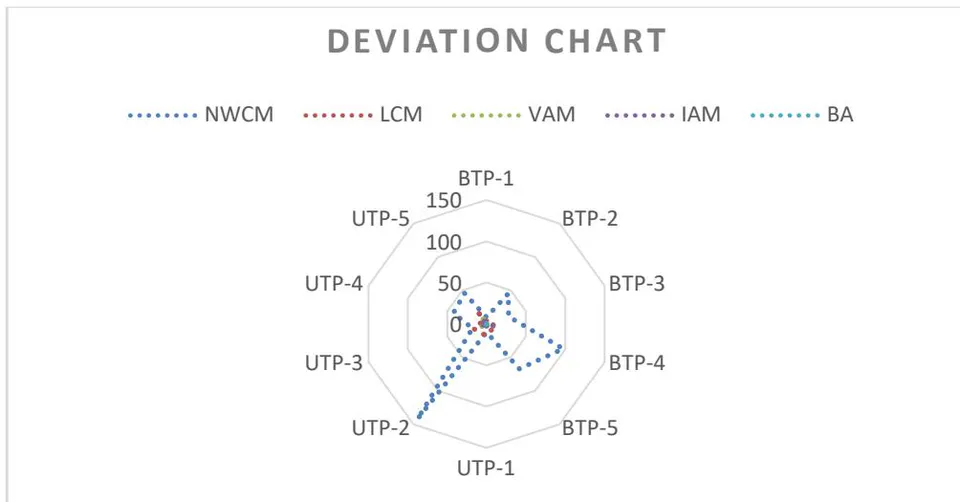
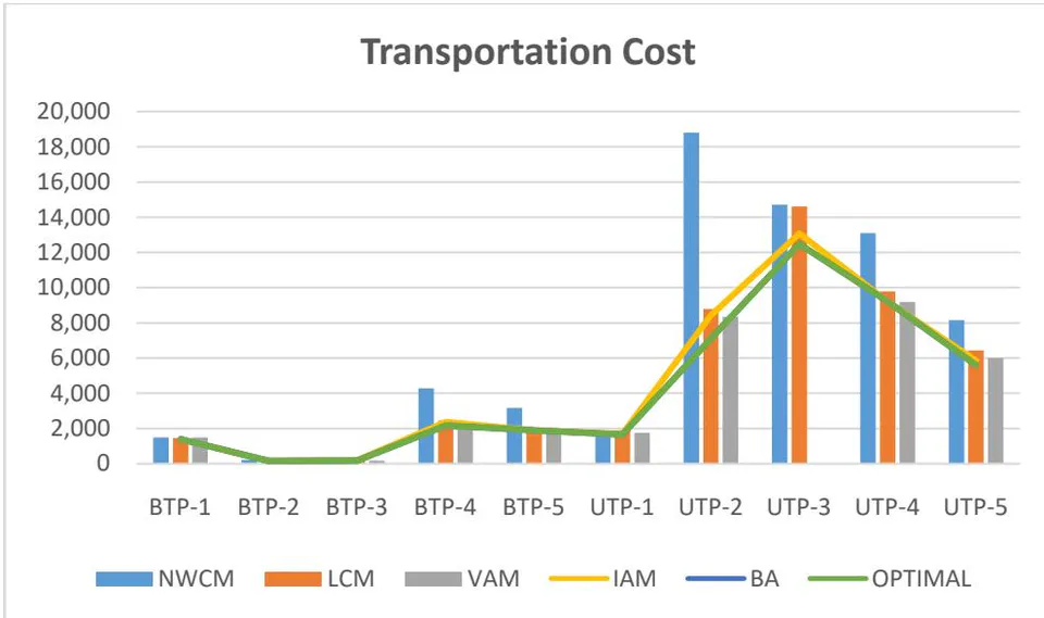
It can easily be observed the above results (Table 1, Figure 2 and Figure 3), new method yields better results to all the problems in Table 1 compared with NWCM, LCM, VAM and IAM.

Next comparative results obtained by NWCM, LCM, VAM, MODI and New method for the one benchmark instances is shown in the following Table II. (Kenan Karagul and Yusuf Sahin).

Destination/ Sources	$D_1$	$D_2$	$D_3$	$D_4$	$D_5$	Su.
$S_1$	73	40	9	79	20	8
$S_2$	62	93	96	8	13	7
$S_3$	96	65	80	50	65	9
$S_4$	57	58	29	12	87	3
$S_5$	56	23	87	18	12	5
Dem.	6	8	10	4	4

The comparisons of the results are studied in this research to measure the effectiveness of the proposed method. The detailed representation of the numerical data of Table II. is provided in Appendix I.[4].

Ref

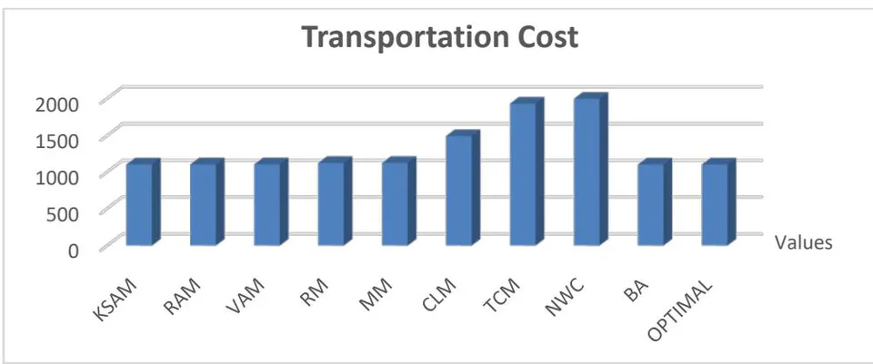
Solution Method	Values	Deviation from optimal solution(%)
KSAM	1,102	0.00
RAM	1.104	0.18
	1,104	0.18
RM	1.123	1.90
MM	1,123	1.90
CLM	1,491	35.29
TCM	1,927	74.86
NWC	1,994	80.94
BA	1,102	0.00
OPTIMAL	1,102	-

The comparative results obtained in Table II are also depicted using bar graphs and the results are given in

Figure 1 V. COMPUTATIONAL RESULTS (PROBLEM CHOOSE FROM SANTHI ET AL)

Example1.

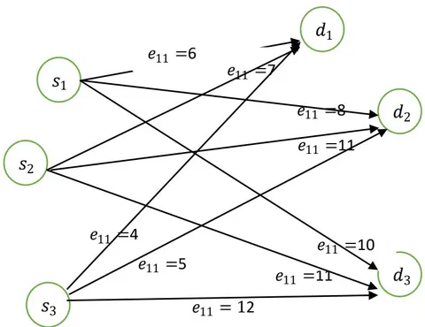
A transport company is planning to allocate owned vehicles to cities A, B and C. Here are the transport tables that have been prepared by managers of the company which gives the transportation cost from warehouses (Supply Points) to the cities(Demand Points).

	A	B	C	Supply
1	6	8	10	150
2	7	11	11	175
3	4	5	12	275
Demand	200	100	300

Step 2 Step 3.

Step 4.

Step 5

Step 6

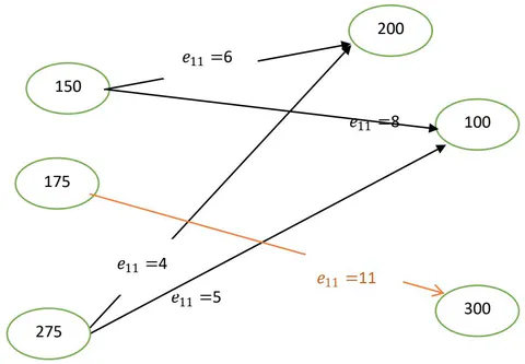
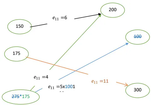
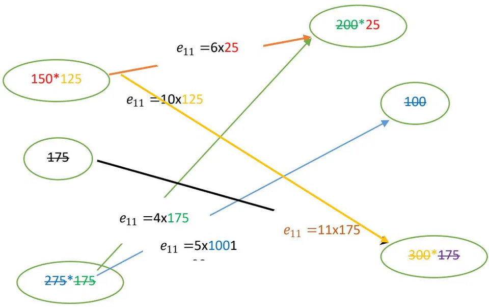
Santhi method = 4,550

Optimal solution = 4,525

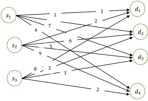
Example 2. A company manufactures motor cars and it has three factories F1, F2 and F3 whose weekly production capacities are 300, 400 and 500 pieces of cars respectively. The company supplies motor cars to its four showrooms located at d1, d2, d3 and d4 whose weekly demands are 250, 350, 400 and 200 pieces of cars respectively. The transportation costs per piece of motor cars are given in the following transportation Table. Find out the schedule of shifting of motor cars from factories to showrooms with minimum cost:

	$d_1$	$d_2$	$d_3$	$d_4$
$s_1$	3	1	7	4	300
$s_2$	2	6	5	9	400
$s_3$	8	3	3	2	500
	250	350	400	200

Step 3 Step 4

Step 5 Step 6

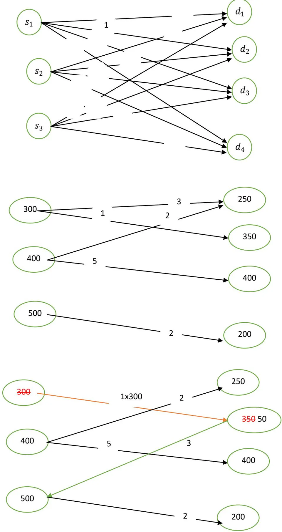
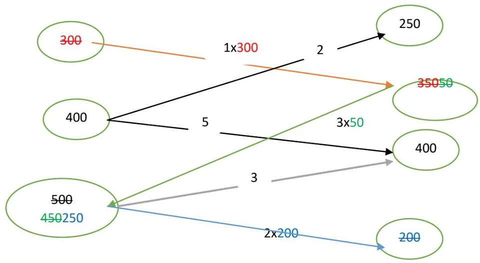
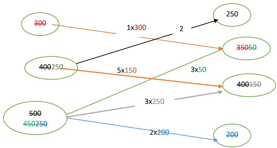
Step 7

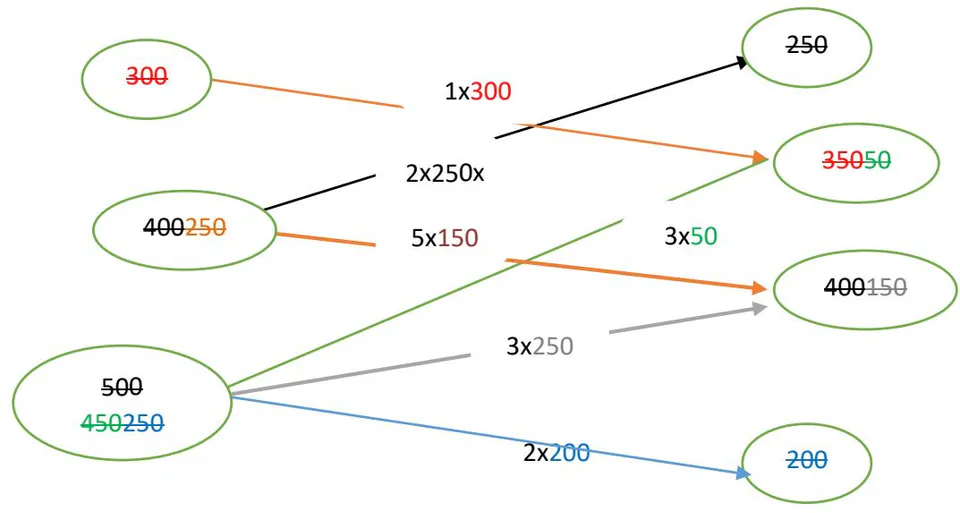
Santhi method=2,850

Optimal solution=2,850

Based on the above results new method (BA) better than other approaches.

VI. CONCLUSION

In this study, a new approach for attaining the optimal solution of a transportation problem using the Bipartite graph. Different techniques have been developed in the literature for solving the transportation problem but this approach plays an important role among topology, transportation, and graph. The comparative assessments of the above different cases show that the bipartite algorithm is efficient as compared to the studied approaches of this paper in terms of the quality of the solution. This innovative approach consumes less computational time and minimum steps to find the optimal solution to the transportation problem compared with the existing methods. However, This new method is based on the allocation of transportation costs in the transportation matrix and can be applied to all balance and unbalance transportation problems, using more variables. Hence, the comparative assessments of the above different cases show that the bipartite algorithm is efficient as compared to the studied approaches of this paper in terms of the quality of the solution. Therefore, perhaps this method will be interested in future works in real topological transportation problems, and graph and topological transportation problems are interrelationships.

APPENDIX I

Problem	Data of the problem
BTP-1	$c_{ij}=[4,3,5;6,5,4;8,10,7],s_i=[90,80,100],d_j=[70,120,80]$
BTP-2	$c_{ij}=[4,6,9,5;2,6,4,1;5,7,2,9],s_i=[16,12,15],d_j=[12,14,9,8]$
BTP-3	$c_{ij}=[5,7,10,5,3;8,6,9,12,14;10,9,8,10,15],s_i=[5,10,10],d_j=[3,3,10,5,4]$
BTP-4	$c_{ij}=[12,4,13,18,9,2;9,16,10,7,15,11;4,9,10,8,9,7;9,3,12,6,4,5;7,11,15,18,2,7;16,8,4,5,1,10],s_i=[120,80,50,90,100,60],d_j=[75,85,140,40,95,65]$
BTP-5	$c_{ij}=[12,7,3,8,10,6,6;6,9,7,12,8,12,4;10,12,8,4,9,9,3;8,5,11,6,7,9,3;7,6,8,11,9,5,6,]s_i=[60,80,70,100,90],d_j=[20,30,40,70,60,80,100]$
UTP-1	$c_{ij}=[6,10,14;12,19,21;15,14,17],s_i=[50,50,50],d_j=[30,40,55]$
UTP-2	$c_{ij}=[10,8,4,3;12,14,20,2;6,9,23,25],s_i=[500,400,300],d_j=[250,350,600,150]$
UTP-3	$c_{ij}=[12,10,6,13;19,8,16,25;17,15,15,20;23,22,26,12],s_i=[150,200,600,225],d_j=[300,500,75,100]$
UTP-4	$c_{ij}=[5,8,6,6,3;4,7,7,6,5;8,4,6,6,4],s_i=[800,500,900],d_j=[400,400,500,400,800]$
UTP-5	$c_{ij}=[5,4,8,6,5;4,5,4,3,2;3,6,5,8,4],s_i=[600,400,1,000],d_j=[450,400,200,250,300]$