
I. INTRODUCTION
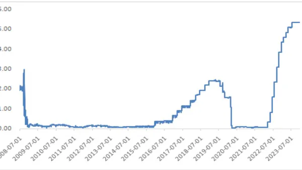
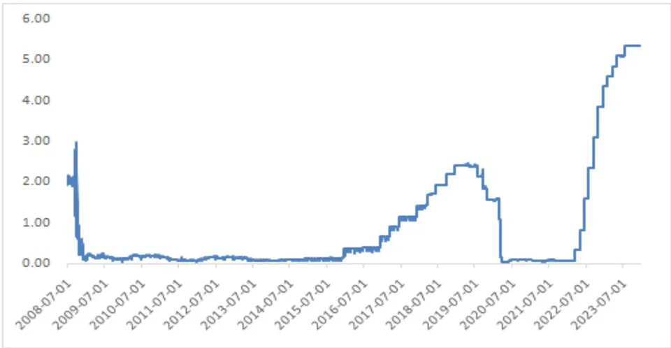
When the nominal interest rate approaches zero, entering Keynes' liquidity trap, the country's Zero Lower Bound (ZLB) renders traditional monetary policy largely ineffective. Unconventional monetary policy assumes a crucial role in releasing liquidity within the United States, as well as in regulating both the national and global economies. Following the financial crisis of 2008, the Federal funds rate persisted at or near 0, as depicted in Figure 1.
Source: WIND database
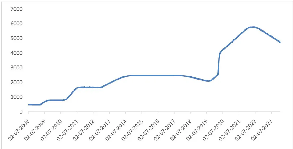
Since the benchmark interest rate plummeted swiftly in the latter half of 2008, the effective federal funds rate lingered close to zero from early 2009 until mid-2016. Throughout this interval, the Federal Reserve adopted unconventional monetary policy (UMP) measures. For instance, the Fed augmented its portfolio by acquiring Mortgage-Backed Securities (MBS) and medium-to-long-term U.S. Treasury bonds, employing methods such as Large-Scale Asset Purchases (LSAP), as illustrated in Figure 2. Additionally, the Fed employed forward guidance strategies.
Source: https://fred.stlouisfed.org/series/TREAST
Data indicates a correlation between expansionary unconventional monetary policy (UMP) and capital inflows into Emerging Markets (EM). Figure 3 illustrates the monthly percentage flows of bond funds directed towards emerging market countries.
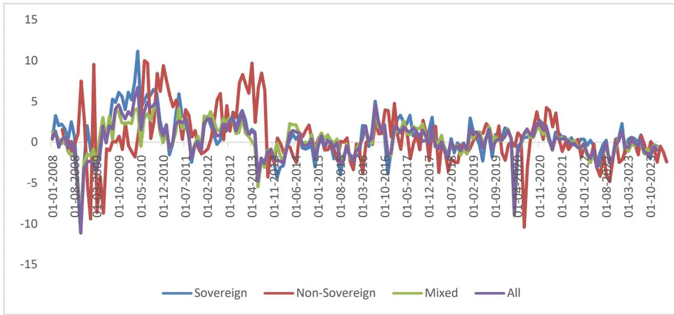
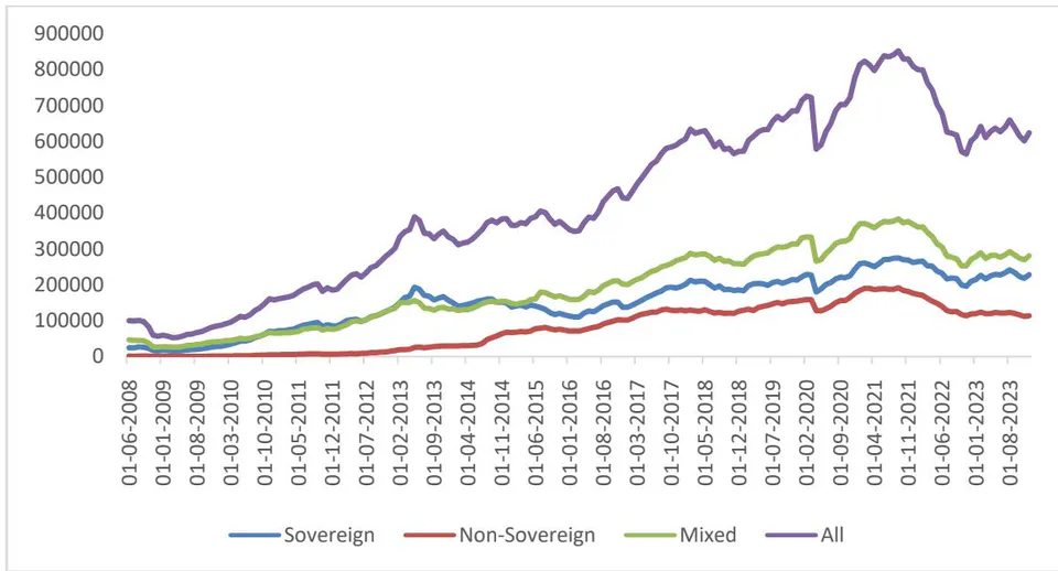
Source: EPFR Database As depicted in the figure, emerging market countries primarily witnessed capital inflows from the second half of 2008 to the first half of 2013, followed by net outflows from 2013 until the conclusion of 2016, with subsequent periods marked by substantial fluctuations. Notably, during the COVID-19 pandemic in 2020, emerging markets experienced a net inflow, transitioning to a net outflow after 2022. Figures 4-6 illustrate the total
assets of bond funds invested in Emerging Markets (EM).
Source: EPFR Database
Due to differences in ownership nature and overall volume, non-sovereign funds exhibit higher profitability requirements, resulting in greater volatility in their total assets compared to sovereign funds. Additionally, non-sovereign funds are more sensitive to U.S. monetary policy changes than sovereign funds, highlighting an asymmetry in bond capital flows. For instance, based on Figure 4, during the Federal Reserve's quantitative tightening policy since 2022, global capital shifted towards the United States, leading to significant contractions in total assets across various bond fund types compared to September 2021. By November 2022, following a 14-month decline, sovereign funds decreased by , non-sovereign funds by , and mixed funds by . Notably, the duration of these contractions is shorter than the time required for similar asset growth during easing periods. Specifically, sovereign funds took 31 months to rise, while mixed and non-sovereign funds took 51 and 70 months, respectively. Essentially, the period of ascent is five times longer than the descent period.
II. LITERATURE REVIEW
Following the collapse of the Bretton Woods system, scholarly attention has predominantly focused on the actions of the Federal Reserve (FED), given the central role of the U.S. dollar as the primary currency for international transactions and as a reserve currency (Rey, 2015). Moreover, both Conventional Monetary Policy (CMP) and Unconventional Monetary Policy (UMP) implemented by the FED generally exert more significant global impacts compared to those of other major central banks (e.g. Andreou et al., 2022 ; Miranda-Agrippino & Rey, 2021 ).
Unconventional monetary policies have diverse effects on capital flows in emerging economies, as noted by various researchers (Chari et al., 2020 ; Rey, 2016 ; Fratzscher et al., 2012 ; Lim et al., 2014 ). Marques, M. A. M. (2023) summarized that theoretically there are mainly three channels through which UMP may affect capital flows: Portfolio Balance Channel, Signaling Channel and Confidence Channel. The initial two channels demonstrate a negative correlation between unconventional monetary policy (UMP) and capital flows, whereas the third exhibits a distinct relationship.
The Portfolio Balance Channel suggests that through Large-Scale Asset Purchases (LSAP), the supply of assets diminishes, leading to increased asset prices and decreased term premiums sought by investors, consequently lowering yields. This mechanism might prompt investors to seek high-yielding assets in other countries to replace those affected. (Chari et al., 2020; Fratzscher et al., 2012; Lim et al., 2014). The Signaling Channel similarly suggests that through LSAP, central banks indicate an intention to maintain low future interest rates even post-economic recovery, as any increase could devalue their asset holdings. This signaling creates a credible commitment to maintaining low future interest rates from investors' perspective, potentially influencing expected short-term interest rates and country asset returns (Clouse et al., ). Consequently, investors may redirect their investments in pursuit of higher returns if they perceive persistent interest rate differentials in the long run (Chari et al., 2020; Fratzscher et al., 2012; Krishnamurthy & Vissing-Jorgensen, ). Thirdly, the Confidence Channel proposes that when investors perceive monetary policy actions as indicative of prevailing economic conditions, it affects their risk appetite and subsequent portfolio choices (Fratzscher et al., 2012). Consequently, a contractionary monetary policy might signal an economic recovery, diminishing investors' aversion to risk. This could lead them to pursue higher-yielding assets in emerging markets with increased willingness to take on risks. Conversely, an expansionary monetary policy may prompt a flight-to-safety response. (Neely, )
Empirical research yields mixed findings regarding the impact of monetary policy on capital flows to Emerging Markets (EMs). Studies indicate that monetary easing typically coincides with increased capital inflows to EMs, while monetary tightening correlates with decreased inflows (e.g. Chari et al., 2020; Chen et al., ; Koepke, ; Dahlhaus & Vasishtha, ; Kalemli-Ozcan, ). However, recent studies (Ciminelli et al., ) have also suggested that besides the negative relationship, monetary policy surprises may exhibit positive associations with capital flows. This could be attributed to the informational effects conveyed by policy announcements about the economic outlook, possibly influenced by the Confidence Channel.
From the literature we've examined, three limitations emerge in understanding the impact of Unconventional Monetary Policy (UMP) on capital flows in Emerging Market Economies (EMs). Firstly, there exists concept confusion, as current studies categorize influences into three channels, yet their definitions overlap. For instance, the Portfolio (Re)-balance Channel simply explains investor behavior in response to UMP rather than constituting a distinct channel. Additionally, there is conceptual overlap between the Portfolio (Re)-balance Channel, which pertains to holding assets with higher returns post-UMP, and the Confidence Channel, which involves an increased risk appetite. Given the relationship between risk appetite and seeking higher returns, investors might turn to EM bonds due to changes in their risk appetite, thereby impacting capital flows via a third channel. Secondly, conflicting findings arise regarding the direction of the spillover effect, contradicting theoretical implications. Thirdly, current studies predominantly analyze UMP's aggregate impact without adequately decomposing it into components like Large-Scale Asset Purchases (LSAP) and forward guidance, leading to inaccuracies in measuring policy effects.
Therefore, this paper aims to address the research gap in three ways. Firstly, we model the impact of Unconventional Monetary Policy (UMP) on the holding of Emerging Markets (EM) bonds. Secondly, we empirically examine the presence of the spillover effect. Thirdly, we introduce two potential mechanisms: the 'risk-appetite mechanism,' defined as a willingness to hold onto EM bonds for higher returns following expansionary UMP, and the 'inertia mechanism,' which suggests that expansionary UMP fosters a credible commitment to maintaining low future interest rates, thereby promoting increased investment in EM bonds from investors' perspective.
III. THEORETICAL ASSUMPTIONS
In the theory proposed by Clayton, C. et al. (2022) , the two-way bond market capital flow of emerging markets was modeled. The basic idea is as follows:
Whereas R stands for return, , , , refer to risk-free return (i.e. US treasury bond return), government bond return of country j, return of other assets, respectively. denotes capital control tax; stands for personal purchase of the amount of government bond issued by country j, stands for the individual's holding of other asset, b is a positive constant. Reputation variable and remain positive constant in the short run. The individual selects or within her portfolio investment to maximize her payment.
We take the partial derivative in as well as to obtain (2) and (3)
In function (2), we can define as the holding cost of an average investor, where function (3) is the demand function for the issuance of a country's government bond.
We learn the relationship between UMP and capital flow from dual sides: From demand perspective in function (2), the expansionary UMP can induce capital inflow into emerging countries by driving down the risk- less return . A lower risk-free rate means lower average return to each investor. Therefore, to re-balance the holding cost of each asset, the investor would increase the holding of government bond of emerging market , causing capital inflow. On the supply side, it's not hard to find that in function (3), with a lower risk-less return, the EM are able to issue more bonds at the current rate. Hence the positive relationship between expansionary UMP and capital inflow of EM.
As for the mechanisms, from function (3), we can obtain the determination of risk premium, as is shown in function (4):
Note that which means that there exists a non-exogenous wedge between risk-free return and the return of EM bonds. The wedge is positively related to the risk-free rate, that is, the wedge widens as the Fed adopts contractionary UMP, and shrinks as the Fed adopts expansionary UMP. The existence of a non-constant wedge leads to the asymmetry of capital flow, which is beneficial to the EM in the expansionary phases whereas unequally catastrophic in the contractionary phases, leading to financial crises in EM.
IV. METHODOLOGY
a) UMP Shock Decomposition
The construction of indicators for unconventional monetary policies faces three main challenges. Firstly, adhering to the efficient market hypothesis necessitates the removal of expected factors, as only unanticipated monetary policies are expected to have a substantial impact on the economy. Secondly, indicators should accurately reflect both the positive and negative impacts of policies. For instance, indicators such as the stock of U.S. Treasury bonds held by the Federal Reserve may not effectively capture the nuances of quantitative easing, as conventional monetary policy also involves the purchase and sale of these bonds during open market operations, rendering the indicator less precise. Thirdly, indicators need to differentiate between large asset purchases and forward guidance. Even in seemingly clear-cut announcements, such as the LSAP-focused "QE2" announcement in November 2010, multiple policy types may be at play. Some argue that LSAP changes financial markets' expectations about the future path of the federal funds rate, influencing the economy. If this "signaling" channel is effective, even a pure LSAP announcement could have significant forward guidance implications, complicating the distinction between the two policy types (Swanson, E. T., 2021xviii).
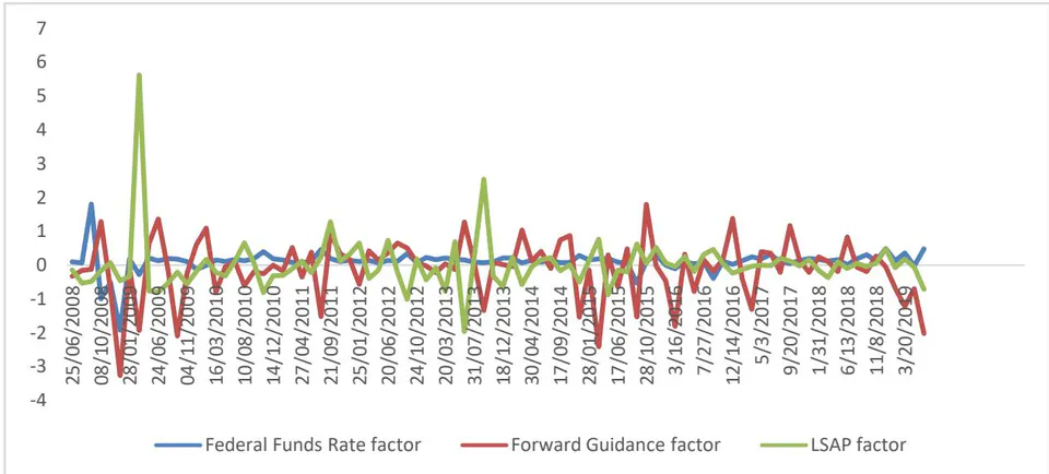
Therefore, we adopt the decomposition method proposed by Swanson, E. T., (2021), focusing on the unexpected UMP shock s of LSAP, forward guidance and federal interest rate:
Firstly, we compile data on the forward guidance and Large-Scale Asset Purchase (LSAP) components for each Federal Open Market Committee (FOMC) announcement, spanning from July 1991 to June 2019. This dataset includes the date of each FOMC announcement and multiple asset price changes observed within the 30-minute window surrounding each announcement. The asset prices tracked encompass federal funds futures (contract interest rate for the current month and contract interest rate for the next six months), Eurodollar futures (contract interest rate for the current quarter and contract interest rate for the next eight quarters), Treasury yields (3 months, 6 months, and 2-, 5-, 10-, and 30-year Treasury bonds), stock markets (S & P 500 index), and exchange rates (JPY/USD and USD/EUR).
Secondly, the response to asset price changes is constructed into a matrix in which is the price response of the j-th asset to the i-th FOMC announcement 30 minutes after the release. This model can be explained by the factor model:
where representing a matrix containing unobserved factors, is a matrix of loadings of asset price responses to factors, and is a matrix of time-uncorrelated white noise residuals. If , then the data can be well described by uncorrelated white noise processes; if , the data can be explained by the linear combination of white noise and one factor, and so on. We find that three-factor model can best explain the model.
Each column under the F matrix has the following four possibilities:
The unexpected portion of changes in the federal funds rate at each FOMC meeting;
Unexpected portions of forward-looking guidance changes;
Unexpected portions of any LSAP announcement;
News related to monetary policy or any other aspect of the economy systematically disclosed in FOMC announcements.
Thirdly, we estimate the F matrix. To estimate the unobservable factors , we first extract the first three principal components of the data . These principal components correspond to the three elements in FOMC announcements that have the largest systematic impact on the assets in in the sample, and together they explain approximately of the variance in .
However, principal components are only statistical decompositions without structural interpretation.
Since a 3x3 orthogonal matrix (U) can be completely determined by three parameters, three assumptions are required to determine the federal funds rate impact, forward guidance impact, and LSAP impact:
- It is assumed that changes in forward guidance have no impact on the current federal funds rate. This definition is adopted by Hanson, S., Stein, J., (2015) .
The decomposition result is presented in figure 5.
It is assumed that large-scale asset purchases have no impact on the current federal funds rate. Since large-scale asset purchases mostly occurred in the era of zero interest rate lower bound, it is more reasonable.
It is assumed that prior to the zero interest rate era, the impact of large-scale asset purchases was small and could be ignored.
b) Empirical Design
In the baseline regression, we aim to prove the inverse correlation between the U. S. bond interest rates and EM bond demand, hence we put forward Hypothesis 1:
Hypothesis 1: Expansionary (contractionary) Federal Reserve's unconventional monetary policy will lead to cross-border bond inflows (outflows) to (from) emerging market countries, indicating an inverse correlation between UMP and EM bond demand.
To verify Hypothesis 1, we perform the baseline regression:
The explained variable, denoted as Flow (bflow in regression), represents the capital flow of emerging market bond markets. The selected emerging market countries for this analysis include Argentina, Bangladesh, Brazil, Chile, China, Colombia, Czech Republic, Egypt, India, Indonesia, Malaysia, Mexico, Nigeria, Pakistan, Peru, Philippines, Romania, Thailand, United Arab Emirates, and Vietnam. The data consist of holdings of various funds in different countries at the micro fund level.
The independent variable represents unanticipated unconventional monetary policy shocks, including three types, LSAP shocks, forward guidance shocks, and federal funds rate shocks. Each shock includes a monthly average shock and a monthly total shock.
For control variables, we refer to traditional pull and push factors (Lakdawala et al., 2021 ; Ahmed et al., 2017 ; Anaya et al., 2017 ; Dahlhaus and Vasishtha, 2020 ; Mishra et al., 2014 ). Global risk preference, US economic we add global-level variables and country-level data as controls. Global variables include U.S. economic policy uncertainty (epu), panic index (vix), federal funds rate (federalrate), U.S. M2 growth (UsM2growth), MSCI global index (MSCiglobal), and crude oil price index return (Crudeoil return); The national level includes MSCI country index (MSCI), each country's debt/GDP (debt_to_GDP), each country's financial development index (FDIndex), each country's money market interest rate (mminterest), each country's capital market openness (ka_open), each country's actual GDP growth rate (gdp_growth). Among them, the fear index is also used as an alternative indicator of global risk appetite. In order to avoid the influence of extreme values in the sample, this paper performs a winnowing process on all continuous variables at the and quantiles. At the same time, all explanatory variables and control variables are lagged first-order in the regression to reduce endogeneity.
In the benchmark regression equation, and represent country fixed effects and year fixed effects respectively. The period of our sample regression is 2008-2019.
In accordance with section 3, two possible mechanisms are that expansionary unconventional monetary policy reduces global risk aversion, thereby leading to capital inflows into the bond markets of emerging countries; Another mechanism also emerges, that is, quantitative easing itself has inertia and sends a signal to the market to continue easing, thus leading to capital inflows into the bond markets of emerging market countries. Therefore, we then set out to examine two mechanisms through which Hypothesis works: risk appetite mechanism and signal mechanism.
Hypothesis 2: One mechanism through which the expansionary (contractionary) Fed's unconventional monetary policy triggers cross-border bond inflows (outflows) in (from) emerging market countries is by reducing (increasing) risk appetite.
Hypothesis 3: One mechanism through which the expansionary (contractionary) Fed's unconventional monetary policy triggers cross-border bond inflows (outflows) in (from) emerging market countries is by sending expansionary (contractionary) signals to the market.
To verify hypothesis 2, the following regression is designed:
In continuation with the baseline regression, we augment the model by incorporating a cross-term of the VIX, which indicates the level of risk tolerance, and the impact of unconventional monetary policy. If both coefficients are significantly positive, it suggests that there is an effect amplifying the impact of monetary policy through VIX. Additionally, control variables, country fixed effects, and year fixed effects are included in the regression model.
To verify Hypothesis 3, the following regression is designed:
So the cross-term is added. The focus of the third hypothesis revolves around examining the presence of "inertia" in unconventional monetary policies. In this context, inertia refers to the tendency for expansionary unconventional monetary policies to elicit expansionary expectations, and for contractionary policies to prompt contractionary expectations. This expectation formation process resembles adaptive expectations. To capture this inertia in unconventional monetary policy shocks, we introduce a variable termed "policy inertia." This variable represents the number of consecutive occurrences of a certain unconventional monetary policy shock being positive or negative. Specifically, if a monetary policy shock is positive for consecutive times, the variable takes the value of ; if it is negative for consecutive times, then the variable takes the value of -m. When the policy changes, the variable takes the value of -1 or 1, depending on whether it changes from easing to tightening or vice versa.
Finally, this section re-examines the asymmetry of unconventional monetary policy mentioned in the theoretical conclusion.
Hypothesis 4: The tightening effect of the tightening Fed's unconventional monetary policy is greater than the easing effect of the expansionary policy.
To verify Hypothesis 3, the following regression is designed:
Since the Federal Reserve proposed the normalization of monetary policy at the end of 2014, heterogeneity testing can be carried out by filtering the year. If the result holds , it means that there is asymmetry in unconventional monetary policy, and the capital outflow caused by tightening is greater than the inflow induced by its expansionary counterpart.
c) Empirical Results
We present the disruptive statistics in Table 1.
| Variable name | Variable label | N | Mean | St.d | Min | Max | Source of data |
| Average LSAP shock | avglsap | 144 | 0.0022128 | 0.7736858 | -1.9618 | 5.6307 | Swanson, E. T. (2021) |
| Average Forward guidance shock | avgfg | 144 | -0.0853297 | 0.850372 | -3.2665 | 1.8037 | Swanson, E. T. (2021) |
| Average Federal fund rate shock | avgfr | 144 | 0.1085892 | 0.3848341 | -2.01195 | 1.812 | Swanson, E. T. (2021) |
| Total LSAP shock | sumlsap | 144 | -0.0081072 | 0.7849363 | -1.9618 | 5.6307 | Swanson, E. T. (2021) |
| Total Forward guidance shock | sumfg | 144 | -0.0683262 | 0.8773866 | -3.2665 | 2.3233 | Swanson, E. T. (2021) |
| Total Federal fund rate shock | sumffr | 144 | 0.0965944 | 0.5640894 | -4.0239 | 2.739 | Swanson, E. T. (2021) |
| Bond capital flow | bflow | 2880 | 114.4692 | 843.9642 | -5061.315 | 10074.7 | EPFR database |
| MSCI Index | MSCI | 2880 | 0.2281572 | 7.558789 | -32.35121 | 44.94297 | MSCIwebsite |
| Debt/GDP | debt_to_GDP | 2880 | 40.54164 | 17.79983 | 4.915989 | 84.77705 | IFS database |
| Financial development Index | FDIndex | 240 | 0.4581421 | 0.1199692 | 0.28 | 0.72 | WIND database |
| Money market interest rate | mminterest | 2822 | 5.67529 | 5.035576 | 0.35 | 38.32 | IFS database |
| Degree of capital liberalization rate | ka_open | 240 | 0.4373011 | 0.2794157 | 0 | 1 | Chin, Ito(2008) |
| Crude oil price index return | Crudeoilreturn | 144 | -0.0008974 | 0.1032573 | -0.2076677 | 0.297144 | WIND database |
| The U.S. economic policy uncertainty | epu | 144 | 144.7473 | 47.01878 | 79 | 284 | Baker etal.,(2016) |
| Fear index | vix | 144 | 20.10817 | 8.726204 | 10.41 | 59.89 | WIND database |
| Federal funds rate | federalrate | 144 | 0.457056 | 0.7141933 | 0.04 | 2.51 | WIND database |
| US M2 growth rate | UsM2growth | 144 | 0.0060592 | 0.0055143 | -0.0072355 | 0.0210649 | WIND database |
| MSCI global index | msciglobal | 144 | 0.0036087 | 0.0410393 | -0.2028842 | 0.1022302 | MSCI website |
| Real GDP growth | gdp_growth | 960 | 0.0330143 | 0.1520237 | -0.0258437 | 1.110521 | IFS database |
The empirical results of Hypothesis 1 testing are presented in Table 2 and Table 3. Table 2 displays the regression results for LSAP shock, while Table 3 presents the results for Forward Guidance shock. The results for Federal Rate shock are showcased in the robustness check section.
In Table 2, each column represents the results of different regressions, with the only difference being the inclusion of control variables. Across all regressions, the LSAP shock consistently demonstrates a significant positive impact on emerging market bond capital inflow. This indicates that unconventional monetary policy in the form of LSAP positively influences cross-border bond capital flows.
Table 3 presents the impact of the monthly average forward guidance on capital flows in emerging market countries during the current period. Regression results (1) through (10) show that the core explanatory variable, forward guidance shock, does not exhibit a significant impact on the dependent variable, bond capital flow. Moreover, the sign of the impact is inconsistent across regressions. Notably, after adding control variables such as the federal funds rate to regressions (9) and (10), the coefficient of the core explanatory variable, L.avgfg, becomes positive. However, the increase in the t-value does not reach the significance level. Comparing regression (1) with regression (10) reveals that the insignificance in regression (10) is not influenced by collinearity with the federal funds rate.
| VARIABLES | (1) bflow | (2) bflow | (3) bflow | (4) bflow | (5) bflow | (6) bflow | (7) bflow | (8) bflow | (9) bflow | (10) bflow |
| L.avglsap | 177.3** | 166.7** | 149.7** | 147.7** | 222.6** | 233.4** | 227.2** | 203.6** | 393.0** | 430.6** |
| * | * | * | * | * | * | * | * | * | * | |
| (58.83) | (58.79) | (56.52) | (56.27) | (72.14) | (74.11) | (76.49) | (76.19) | (137.1) | (152.8) | |
| L.mminterest_ | -13.27 | -5.014 | 0.165 | 6.673 | 6.187 | 3.819 | 5.210 | 8.332 | 10.72 | |
| (14.99) | (20.23) | (20.43) | (22.26) | (22.39) | (21.93) | (21.77) | (26.29) | (25.78) | ||
| L.debt_to_GDP_ | -2.510 | -4.055 | -4.534 | -3.801 | -3.627 | -3.582 | -4.259 | -4.571 | ||
| (4.788) | (4.999) | (5.448) | (4.947) | (5.016) | (5.002) | (5.861) | (5.834) | |||
| L.FDIndex_ | 1,425* | 1,624* | 1,804** | 1,767** | 1,781** | 1,983** | 2,031** | |||
| (770.9) | (854.4) | (784.7) | (795.0) | (792.1) | (963.5) | (969.8) | ||||
| L.vix | -6.715 | -4.388 | -3.331 | -7.195 | 31.91** | 28.84** | ||||
| (5.559) | (5.763) | (5.357) | (6.074) | (14.74) | (14.19) | |||||
| L.kaopen | 41.27 | 36.95 | 34.84 | 49.41 | 45.08 | |||||
| (130.3) | (131.2) | (130.3) | (150.9) | (145.9) | ||||||
| L.gdp_growth | 195.7 | 194.5 | 238.7 | 169.4 | 139.1 | |||||
| (234.2) | (236.6) | (235.7) | (268.1) | (277.4) | ||||||
| L.MSCI_ | 3.080 | 5.893 | 3.217 | 3.788 | ||||||
| (5.530) | (5.496) | (7.817) | (7.639) | |||||||
| L.msciglobal | -2,411* | -2,072 | -1,421 | |||||||
| (1,398) | (1,978) | (1,855) | ||||||||
| L.federalrate | 170.1 | 23.20 | ||||||||
| (172.6) | (153.2) | |||||||||
| L.Crudeoilreturn | -347.2 | -293.2 | ||||||||
| (717.0) | (725.2) | |||||||||
| L.epu | - | - | ||||||||
| 7.799** | 7.239** | |||||||||
| (3.202) | (2.988) | |||||||||
| L.USM2growth | -37,224 | |||||||||
| (36,955) | ||||||||||
| Country Fixed Effect | Y | Y | Y | Y | Y | Y | Y | Y | Y | Y |
| Year Fixed Effect | Y | Y | Y | Y | Y | Y | Y | Y | Y | Y |
| Observations | 2822 | 2822 | 2822 | 2822 | 2822 | 2822 | 2822 | 2822 | 2822 | 2822 |
| R-squared | 0.122 | 0.128 | 0.134 | 0.140 | 0.153 | 0.157 | 0.158 | 0.163 | 0.230 | 0.241 |
| VARIABLES | (1) bflow | (2) bflow | (3) bflow | (4) bflow | (5) bflow | (6) bflow | (7) bflow | (8) bflow | (9) bflow | (10) bflow |
| L.avfgf | -19.88 | -16.01 | -23.27 | -21.08 | -19.32 | -19.82 | -17.41 | -11.92 | 79.87 | 44.83 |
| (53.42) | (53.60) | (45.31) | (45.55) | (56.58) | (56.96) | (55.86) | (56.60) | (106.2) | (76.79) | |
| L.mminterest_ | -13.00 | -4.750 | 0.469 | 6.830 | 6.483 | 2.895 | 4.916 | 11.42 | 12.11 | |
| (15.17) | (20.52) | (20.76) | (22.64) | (22.80) | (22.29) | (22.05) | (26.17) | (26.06) | ||
| L.debt_to_GDP_ | -2.523 | -4.075 | -4.559 | -3.929 | -3.661 | -3.604 | -4.622 | -4.720 | ||
| (4.812) | (5.031) | (5.498) | (4.982) | (5.055) | (5.044) | (5.899) | (5.910) | |||
| L.FDIndex_ | 1,430* | 1,626* | 1,775** | 1,721** | 1,746** | 1,950** | 1,966** | |||
| (768.8) | (849.7) | (779.5) | (787.0) | (786.9) | (946.1) | (944.9) | ||||
| L.vix | -3.579 | -1.232 | 0.181 | -5.483 | 6.964 | 8.826 | ||||
| (6.065) | (6.144) | (6.177) | (6.905) | (16.22) | (14.65) | |||||
| L.kaopen | 37.77 | 31.30 | 29.28 | 44.63 | 42.25 | |||||
| (132.8) | (133.3) | (132.1) | (153.3) | (151.6) | ||||||
| L.gdp_growth | 177.2 | 176.4 | 237.1 | 136.8 | 116.8 | |||||
| (245.7) | (249.2) | (246.3) | (274.7) | (283.2) | ||||||
| L.MSCI_ | 4.711 | 8.183 | 5.784 | 6.132 | ||||||
| (5.244) | (5.187) | (7.538) | (7.564) | |||||||
| L.msciglobal | - | -3,293 | -2,730 | |||||||
| 3,149** | ||||||||||
| (1,461) | (2,385) | (2,201) | ||||||||
| L.federalrate | 445.4* | 345.9* | ||||||||
| (261.5) | (201.4) | |||||||||
| L.Crudeoilreturn | -611.3 | -590.8 | ||||||||
| (715.5) | (719.5) | |||||||||
| L.epu | -3.764 | -3.420 | ||||||||
| (2.462) | (2.434) | |||||||||
| L.UsM2growth | -19,458 | |||||||||
| (30,251) | ||||||||||
| Country Fixed Effect | Y | Y | Y | Y | Y | Y | Y | Y | Y | Y |
| Year Fixed Effect | Y | Y | Y | Y | Y | Y | Y | Y | Y | Y |
| Constant | -148.3 | 147.8 | 229.9 | -491.0 | -584.6 | -713.7 | -719.9 | -617.6 | -1,484* | -1,250 |
| (127.8) | (269.7) | (434.9) | (529.4) | (610.2) | (624.1) | (620.1) | (616.4) | (767.6) | (800.3) | |
| Observations | 2822 | 2822 | 2822 | 2822 | 2822 | 2822 | 2822 | 2822 | 2822 | 2822 |
| R-squared | 0.113 | 0.120 | 0.122 | 0.127 | 0.135 | 0.136 | 0.139 | 0.148 | 0.206 | 0.208 |
Table 4 presents the regression results for testing Hypothesis 2. The first four columns focus on the risk-appetite mechanism test of unconventional monetary policy, specifically large-scale asset purchases. Columns (5) to (8) serve as the control group, where (5) and (7) represent mechanism tests of forward guidance, while (6) and (8) are mechanism tests of the federal funds rate.
Upon comparison of regressions (1), (5), and (7), it is evident that in the absence of additional control variables, only the impact of large-scale asset purchases exhibits a moderating effect on the risk- appetite mechanism. The coefficient of the cross-product term is positive and highly significant, whereas the other two monetary policy indicators show no significant impact, thus failing to demonstrate the existence of the mechanism.
Further comparison across regressions (1) to (4) reveals that even after incorporating different control variables, the coefficient of the cross-term remains significantly positive. This indicates that the Federal Reserve's LSAP lead to capital flows into emerging market countries by boosting risk appetite, thereby confirming Hypothesis 2.
| VARIABLES | (1) bflow | (2) bflow | (3) bflow | (4) bflow | (5) bflow | (6) bflow | (7) bflow | (8) bflow |
| L.avglsap | 272.7*** | 252.1*** | 188.5** | 395.7*** | ||||
| (78.92) | (83.91) | (84.79) | (134.5) | |||||
| L.avfgf | -32.96 | 54.78 | ||||||
| (65.48) | (107.9) | |||||||
| L.avgfr | -188.3 | -441.8 | ||||||
| (301.2) | (386.8) | |||||||
| L.avglapsvix | 0.755** | 3.953** | 3.444** | 3.674** | ||||
| (0.351) | (1.618) | (1.485) | (1.833) | |||||
| L.avgfgvix | 0.636 | 3.234* | ||||||
| (0.420) | (1.787) | |||||||
| L.avgffrxvix | 0.128 | 3.186 |
| (0.450) | (1.969) | ||||||
| L.mminterest_ | 4.833 | 2.212 | 8.320 | 10.96 | 12.95 | ||
| (22.04) | (21.95) | (26.16) | (26.28) | (26.91) | |||
| L.debt_to_GDP_ | -3.964 | -3.883 | -4.583 | -4.856 | -4.931 | ||
| (4.992) | (4.942) | (5.840) | (5.898) | (5.921) | |||
| L.FDIndex_ | 1,730** | 1,711** | 1,911** | 1,882** | 1,888** | ||
| (795.7) | (814.9) | (965.8) | (949.6) | (945.5) | |||
| L.vix | -36.73** | -31.02** | 0.434 | -17.81 | -16.82 | ||
| (16.28) | (14.78) | (19.48) | (20.48) | (18.34) | |||
| L.kaopen | 30.60 | 24.02 | 48.45 | 43.83 | 50.77 | ||
| (128.0) | (125.1) | (149.9) | (152.9) | (150.7) | |||
| L.gdp_growth | 174.0 | 181.7 | 126.9 | 97.58 | 135.5 | ||
| (238.8) | (239.9) | (276.3) | (278.9) | (268.4) | |||
| L.MSCI_ | 2.607 | 4.294 | -0.422 | 2.545 | 0.520 | ||
| (6.290) | (6.180) | (8.132) | (7.768) | (8.647) | |||
| L.msciglobal | -5,231** | -5,464** | -4,296* | -5,073* | -6,151** | ||
| (2,234) | (2,274) | (2,530) | (2,672) | (2,722) | |||
| L.federalrate | 360.8** | 112.7 | 372.6 | 319.0* | |||
| (169.6) | (163.9) | (264.4) | (181.2) | ||||
| L.Crudeoilreturn | -565.7 | -801.7 | -837.4 | ||||
| (758.8) | (772.4) | (751.0) | |||||
| L.epu | -7.378** | -3.467 | -3.936* | ||||
| (3.050) | (2.408) | (2.371) | |||||
| Country Fixed Effect | Y | Y | Y | Y | Y | Y | Y |
| Year Fixed Effect | Y | Y | Y | Y | Y | Y | Y |
| Constant | -174.3 | -71.39 | -841.9 | -268.7 | -158.8 | -116.6 | -904.1 |
| (140.5) | (692.1) | (648.1) | (830.8) | (144.5) | (162.7) | (838.8) | |
| Observations | 2822 | 2822 | 2822 | 2822 | 2822 | 2822 | 2822 |
| R-squared | 0.133 | 0.182 | 0.195 | 0.241 | 0.119 | 0.120 | 0.214 |
Table 5 displays the regression results for testing Hypothesis 3. Regressions (1) to (5) examine the mechanism of unconventional monetary policy, specifically large-scale asset purchases. On the other hand, regressions (6) and (8) investigate the inertia mechanism of forward guidance, while regressions (7) and (9) test the inertia mechanism of conventional monetary policy.
Upon examining the inertia mechanism of policy, it becomes apparent that the same holds true solely for large-scale asset purchases. Notably, Hypothesis 3 is confirmed, suggesting that only large-scale asset purchases exhibit the inertia mechanism.
| VARIABLES | (1) | (2) | (3) | (4) | (5) | (6) | (7) | (8) | (9) |
| bflow | bflow | bflow | bflow | bflow | bflow | bflow | bflow | bflow | |
| avglsap | 356.3*** | 392.9*** | 351.5*** | 272.1*** | 296.2** | ||||
| (91.81) | (107.5) | (100.0) | (93.89) | (123.6) | |||||
| avgfg | -6.777 | 153.0 | |||||||
| (56.38) | (115.4) | ||||||||
| avgfrr | -81.86 | -559.3 | |||||||
| (270.4) | (370.0) | ||||||||
| L.avglxlsapcon | 85.02** | 96.70** | 135.1*** | 151.3*** | 167.0*** | ||||
| (39.07) | (42.55) | (49.48) | (52.73) | (54.17) | |||||
| L.avgfgxfgcon | 103.0** | 231.0*** | |||||||
| (42.69) | (70.25) | ||||||||
| L.avgfrxffrcn | 99.80** | 204.3*** | |||||||
| (48.07) | (58.11) | ||||||||
| L.mminterest_ | -6.493 | 1.343 | 3.020 | 0.267 | 7.020 | -5.526 | -5.184 | 10.38 | 11.65 |
| (21.86) | (22.59) | (22.26) | (22.16) | (26.76) | (22.53) | (23.09) | (26.93) | (27.11) | |
| debt_to_GDP_ | -2.663 | -3.795 | -3.780 | -3.774 | -4.765 | -2.744 | -2.757 | -5.410 | -5.260 |
| (5.087) | (4.870) | (4.802) | (4.759) | (5.795) | (5.176) | (5.166) | (5.803) | (5.870) | |
| FDIndex_ | 1,842** | 1,848** | 1,799** | 1,890** | 1,853** | 1,856** | |||
| (812.9) | (796.6) | (805.8) | (931.0) | (930.6) | (911.5) | ||||
| L.vix | 11.49 | 14.21 | 5.095 | 2.401 | 13.63 | 4.199 | 3.373 | -21.95 | -8.791 |
| (9.623) | (9.572) | (9.207) | (9.124) | (15.16) | (8.069) | (8.539) | (21.26) | (13.94) | |
| L.kaopen | 38.75 | 35.41 | 28.62 | 46.25 | 41.56 | 50.93 | |||
| (126.1) | (124.7) | (122.2) | (149.2) | (147.4) | (148.0) | ||||
| gdp_growth | 125.9 | 183.4 | 177.7 | 83.20 | 35.18 | 89.33 | |||
| (239.2) | (238.8) | (242.6) | (282.9) | (293.5) | (275.3) | ||||
| L.MSCI_ | -4.785 | -1.319 | -0.0789 | -3.465 | -4.133 | -5.759 | |||
| (6.309) | (6.023) | (5.942) | (8.408) | (8.918) | (9.498) | ||||
| L.msciglobal | -4,341** | -5,038*** | -3,755* | -5,935** | -6,485** |
L.federalrate L.Crudeoilreturn L.epu Country Fixed Effect Year Fixed Effect Constant Observations R-squared
| (1,727) | (1,909) | (2,232) | (2,845) | (2,744) | ||||
| L.federalrate | 342.4** | 215.1 | 507.7* | 361.3** | ||||
| (157.6) | (164.1) | (260.7) | (180.8) | |||||
| L.Crudeoilreturn | -616.8 | -908.4 | -912.4 | |||||
| (730.9) | (728.2) | (709.0) | ||||||
| L.epu | -5.142*** | -5.851*** | -6.211*** | -5.634*** | -8.297** | -3.329** | -3.217** | -5.443** |
| (1.584) | (1.924) | (1.938) | (1.778) | (3.234) | (1.359) | (1.516) | (2.598) | |
| Country Fixed Effect | Y | Y | Y | Y | Y | Y | Y | Y |
| Year Fixed Effect | Y | Y | Y | Y | Y | Y | Y | Y |
| Constant | 582.6 | -329.9 | -92.56 | -728.5 | -521.9 | 520.0 | 534.4 | -793.1 |
| (507.3) | (651.7) | (649.3) | (631.3) | (761.5) | (517.3) | (494.3) | (738.2) | |
| Observations | 2822 | 2822 | 2822 | 2822 | 2822 | 2822 | 2822 | 2822 |
| R-squared | 0.203 | 0.218 | 0.234 | 0.245 | 0.257 | 0.163 | 0.164 | 0.257 |
Tables 6 and 7 present the regression results for testing Hypothesis 4. In Table 6, the impact of U.S. unconventional monetary policy shocks on cross-border bond capital flows in emerging market countries from 2008 to 2013 is examined. Columns (1) and (4) analyze the impact of large-scale asset purchases on cross-border capital flows of bonds, while (2) and (5) investigate the impacts of forward guidance. Lastly, columns (3) and (6) assess the impact of federal funds rate shocks on bond cross-border capital flows. It is observed that during the quantitative easing cycle, large-scale asset purchases have a significant impact on cross-border inflows of bonds from emerging market countries.
| VARIABLES | (1) bflow | (2) bflow | (3) bflow | (4) bflow | (5) bflow | (6) bflow |
| avglsap | 757.1*** | 547.9** | ||||
| (281.4) | (233.8) | |||||
| avgfg | -80.3 | -85.26 | ||||
| (61.23) | (62.01) | |||||
| avgffr | -89.92 | -68.80 | ||||
| (77.15) | (76.61) | |||||
| L.mminterest_ | 42.16 | 34.97 | 34.56 | 34.93 | 28.50 | 28.04 |
| (29.35) | (28.48) | (29.55) | (27.38) | (26.40) | (26.55) | |
| debt_to_GDP_ | -8.904 | -8.136 | -8.122 | -8.775 | -8.206 | -8.251 |
| (6.023) | (6.333) | (6.492) | (5.743) | (5.975) | (6.027) | |
| FDIndex_ | 3,046* | 2,917 | 2,984 | 3,114** | 3,048* | 3,097* |
| (1,623) | (1,759) | (1,806) | (1,556) | (1,646) | (1,633) | |
| L.vix | 113.8** | 30.99** | 2.608 | 114.5*** | 54.72*** | 42.44* |
| (44.59) | (12.37) | (18.44) | (43.00) | (17.17) | (24.03) | |
| L.kaopen | 119.2 | 104.7 | 103.1 | 128.9 | 120.2 | 121.7 |
| (101.7) | (115.4) | (117.1) | (97.16) | (102.0) | (101.8) | |
| gdp_growth | 180.0 | 35.74 | 96.50 | 161.6 | 74.22 | 102.0 |
| (136.7) | (161.1) | (159.9) | (154.9) | (124.8) | (119.7) | |
| L.MSCI_ | -7.775 | 3.992 | 5.840 | -13.33 | -6.141 | -6.187 |
| (8.966) | (6.862) | (7.623) | (9.398) | (8.296) | (8.484) | |
| L.msciglobal | 7,653*** | 2,750 | -272.6 | 8,050*** | 4,340*** | 3,007** |
| (2,344) | (1,731) | (1,229) | (2,139) | (1,531) | (1,404) | |
| L.federalrate | -676.6*** | -318.4** | -0.0811 | -513.7*** | -194.6 | -21.77 |
| (233.9) | (125.7) | (73.54) | (191.2) | (118.5) | (101.4) | |
| L.Crudeoilreturn | -2,870*** | -887.2* | -674.5 | -3,268*** | -2,024** | -1,940** |
| (1,049) | (474.0) | (594.1) | (1,004) | (793.7) | (886.0) | |
| L.epu | -22.49** | -2.804 | -1.297 | -21.13** | -7.527** | -7.011* |
| (8.689) | (2.475) | (3.245) | (8.152) | (3.444) | (3.923) | |
| UsM2growth | 84,035*** | 97,965*** | 109,789*** | |||
| (22,339) | (34,993) | (32,464) | ||||
| Country Fixed Effect | Y | Y | Y | Y | Y | Y |
| Year Fixed Effect | Y | Y | Y | Y | Y | Y |
| Constant | 195.3 | -1,092 | -1,410 | -754.1 | -1,822* | -2,087** |
| (863.9) | (953.9) | (1,042) | (800.8) | (1,007) | (988.0) | |
| Observations | 1411 | 1411 | 1411 | 1411 | 1411 | 1411 |
| R-squared | 0.348 | 0.291 | 0.249 | 0.406 | 0.367 | 0.361 |
Through comparison, it is evident that the impact of the initial large-scale asset purchase on capital flows was consistently positive and significant both before and after 2014. However, the coefficient became significantly larger after 2014, indicating that capital outflows during contractionary periods are more pronounced than inflows during expansionary periods. This suggests that the impact of unconventional monetary policies on cross-border capital flows is asymmetric. Additionally, the significance of the impact
of large-scale asset purchases on cross-border capital flows has decreased, while the significance of the impact of the federal funds rate has increased. This implies that traditional monetary policy has diminished in significance post-2014, with a larger post-action space compared to before 2014.
Overall, these findings confirm Hypothesis 4 regarding the asymmetric impact of unconventional monetary policies and the changing significance of traditional monetary policy.
| VARIABLES | (1) bflow | (2) bflow | (3) bflow | (4) bflow | (5) bflow | (6) bflow |
| avglsap | 2,010** | 2,552* | ||||
| (783.5) | (1,425) | |||||
| avgfr | -1,291 | -1,452* | ||||
| (3,565) | (810.8) | |||||
| avgfg | -100.9 | 706.1* | ||||
| (278.5) | (394.2) | |||||
| L.mminterest_ | 46.13 | 27.90 | 27.90 | 85.26 | 85.26 | 85.26 |
| (82.90) | (88.17) | (88.17) | (76.82) | (76.82) | (76.82) | |
| debt_to_GDP_ | -19.30 | -30.30 | -30.30 | -0.0250 | -0.0250 | -0.0250 |
| (34.56) | (34.23) | (34.23) | (20.38) | (20.38) | (20.38) | |
| FDIndex_ | 6,446 | 6,842 | 6,842 | 3,854 | 3,854 | 3,854 |
| (4,721) | (4,565) | (4,565) | (3,223) | (3,223) | (3,223) | |
| L.vix | 79.79* | -104.8 | 34.95 | 14.37 | -361.7** | -89.12* |
| (42.52) | (133.6) | (419.4) | (68.08) | (171.5) | (51.59) | |
| L.kaopen | -527.0 | -523.6 | -523.6 | -444.2 | -444.2 | -444.2 |
| (496.1) | (521.1) | (521.1) | (473.4) | (473.4) | (473.4) | |
| gdp_growth | -92.25 | -771.0 | -771.0 | 75.88 | 75.88 | 75.88 |
| (1,191) | (1,262) | (1,262) | (1,217) | (1,217) | (1,217) | |
| L.MSCI_ | 20.94 | 4.335 | 4.335 | 4.430 | 4.430 | 4.430 |
| (20.80) | (21.05) | (21.05) | (19.76) | (19.76) | (19.76) | |
| L.msciglobal | -12,682* | -32,354 | 6,484 | -14,023 | -56,243*** | -25,537*** |
| (6,620) | (30,006) | (101,031) | (9,775) | (20,781) | (8,779) | |
| L.federalrate | 639.9** | 301.0 | 4,072 | 911.1* | 233.4 | 244.6 |
| (268.0) | (3,064) | (9,552) | (506.5) | (191.5) | (194.9) | |
| L.Crudeoilreturn | -650.0 | 3,899 | -847.5 | -955.0 | 6,285** | 2,929* |
| (1,451) | (3,459) | (12,427) | (2,688) | (2,395) | (1,537) | |
| L.epu | -7.042** | -7.302 | 0.521 | -9.741** | -11.29** | -8.030** |
| (2.837) | (7.718) | (19.63) | (4.055) | (4.541) | (3.681) | |
| UsM2growth | 73,831 | -55,562 | -112,491** | |||
| (115,314) | (59,762) | (50,975) | ||||
| Country Fixed Effect | Y | Y | Y | Y | Y | Y |
| Year Fixed Effect | Y | Y | Y | Y | Y | Y |
| Constant | -4,320* | -553.1 | -3,706 | -3,784 | 2,908 | -656.3 |
| (2,538) | (4,019) | (9,439) | (2,274) | (3,539) | (2,265) | |
| Observations | 1411 | 1411 | 1411 | 1411 | 1411 | 1411 |
| R-squared | 0.293 | 0.375 | 0.375 | 0.386 | 0.386 | 0.386 |
V. ROBUSTNESS CHECK
In this section, we conduct two types of robustness checks. First, we establish a placebo group by substituting the explanatory variable with a conventional monetary policy variable (i.e., federal funds rate shock). Second, we utilize the sum of monthly overall monetary policy shocks as the independent variable instead of the monthly average monetary policy shock.
a) Robustness Check for H1
We first present the robustness check result of Hypothesis 1, in which we present the regression result of conventional monetary policy (i.e. federal fund rate shock) on capital flow, and that of alternative unconventional monetary policy indicators on capital flow, as shown in Table 8.
| VARIABLES | (1) bflow | (2) bflow | (3) bflow | (4) bflow | (5) bflow | (6) bflow | (7) bflow | (8) bflow | (9) bflow | (10) bflow |
| L.avgfr | -41.01 | -38.01 | -54.95 | -53.92 | -282.0 | -256.3 | -218.7 | -538.3 | -501.7 | -497.7 |
| (51.80) | (51.95) | (46.00) | (46.68) | (217.1) | (220.6) | (271.7) | (342.6) | (368.4) | (368.1) | |
| L.mminterest_ | -13.03 | -4.682 | 0.509 | 7.254 | 6.870 | 4.691 | 9.790 | 13.36 | 15.13 | |
| (15.04) | (20.61) | (20.84) | (22.78) | (22.96) | (22.88) | (22.48) | (26.71) | (26.24) | ||
| L.debt_to_GDP_ | -2.545 | -4.094 | -4.587 | -3.995 | -3.827 | -3.909 | -4.675 | -4.906 | ||
| (4.805) | (5.020) | (5.492) | (4.977) | (5.061) | (5.033) | (5.925) | (5.917) | |||
| L.FDIndex_ | 1,429* | 1,631* | 1,780** | 1,747** | 1,818** | 1,952** | 1,983** | |||
| (769.9) | (851.8) | (780.9) | (793.9) | (796.0) | (940.7) | (943.5) | ||||
| L.vix | -5.208 | -2.853 | -1.831 | -12.59** | 9.747 | 6.594 | ||||
| (5.004) | (5.159) | (4.746) | (5.561) | (13.04) | (13.53) | |||||
| L.kaopen | 37.18 | 33.36 | 33.36 | 52.55 | 49.11 | |||||
| (132.0) | (132.1) | (130.0) | (151.5) | (148.0) | ||||||
| L.gdp_growth | 172.0 | 172.5 | 261.4 | 178.0 | 153.7 | |||||
| (245.9) | (248.6) | (233.2) | (260.6) | (271.2) | ||||||
| L.MSCI_ | 2.844 | 5.671 | 3.396 | 3.981 | ||||||
| (6.694) | (6.118) | (8.392) | (8.299) | |||||||
| L.msciglobal | -5,217*** | -4,423* | -3,992* | |||||||
| (1,998) | (2,500) | (2,374) | ||||||||
| L.federalrate | 367.1* | 276.8* | ||||||||
| (189.4) | (142.1) | |||||||||
| L.Crudeoilreturn | -652.7 | -631.2 | ||||||||
| (699.8) | (705.6) | |||||||||
| L.epu | -4.358* | -3.707 | ||||||||
| (2.484) | (2.346) | |||||||||
| L.UsM2growth | -26,345 | |||||||||
| (35,730) | ||||||||||
| Country Fixed Effect | Y | Y | Y | Y | Y | Y | Y | Y | Y | |
| Year Fixed Effect | Y | Y | Y | Y | Y | Y | Y | Y | Y | |
| Constant | -137.1 | 158.7 | 245.3 | -475.5 | -510.3 | -644.4 | -657.8 | -409.9 | -1,188 | |
| (126.7) | (263.6) | (431.7) | (529.2) | (602.1) | (612.9) | (614.7) | (608.8) | (741.7) | ||
| Observations | 2822 | 2822 | 2822 | 2822 | 2822 | 2822 | 2822 | 2822 | 2822 | |
| R-squared | 0.113 | 0.120 | 0.122 | 0.128 | 0.140 | 0.141 | 0.141 | 0.162 | 0.212 |
| VARIABLES | (1) bflow | (2) bflow | (3) bflow | (4) bflow | (5) bflow | (6) bflow | (7) bflow | (8) bflow | (9) bflow | (10) bflow |
| L-sumlsap | 178.9*** | 168.3*** | 151.0*** | 149.0*** | 224.2*** | 234.5*** | 228.2*** | 204.8*** | 393.0*** | 430.6*** |
| (58.90) | (58.86) | (56.60) | (56.35) | (72.34) | (74.29) | (76.72) | (76.42) | (137.1) | (152.8) | |
| L.mminterest_ | -13.26 | -4.999 | 0.180 | 6.682 | 6.209 | 3.857 | 5.245 | 8.332 | 10.72 |
| VARIABLES | (1) bflow | (2) bflow | (3) bflow | (4) bflow | (5) bflow | (6) bflow | (7) bflow | (8) bflow | (9) bflow | (10) bflow |
| L-sumlsap | 178.9*** | 168.3*** | 151.0*** | 149.0*** | 224.2*** | 234.5*** | 228.2*** | 204.8*** | 393.0*** | 430.6*** |
| (58.90) | (58.86) | (56.60) | (56.35) | (72.34) | (74.29) | (76.72) | (76.42) | (137.1) | (152.8) | |
| L.mminterest_ | -13.26 | -4.999 | 0.180 | 6.682 | 6.209 | 3.857 | 5.245 | 8.332 | 10.72 |
L.debt_to_GDP_
| (14.99) | (20.23) | (20.43) | (22.26) | (22.39) | (21.93) | (21.76) | (26.29) | (25.78) | |
| L.debt_to_GDP_ | -2.510 | -4.055 | -4.534 | -3.804 | -3.631 | -3.586 | -4.259 | -4.571 | |
| (4.788) | (4.999) | (5.449) | (4.947) | (5.016) | (5.002) | (5.861) | (5.834) | ||
| L.FDIndex_ | 1,426* | 1,624* | 1,805** | 1,769** | 1,782** | 1,983** | 2,031** | ||
| (770.8) | (854.2) | (784.6) | (794.9) | (792.0) | (963.5) | (969.8) | |||
| L.vix | -6.633 | -4.308 | -3.261 | -7.134 | 31.91** | 28.84** | |||
| (5.563) | (5.766) | (5.359) | (6.075) | (14.74) | (14.19) | ||||
| L.kaopen | 41.14 | 36.86 | 34.76 | 49.41 | 45.08 | ||||
| (130.3) | (131.2) | (130.3) | (150.9) | (145.9) | |||||
| L.gdp_growth | 195.2 | 194.0 | 238.3 | 169.4 | 139.1 | ||||
| (234.1) | (236.5) | (235.6) | (268.1) | (277.4) | |||||
| L.MSCI_ | 3.057 | 5.871 | 3.217 | 3.788 | |||||
| (5.532) | (5.499) | (7.817) | (7.639) | ||||||
| L.msciglobal | -2,410* | -2,072 | -1,421 | ||||||
| (1,398) | (1,978) | (1,855) | |||||||
| L.federalrate | 170.1 | 23.20 | |||||||
| (172.6) | (153.2) | ||||||||
| L.Crudeoilreturn | -347.2 | -293.2 | |||||||
| (717.0) | (725.2) | ||||||||
| L.epu | -7,799** | -7,239** | |||||||
| (3.202) | (2.988) | ||||||||
| L.USM2growth | -37,224 | ||||||||
| (36,955) | |||||||||
| Country Fixed Effect | Y | Y | Y | Y | Y | Y | Y | Y | Y |
| Year Fixed Effect | Y | Y | Y | Y | Y | Y | Y | Y | Y |
| Constant | -158.6 | 143.0 | 224.7 | -493.9 | -556.7 | -711.5 | -716.0 | -638.9 | -917.7 |
| (124.4) | (269.0) | (429.1) | (526.5) | (603.7) | (616.5) | (614.8) | (611.1) | (756.1) | |
| Observations | 2822 | 2822 | 2822 | 2822 | 2822 | 2822 | 2822 | 2822 | 2822 |
| R-squared | 0.122 | 0.128 | 0.135 | 0.140 | 0.154 | 0.157 | 0.158 | 0.164 | 0.230 |
L.FDIndex_
| VARIABLES | (1) | (2) | (3) | (4) | (5) | (6) | (7) | (8) | (9) | (10) |
| bflow | bflow | bflow | bflow | bflow | bflow | bflow | bflow | bflow | bflow | |
| L,sumfg | -23.03 | -19.19 | -25.55 | -23.43 | -22.25 | -21.42 | -18.83 | -13.71 | 79.87 | 44.83 |
| (53.00) | (53.15) | (44.97) | (45.22) | (56.73) | (57.06) | (55.89) | (56.55) | (106.2) | (76.79) | |
| L.mminterest_ | -13.00 | -4.757 | 0.459 | 6.752 | 6.451 | 2.879 | 4.885 | 11.42 | 12.11 | |
| (15.16) | (20.53) | (20.78) | (22.64) | (22.80) | (22.29) | (22.05) | (26.17) | (26.06) | ||
| L.debt_to_GDP_ | -2.520 | -4.072 | -4.553 | -3.928 | -3.661 | -3.603 | -4.622 | -4.720 | ||
| (4.812) | (5.031) | (5.499) | (4.981) | (5.054) | (5.043) | (5.899) | (5.910) | |||
| L.FDIndex_ | 1,430* | 1,625* | 1,776** | 1,721** | 1,746** | 1,950** | 1,966** | |||
| (768.4) | (849.3) | (779.2) | (786.6) | (786.4) | (946.1) | (944.9) | ||||
| L.vix | -3.370 | -1.100 | 0.292 | -5.365 | 6.964 | 8.826 | ||||
| (6.146) | (6.223) | (6.267) | (6.991) | (16.22) | (14.65) | |||||
| L.kaopen | 37.69 | 31.25 | 29.25 | 44.63 | 42.25 | |||||
| (132.9) | (133.4) | (132.2) | (153.3) | (151.6) | ||||||
| L.gdp_growth | 176.5 | 175.8 | 236.5 | 136.8 | 116.8 | |||||
| (245.6) | (249.1) | (246.3) | (274.7) | (283.2) | ||||||
| L.MSCI_ | 4.695 | 8.165 | 5.784 | 6.132 | ||||||
| (5.235) | (5.183) | (7.538) | (7.564) | |||||||
| L.msciglobal | -3,147** | -3,293 | -2,730 | |||||||
| (1,458) | (2,385) | (2,201) | ||||||||
| L.federalrate | 445.4* | 345.9* | ||||||||
| (261.5) | (201.4) | |||||||||
| L.Crudeoilreturn | -611.3 | -590.8 | ||||||||
| (715.5) | (719.5) | |||||||||
| L.epu | -3.764 | -3.420 | ||||||||
| (2.462) | (2.434) | |||||||||
| L.UsM2growth | -19,458 | |||||||||
| (30,251) | ||||||||||
| Country Fixed Effect | Y | Y | Y | Y | Y | Y | Y | Y | Y | Y |
| Year Fixed Effect | Y | Y | Y | Y | Y | Y | Y | Y | Y | Y |
| Constant | -148.8 | 147.4 | 229.5 | -491.5 | -586.9 | -715.6 | -721.6 | -619.1 | -1,484* | -1,250 |
| (127.8) | (269.7) | (435.1) | (529.3) | (610.4) | (624.7) | (620.6) | (616.9) | (767.6) | (800.3) | |
| Observations | 2822 | 2822 | 2822 | 2822 | 2822 | 2822 | 2822 | 2822 | 2822 | 2822 |
| R-squared | 0.113 | 0.120 | 0.122 | 0.127 | 0.135 | 0.137 | 0.139 | 0.148 | 0.206 | 0.208 |
It's apparent that although there's a negative correlation between the previous period's federal funds rate impact and the current period's cross-border capital flow of bonds, this relationship lacks significance. This can be attributed to the near-zero interest rates persisting for nearly 7 years from 2008 to 2019. Consequently, despite brief interest rate hikes by the Federal Reserve post-2015, overall monetary expansion primarily relied on unconventional monetary policies. Nonetheless, traditional monetary policy still holds some influence after 2015, as evidenced by the negative sum of coefficients for L.avgfr and L.federalrate in (9) and (10).
From the preceding results, it's evident that the primary avenue through which the Fed's unconventional monetary policy impacts bond capital flows in emerging markets is via large-scale asset purchases, i.e., quantitative easing. Forward guidance exhibits limited impact on cross-border bond capital flows, while the rise in the federal funds rate notably curtails such flows. However, its effect remains insignificant due to the constraints posed by the zero interest rate era. Thus, Hypothesis 1 is validated.
b) Robustness check for H2 and H3
The robustness check results presented in Table 11 and 12 demonstrate consistent findings, affirming the robustness of our analysis
| VARIABLES | (1) bflow | (2) bflow | (3) bflow | (4) bflow | (5) bflow | (6) bflow | (7) bflow | (8) bflow |
| L-sumlsap | 275.2*** | 252.2*** | 188.2** | 395.7*** | ||||
| (79.06) | (83.89) | (84.94) | (134.5) | |||||
| L-sumfg | -36.77 | 54.78 | ||||||
| (64.92) | (107.9) | |||||||
| L-sumffr | 110.5 | -96.48 | ||||||
| (145.0) | (244.0) | |||||||
| L-sumlsapxvix | 0.756** | 3.936** | 3.432** | 3.674** | ||||
| (0.351) | (1.614) | (1.481) | (1.833) | |||||
| L-sumfgxvix | 0.655 | 3.234* | ||||||
| (0.419) | (1.787) | |||||||
| L-sumffrxvix | 0.675** | 3.278 | ||||||
| (0.313) | (2.257) | |||||||
| L.mminterest_ | 4.878 | 2.250 | 8.320 | 10.96 | 10.43 | |||
| (22.04) | (21.96) | (26.16) | (26.28) | (26.82) | ||||
| L.debt_to_GDP_ | -3.967 | -3.885 | -4.583 | -4.856 | -4.778 | |||
| (4.993) | (4.942) | (5.840) | (5.898) | (5.912) | ||||
| L.FDIndex_ | 1,732** | 1,712** | 1,911** | 1,882** | 1,871* | |||
| (795.7) | (815.0) | (965.8) | (949.6) | (951.1) | ||||
| L.vix | -36.53** | -30.86** | 0.434 | -17.81 | -11.36 |
| (16.24) | (14.75) | (19.48) | (20.48) | (21.60) | |||
| L.kaopen | 30.49 | 23.94 | 48.45 | 43.83 | 45.64 | ||
| (128.0) | (125.1) | (149.9) | (152.9) | (152.2) | |||
| L.gdp_growth | 173.8 | 181.5 | 126.9 | 97.58 | 105.8 | ||
| (238.8) | (240.0) | (276.3) | (278.9) | (274.3) | |||
| L.MSCI_ | 2.606 | 4.297 | -0.422 | 2.545 | 1.785 | ||
| (6.289) | (6.180) | (8.132) | (7.768) | (8.332) | |||
| L.msciglobal | -5,223** | -5,458** | -4,296* | -5,073* | -4,997** | ||
| (2,233) | (2,274) | (2,530) | (2,672) | (2,514) | |||
| L.federalrate | 360.1** | 112.7 | 372.6 | 309.4* | |||
| (169.9) | (163.9) | (264.4) | (179.7) | ||||
| L.Crudeoilreturn | -565.7 | -801.7 | -827.6 | ||||
| (758.8) | (772.4) | (754.7) | |||||
| L.epu | -7.378** | -3.467 | -3.864 | ||||
| (3.050) | (2.408) | (2.351) | |||||
| Country Fixed Effect | Y | Y | Y | Y | Y | Y | Y |
| Year Fixed Effect | Y | Y | Y | Y | Y | Y | Y |
| Constant | -174.5 | -75.81 | -844.0 | -268.7 | -159.4 | -175.0 | -904.1 |
| (140.6) | (691.7) | (647.9) | (830.8) | (144.4) | (148.0) | (838.8) | |
| Observations | 2822 | 2822 | 2822 | 2822 | 2822 | 2822 | 2822 |
| R-squared | 0.133 | 0.182 | 0.195 | 0.241 | 0.119 | 0.119 | 0.213 |
| VARIABLES | (1) bflow | (2) bflow | (3) bflow | (4) bflow | (5) bflow | (6) bflow | (7) bflow | (8) bflow | (9) bflow |
| L-sumlsap | 357.1*** | 393.1*** | 352.0*** | 272.4*** | 296.2** | ||||
| (91.71) | (107.4) | (99.97) | (94.00) | (123.6) | |||||
| L sumfg | -8.636 | 153.0 | |||||||
| (56.84) | (115.4) | ||||||||
| L sumffr | 58.57 | -210.9 | |||||||
| (127.7) | (202.0) | ||||||||
| L sumlxsapcon | 85.13** | 96.93** | 135.3*** | 151.5*** | 167.0*** | ||||
| (39.07) | (42.56) | (49.50) | (52.75) | (54.17) | |||||
| L-sumfgxgcon | 102.9** | 231.0*** | |||||||
| (42.68) | (70.25) | ||||||||
| L.Sumffrxffrcn | 107.4** | 199.0*** | |||||||
| (47.24) | (58.26) | ||||||||
| L.mminterest_ | -6.475 | 1.403 | 3.076 | 0.321 | 7.020 | -5.569 | -5.186 | 10.38 | 8.938 |
| (21.85) | (22.58) | (22.26) | (22.17) | (26.76) | (22.53) | (22.93) | (26.93) | (27.07) | |
| L.debt_to_GDP_ | -2.663 | -3.803 | -3.786 | -3.779 | -4.765 | -2.741 | -2.763 | -5.410 | -5.074 |
| (5.087) | (4.871) | (4.803) | (4.759) | (5.795) | (5.176) | (5.154) | (5.803) | (5.875) | |
| L.FDIndex_ | 1,844** | 1,850** | 1,801** | 1,890** | 1,853** | 1,841** | |||
| (812.8) | (796.4) | (805.8) | (931.0) | (930.6) | (923.1) | ||||
| L.vix | 11.59 | 14.27 | 5.150 | 2.444 | 13.63 | 4.295 | 4.139 | -21.95 | -0.228 |
| (9.631) | (9.581) | (9.211) | (9.132) | (15.16) | (8.047) | (8.478) | (21.26) | (12.56) | |
| L.kaopen | 38.57 | 35.24 | 28.51 | 46.25 | 41.56 | 46.04 | |||
| (126.1) | (124.7) | (122.2) | (149.2) | (147.4) | (149.7) | ||||
| L.gdp_growth | 124.9 | 182.6 | 177.2 | 83.20 | 35.18 | 66.90 | |||
| (239.3) | (238.9) | (242.7) | (282.9) | (293.5) | (280.7) | ||||
| L.MSCI_ | -4.814 | -1.344 | -0.0988 | -3.465 | -4.133 | -4.373 | |||
| (6.314) | (6.027) | (5.946) | (8.408) | (8.918) | (9.230) | ||||
| L.msciglobal | -4,347** | -5,041*** | -3,755* | -5,935** | -5,178** | ||||
| (1,728) | (1,911) | (2,232) | (2,845) | (2,393) | |||||
| L.federalrate | 341.1** | 215.1 | 507.7* | 340.7* | |||||
| (157.8) | (164.1) | (260.7) | (179.5) | ||||||
| L.Crudeoilreturn | -616.8 | -908.4 | -915.0 | ||||||
| (730.9) | (728.2) | (718.1) | |||||||
| L.epu | -5.133*** | -5.842*** | -6.205*** | -5.629*** | -8.297** | -3.324** | -3.344** | -5.443** | -6.179** |
| (1.580) | (1.920) | (1.935) | (1.776) | (3.234) | (1.366) | (1.315) | (2.598) | (2.626) | |
| Country Fixed Effect | Y | Y | Y | Y | Y | Y | Y | Y | Y |
| Year Fixed Effect | Y | Y | Y | Y | Y | Y | Y | Y | Y |
| Constant | 580.2 | -333.1 | -95.09 | -728.1 | -521.9 | 518.3 | 508.1 | -793.1 | -672.8 |
| (507.1) | (651.5) | (649.0) | (631.2) | (761.5) | (518.3) | (497.8) | (738.2) | (730.4) | |
| Observations | 2822 | 2822 | 2822 | 2822 | 2822 | 2822 | 2822 | 2822 | 2822 |
| R-squared | 0.204 | 0.218 | 0.234 | 0.245 | 0.257 | 0.163 | 0.163 | 0.257 | 0.245 |
c) Robustness Check for H4
The robustness check results presented in Tables 13 and 14 demonstrate consistent findings, affirming the robustness of our analysis.
| VARIABLES | (1) bflow | (2) bflow | (3) bflow | (4) bflow | (5) bflow | (6) bflow |
| sumlsap | 757.1*** | 547.9** | ||||
| (281.4) | (233.8) | |||||
| sumfg | -80.3 | -85.26 | ||||
| (61.23) | (62.01) | |||||
| sumffr | -89.92 | -68.80 | ||||
| (77.15) | (76.61) | |||||
| L.mminterest_ | 42.16 | 34.97 | 34.56 | 34.93 | 28.50 | 28.04 |
| (29.35) | (28.48) | (29.55) | (27.38) | (26.40) | (26.55) | |
| debt_to_GDP_ | -8.904 | -8.136 | -8.122 | -8.775 | -8.206 | -8.251 |
| (6.023) | (6.333) | (6.492) | (5.743) | (5.975) | (6.027) | |
| FDIndex_ | 3,046* | 2,917 | 2,984 | 3,114** | 3,048* | 3,097* |
| (1,623) | (1,759) | (1,806) | (1,556) | (1,646) | (1,633) | |
| L.vix | 113.8** | 30.99** | 2.608 | 114.5*** | 54.72*** | 42.44* |
| (44.59) | (12.37) | (18.44) | (43.00) | (17.17) | (24.03) | |
| L.kaopen | 119.2 | 104.7 | 103.1 | 128.9 | 120.2 | 121.7 |
| (101.7) | (115.4) | (117.1) | (97.16) | (102.0) | (101.8) | |
| gdp_growth | 180.0 | 35.74 | 96.50 | 161.6 | 74.22 | 102.0 |
| (136.7) | (161.1) | (159.9) | (154.9) | (124.8) | (119.7) | |
| L.MSCI_ | -7.775 | 3.992 | 5.840 | -13.33 | -6.141 | -6.187 |
| (8.966) | (6.862) | (7.623) | (9.398) | (8.296) | (8.484) | |
| L.msciglobal | 7,653*** | 2,750 | -272.6 | 8,050*** | 4,340*** | 3,007** |
| (2,344) | (1,731) | (1,229) | (2,139) | (1,531) | (1,404) | |
| L.federalrate | -676.6*** | -318.4** | -0.0811 | -513.7*** | -194.6 | -21.77 |
| (233.9) | (125.7) | (73.54) | (191.2) | (118.5) | (101.4) | |
| L.Crudeoilreturn | -2,870*** | -887.2* | -674.5 | -3,268*** | -2,024** | -1,940** |
| (1,049) | (474.0) | (594.1) | (1,004) | (793.7) | (886.0) | |
| L.epu | -22.49** | -2.804 | -1.297 | -21.13** | -7.527** | -7.011* |
| (8.689) | (2.475) | (3.245) | (8.152) | (3.444) | (3.923) | |
| UsM2growth | 84,035*** | 97,965*** | 109,789*** | |||
| (22,339) | (34,993) | (32,464) | ||||
| Country Fixed Effect | Y | Y | Y | Y | Y | Y |
| Year Fixed Effect | Y | Y | Y | Y | Y | Y |
| Constant | 195.3 | -1,092 | -1,410 | -754.1 | -1,822* | -2,087** |
| (863.9) | (953.9) | (1,042) | (800.8) | (1,007) | (988.0) | |
| Observations | 1411 | 1411 | 1411 | 1411 | 1411 | 1411 |
| R-squared | 0.348 | 0.291 | 0.249 | 0.406 | 0.367 | 0.361 |
| VARIABLES | (1) bflow | (2) bflow | (3) bflow | (4) bflow | (5) bflow | (6) bflow |
| sumlsap | 2,010** | 2,552* | ||||
| (783.5) | (1,425) | |||||
| sumffr | -1,291 | -1,452* | ||||
| (3,565) | (810.8) | |||||
| sumfg | -100.9 | 706.1* | ||||
| (278.5) | (394.2) | |||||
| L.mminterest_ | 46.13 | 27.90 | 27.90 | 85.26 | 85.26 | 85.26 |
| (82.90) | (88.17) | (88.17) | (76.82) | (76.82) | (76.82) | |
| debt_to_GDP_ | -19.30 | -30.30 | -30.30 | -0.0250 | -0.0250 | -0.0250 |
| (34.56) | (34.23) | (34.23) | (20.38) | (20.38) | (20.38) | |
| FDIndex_ | 6,446 | 6,842 | 6,842 | 3,854 | 3,854 | 3,854 |
| (4,721) | (4,565) | (4,565) | (3,223) | (3,223) | (3,223) | |
| L.vix | 79.79* | -104.8 | 34.95 | 14.37 | -361.7** | -89.12* |
| (42.52) | (133.6) | (419.4) | (68.08) | (171.5) | (51.59) | |
| L.kaopen | -527.0 | -523.6 | -523.6 | -444.2 | -444.2 | -444.2 |
| (496.1) | (521.1) | (521.1) | (473.4) | (473.4) | (473.4) | |
| gdp_growth | -92.25 | -771.0 | -771.0 | 75.88 | 75.88 | 75.88 |
| (1,191) | (1,262) | (1,262) | (1,217) | (1,217) | (1,217) | |
| L.MSCI_ | 20.94 | 4.335 | 4.335 | 4.430 | 4.430 | 4.430 |
| (20.80) | (21.05) | (21.05) | (19.76) | (19.76) | (19.76) | |
| L.msciglobal | -12,682* | -32,354 | 6,484 | -14,023 | -56,243*** | -25,537*** |
| (6,620) | (30,006) | (101,031) | (9,775) | (20,781) | (8,779) | |
| L.federalrate | 639.9** | 301.0 | 4,072 | 911.1* | 233.4 | 244.6 |
| (268.0) | (3,064) | (9,552) | (506.5) | (191.5) | (194.9) | |
| L.Crudeoilreturn | -650.0 | 3,899 | -847.5 | -955.0 | 6,285** | 2,929* |
| (1,451) | (3,459) | (12,427) | (2,688) | (2,395) | (1,537) | |
| L.epu | -7.042** | -7.302 | 0.521 | -9.741** | -11.29** | -8.030** |
| (2.837) | (7.718) | (19.63) | (4.055) | (4.541) | (3.681) | |
| UsM2growth | 73,831 | -55,562 | -112,491** | |||
| (115,314) | (59,762) | (50,975) | ||||
| Country Fixed Effect | Y | Y | Y | Y | Y | Y |
| Year Fixed Effect | Y | Y | Y | Y | Y | Y |
| Constant | -4,320* | -553.1 | -3,706 | -3,784 | 2,908 | -656.3 |
| (2,538) | (4,019) | (9,439) | (2,274) | (3,539) | (2,265) | |
| Observations | 1411 | 1411 | 1411 | 1411 | 1411 | 1411 |
| R-squared | 0.293 | 0.375 | 0.375 | 0.386 | 0.386 | 0.386 |
VI. CONCLUSION AND POLICY RECOMMENDATION
This paper demonstrates the impact, mechanism and heterogeneity of unconventional monetary policies on bond capital flows in emerging market countries through theoretical modeling, fact analysis and empirical testing. The study found that unconventional monetary policy has an important impact on capital flows in emerging markets. Unconventional monetary policies can be divided into forward guidance and large-scale asset purchases (quantitative easing). The main factor affecting capital inflows in emerging markets after the subprime
mortgage crisis is large-scale asset purchases. Large-scale asset purchases affect capital flows through two mechanisms: The first mechanism is a risk appetite mechanism: on the one hand, quantitative easing reduces the average cost of investors' positions. In order to rebalance costs, investors increase their risk preferences and increase demand for emerging market bonds; on the other hand, quantitative easing improves the stability of emerging market countries. The demand function for bond issuance allows these countries to issue more bonds at the same cost, thereby increasing bond supply; another mechanism is the inertia mechanism, which will help the investor build an expectation that the Feds will continue easing (tightening) when the United States engages in quantitative easing (tightening), thereby increasing investment in developing country assets. At the same time, unconventional monetary policy has asymmetry, which is reflected in the contrast between slow inflows during easing periods and panicky outflows during tightening periods.
Therefore, we propose three policy recommendations:
Firstly, bolster counter-cyclical management efforts to mitigate the procyclicality of capital flows. The risk preference mechanism, driven by interest rate differentials between emerging market government bonds and U.S. debt, exacerbates capital inflows during easing cycles and outflows during tightening cycles. Simultaneously, the inertia mechanism amplifies investment during easing cycles while dampening it during tightening cycles, exacerbating economic volatility. Mitigating these procyclical tendencies is crucial to reducing the volatility of cross-border capital flows and enhancing the stability of short-term capital utilization.
Secondly, recognize that achieving capital convertibility requires gradual steps. While opening the capital account may reduce long-term costs associated with foreign capital utilization, it also exposes developing countries to disruptions from the U.S. Federal Reserve's policy actions, often termed the "dollar tide." Given the potential for panic-driven capital flight during periods of Fed policy tightening, countries should heed lessons from past financial crises and prioritize cautious, gradual capital account liberalization over hasty deregulation.
Thirdly, adopt a phased approach to capital opening, prioritizing stability and risk management. Sovereign funds exhibit greater stability compared to mixed and non-sovereign funds, as evidenced in the empirical analysis. Therefore, capital account liberalization efforts should begin with sovereign funds, gradually expanding to mixed funds, and finally encompassing non-sovereign funds. This incremental approach balances the pursuit of
economic benefits with the imperative of safeguarding against systemic financial risks, ensuring a prudent and sustainable path toward capital openness.