A stochastic model has been developed to predict scaling index, fracturing and production rate parameters performance derived from field data of produced water reinjection scheme in a hydrocarbon reservoir field. Thus statistical models were derived from regression analysis, chi-square test and Monte Carlo simulation algorithms and applied to five wells in the Nigerian oil field to simulate reinjection performance based on certain stochastic criteria. The simulation results show that the effect of each input reinjection parameters on the scaling Index SI (output) such that when temperature is increased from 80oC to 189oC, the SI increase by say 0.1 while the next marker increase the pressure output to decrease by 0.1. Thus for a given pH, the SI increases as the temperature increase. Furthermore for each temperature, the SI decreases as the pressure increases and based on field data the regression statistics show R to be 0.998476685, R Square to be 0.99695569 and Adjusted R square is 0.919622802 and Standard error of 0.003468055 for the observations shows a strong agreement with field data.
## I. INTRODUCTION
Produced water Re-injection (PWRI) into spent hydrocarbon aquifer offers economic and environmental friendly way to maximize disposal of produced water into the offshore and deep offshore field environments [1]. However gradual shut down of aquifers due to injectivity decline, formation damage, cake formation and fracturing of the internal walls of the aquifer limits its use as a sustainable water resource for secondary oil recovery production [2]. Maintaining injectivity requires minimizing formation damage near injection wells [3, 4, 5]. Recent studies by [Ibidapo Obe et.al 2016] [6] and [Abhulimen et.al. 2018] [7] demonstrated the significance of Internal filtration, Geochemical reaction-scaling, adsorption of particles to surface grain, hydrodynamic molecular transport in formation damage (permeability decline), and an injector decline performance. Their work however only covered numerical methods to solve the resulting physical models and did not cover assessments realized stochastically to predict performance of injection produced water, formation damage progress and scaling index, which is the objective of this study. Reinjection offers solutions to management of produced water reinjection and ensures compliance to stricter regulatory requirements for operators of offshore fields, their re several risks associated with its use which out weights its benefits. Numerical prediction of formation damage, fracturing, injectivity, petroleum production performance and pressure distribution for produced water re-injection in depleted reservoirs for most reservoir fields is limited because applicable data for input in the numerical deterministic model is only available for only a small number of data for spatial locations [8]. Thus problems associated with prediction of reservoir performance based on numerical approaches required prediction to be inaccurate in some instances making the case to use stochastic approaches with multiple random simulations trials implemented to estimate the uncertainty associated with stochastic probabilistic distribution of the input parameter. In recent studies, [9, 10] a methodology for modeling injectivity impairment during produced water disposal into low-permeability is reported [11, 12]. Recent approaches in history matching recognized that quantifying uncertainty requires multiple realizations of produced water reinjection performance data integration, risk assessment, quantification of uncertainty being a key issue in formation damage evaluation, reservoir characterization and development. Several models have been used to predict water reinjection [13, 14, 15, 16, and 17]. High rates of oil production are the direct result of pressure maintenance enabled by water reinjection. Early injection ensures that the reservoir pressure remains above the bubble point pressure to prevent expansion of gas.
## II. MODEL DEVELOPMENT
Field data obtained from an operator and approved by the regulator was used to derive and model a statistical strategy for evaluation performance of produced reinjection related to scaling index, fracturing progression and parameter performance in an oil field which is in contrast to numerical approaches previously reported in literature [18,19,20,21,22,23,24, 25]. The chi-square test was used to evaluate how well a set of observed data fits a corresponding expected set. The Monte Carlo Simulation robust model strategy for the prediction of fracturing and cake formation in a multi faulted reservoir faulted is expressed in a linear regression model of the form
$$
y _ {i} = \beta_ {1} + \beta_ {2} x _ {2 i} + \beta_ {3} x _ {3 i} + \varepsilon_ {i} \tag {1}
$$
Where $y_{i}$ is the dependent variable and $x_{2i}, x_{3i}$ are independent variables. In the Monte Carlo model, the coefficients of the model - $\beta_{1}, \beta_{2}, \beta_{3}$ are fixed parameters. In practice, their true values are not known and the purpose is to estimate these values. The random error term, $\varepsilon$ makes the model a statistical one to solve and not a deterministic model. The Monte Carlo Simulation is ran based on the regression equation such that random numbers are predicted based on the probability and cumulative distribution functions of the dependent variables. For each run, the dependent variable is predicted based on the regression equation. This simulation predicts the dependent variables at multiple scenarios and inference is drawn from the results. In F-testing of regression coefficients, in the full model as the equation above the error terms assumed are normally distributed as $e_{i} \sim N(0, \sigma^{2})$ where 0 is the mean and $\sigma$ is the variance. In the reduced model, to test a null hypothesis of linear restrictions on the coefficients, the model under $H_{o}$ can be expressed as a regression model (called the "reduced model") with $p$ regressor variables - some of which may be different from the X's and $p + 1$ regression parameters where $p < k$.
The F-test help in comparing $SS_{full}$ and $SS_{red}$ to test the reduced model against the full model. $SS_{full}, SS_{red}$ denote the residual sum of squares for the full model and the reduced model respectively and the corresponding degrees of freedom. In the case that a constant occurs in both the reduced and full model, $df_{fall} = n - k - 1$ and $df_{red} = n - p - 1$.
The rv's $SS_{full}$ and $SS_{red} - SS_{full}$ are independent and if $H_{o}$ (the reduced model) is true, then $(SS_{red} - SS_{full}) / \sigma^{2}$ is chi-square distributed with degree of freedom equal to $s = df_{red} - df_{fall}$. The F test statistic, $F$ is calculated as $F = \frac{(SS_{red} - SS_{full}) / s}{SS_{full} / dffall} = \frac{(SS_{red} - SS_{full}) / \sigma^{2}s}{SS_{full} / (\sigma^{2}dffall)}$.
It is important to note that the T-test and F-test are types of statistical test used for hypothesis testing and decides whether or not the null hypothesis is to be accepted or rejected. This hypothesis tests do not take decisions rather they assist the researcher in decision making.
Procedure for F-test.
- Two regressions were run, one for the full regression and one for the residual.
- The sum of squares is picked out from source tables.
- The degree of freedom in both cases were determined.
- The F statistic was calculated as $F = \frac{SSR / K}{SSE / (n - k - 1)}$; and $H_{0}$ is rejected if F is larger than the upper 1- $\alpha$ percentile in the $F(s,df_{fall})$ distribution (corresponding to the level of significance, $\alpha$ ).
- Also, written as $F = \frac{MSR}{MSE}$, where $MSR = \frac{SSR}{K}$ and $MSE = \frac{SSE}{n - k - 1}$.
- MSE is "Mean Square for Residuals that is, the ratio of SSE (sum of squares residual) to the degrees of freedom, n-k-1; MSR Mean Square for Regression that is, the ratio of SSR (sum of squares regression) to the degrees of freedom, k.
The T- statistic for each independent variable is evaluated as:
$$
T = \frac{\text{Estimatedcoefficient}}{\text{S t and ardErrorofthecoefficient}}
$$
The T- value helps in determining if a predictor is significant. The bigger the absolute value of the T value, the more likely the predictor is significant.
### a) $P - Value$
The P - value shows how statistically significant an independent variable is. It is the probability of obtaining a test statistic which is at least as extreme as the calculated value. Excel software was used in computing this value. Modelling involves using previously developed data to arrive at a model that can be enumerated stochastically.
## III. FIELD DATA DESCRIPTION RESULTS
The field under study is located within the central part of the onshore fields of the Niger Delta. Historically the field consists of two parts (29) and Campos Basin bloc BC-4 in Gulf of Guinea. The field is divided in two parts. Based on report by Idialu, 2014 [23] and published article by Abhulimen et.al 2017 [7], and following reference (Castellini et.al 2000, Frade CPDEP report, Meyer, R.B et.al (2003)) [28,29,30].
### a) Development of Water Reinjection Project
According to reference (29, 30) studied field is a multi-reservoir, faulted anticline, heavy oil accumulation at a depth ranging from approximately 2200-2600 m subsea, in Campos Basin block BC-4. Water depth within the areal extent of the field ranges from 1050-1300 m. Studied Field will be developed as an all subsea well peripheral water flood project, with all injection below the various oil water contacts. The project use vertical or deviated water injection wells and long, horizontal open-hole gravel pack production wells. Dummy Variables were used to develop this linear regression equation. In this case, case1 the independent variables were not divided by a base value.
## IV. RESULTS AND DISCUSSIONS
### a) Field Data and Fractured Injection Simulation
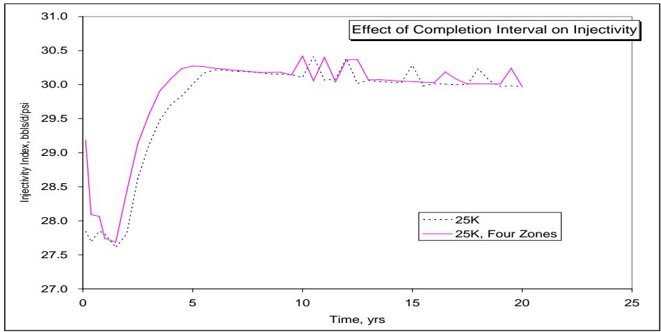
Figure 2 shows that PWRI does result in a significant change in injectivity due to the assumed damage to the external filter cake. Figure 3 shows fracture growth will occur at the rate necessary to rate of water reinjection. A higher injection rate increases injectivity. Figure 2 shows there is little impact on injectivity. Lower permeability results in steeper fracturing. Figure 3 shows there is almost no difference in injectivity between four, 6m perforated intervals across the whole N570 vs. one, 6m interval within the lower portion of the zone.
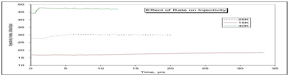 Figure 2: Effect of Rate on Injectivity
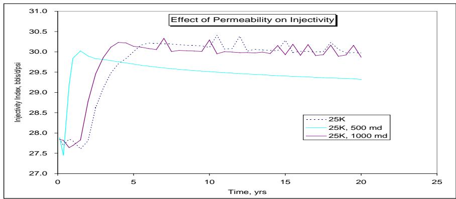 Figure 3: Effect of Permeability on Injectivity
 Figure 4: Effect of Completion Interval on Injectivity
In these section results of modeling analysis based on field data parameters is discussed. Table 1 is regression statistics based on data of scaling index and the other fracturing parameters were obtained from a petroleum regulator in Nigeria and as presented and reported by Idialu 2014. The MATLAB regression model Simulink provides the regression statistics results in
Table 3.0. Table 4.0 is the CHI-SQUARE values of variables of Injectivity with fracturing scale production and formation damage. The regression equation is given by for scaling Index SI to predict scaling tendencies in the field studied as a function of Temperature, pressure, pH and Injection rate.
$$
S I = 1 + A _ {1} T E M P E R A T U R E + A _ {2} P R E S S U R E + A _ {3} P H a f t e r + A _ {4} p H + A _ {5} I N J E C T I O N R A T E
$$
Where $A_{1} = 0.005210855$
$$
A _ {2} = - 9.9 1 E - 0 5 A _ {3} = 0.4 5 6 1 5 0 6 7 8 A _ {4} = - 0.0 2 1 8 4 7 4 2 5 A _ {5} = 3.0 2 E - 0 7 \
$$
Figure 5 shows the effect of each input on the scaling Index (output). The marker on the top right of Figure 6 show that increase the temperature from 80 to 189 make the SID increase by say 0.1 while the next marker show that increase in the pressure make the output to decrease by 0.1. Figure 5 show adjusted SI for Temperature and pH while fig 6 shows adjusted SI for temperature and pressure for any value of pH after. The
SI increases as temperature increase. Figure 7 shows Adjusted SI at any temperature reading and chart indicates the SI decreases as the pressure increases. Figure 8 show interaction of the entire inputs on the output on SI and pH after. It was observed that Injection rate does not really have much effect on the scaling index.
Table 1.0: Regression Statistics
<table><tr><td>Multiple R</td><td>0.9724</td></tr><tr><td>R Square</td><td>0.946</td></tr><tr><td>Adjusted R Square</td><td>0.944</td></tr><tr><td>RMSE</td><td>0.00724</td></tr><tr><td>Error degree of Freedom</td><td>244</td></tr><tr><td>Observations</td><td>250</td></tr></table>
<table><tr><td></td><td>Coefficients</td><td>Standard Error</td><td>t Stat</td><td>P-value</td></tr><tr><td>Intercept</td><td>-1.458805352</td><td>0.186270479</td><td>-7.83165</td><td>1.47E-13</td></tr><tr><td>Temp</td><td>0.005210855</td><td>0.000144843</td><td>35.97596</td><td>1.54E-99</td></tr><tr><td>Pressure</td><td>-9.91E-05</td><td>5.15E-06</td><td>-19.2332</td><td>8.49E-51</td></tr><tr><td>pH</td><td>0.456150678</td><td>0.021363995</td><td>21.35138</td><td>9.30E-58</td></tr><tr><td>pH after</td><td>-0.021847425</td><td>0.004520292</td><td>-4.83319</td><td>2.38E-06</td></tr><tr><td>Injection Rate</td><td>3.02E-07</td><td>9.03E-08</td><td>3.339175</td><td>0.000972</td></tr></table>
Table 2.0: Chi-Square Values for the Variables
<table><tr><td></td><td>P-value</td></tr><tr><td>Intercept</td><td>1.47E-13</td></tr><tr><td>Temp</td><td>1.54E-99</td></tr><tr><td>Pressure</td><td>8.49E-51</td></tr><tr><td>pH</td><td>9.30E-58</td></tr><tr><td>PH after</td><td>2.38E-06</td></tr><tr><td>Injection Rate</td><td>0.000972</td></tr></table>
Table 3.0: T- Stat for the Variables
<table><tr><td></td><td>T Stat</td></tr><tr><td>Intercept</td><td>-7.83165</td></tr><tr><td>Temp</td><td>35.97596</td></tr><tr><td>Pressure</td><td>-19.2332</td></tr><tr><td>pH</td><td>21.35138</td></tr><tr><td>pH after</td><td>-4.83319</td></tr><tr><td>Injection Rate</td><td>3.339175</td></tr></table>
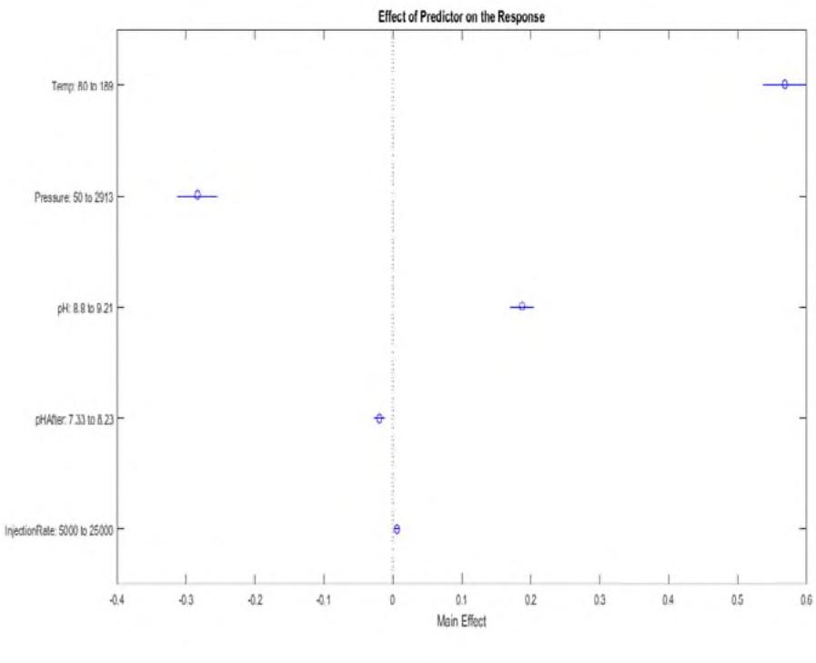
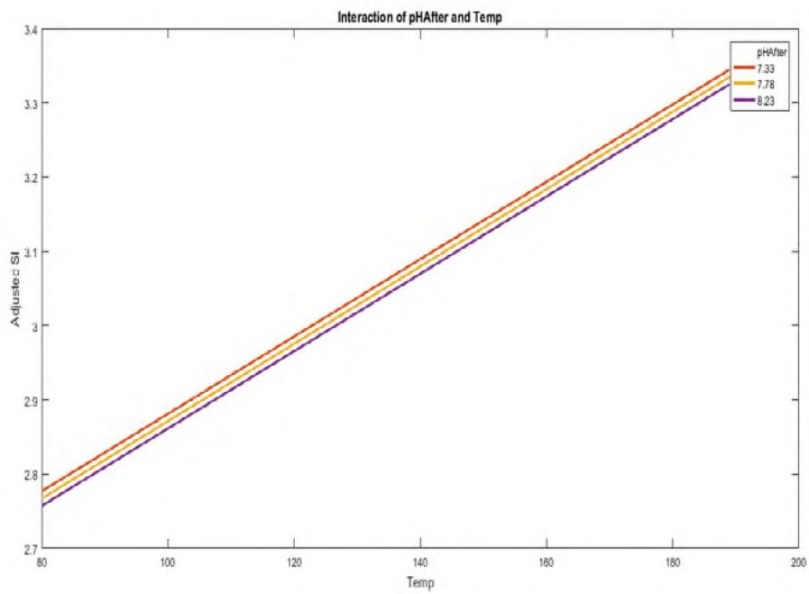 Figure 5: Effect of Predictor on Response
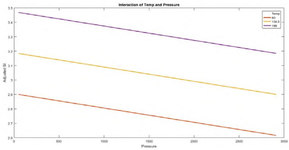 Figure 7: Adjusted SI with Pressure and Temperature
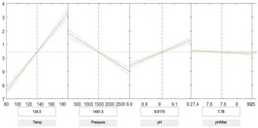 Figure 8: SI with Temperature, Pressure, pH and pH After
Table 6.0 shows the regression statistics based on field data after simulating on MATLAB to generate the regression model or equation with an R square of $97\%$. Table 7.0 is ANOVAs parameters. Table 8.0 shows Chi-Square test based on data on fracturing phenomenon.
Table 6.0: Regression Statistics
<table><tr><td>R Square</td><td>0.997</td></tr><tr><td>Adjusted R Square</td><td>0.9965</td></tr><tr><td>RMSE</td><td>0.00347</td></tr><tr><td>Observations</td><td>60</td></tr></table>
Table 7.0: Anova Paramters
<table><tr><td></td><td>SS</td><td>DF</td><td>MS</td><td>F</td><td>Significance F</td></tr><tr><td>Regression</td><td>0.205440621</td><td>59</td><td>0.003482</td><td></td><td></td></tr><tr><td>Residual</td><td>0.204815196</td><td>7</td><td>0.029259</td><td>2432.721</td><td>4.51E-63</td></tr><tr><td>Total</td><td>0.000625425</td><td>52</td><td>1.20E-05</td><td>0</td><td></td></tr></table>
<table><tr><td></td><td>Coefficients</td><td>Standard Error</td><td>t Stat</td><td>P-value</td></tr><tr><td>Intercept</td><td>0</td><td>0</td><td>NaN</td><td>NaN</td></tr><tr><td>Young's modulus, psi</td><td>1.68E-10</td><td>1.36E-09</td><td>0.124152</td><td>0.901713</td></tr><tr><td>Poisson's Ratio</td><td>2.287796099</td><td>0.025236959</td><td>90.65261</td><td>2.48E-55</td></tr><tr><td>Toughness, psi-in1/2</td><td>0.00141057</td><td>0.000910887</td><td>1.548567</td><td>0.128054</td></tr><tr><td>Pressure, psi</td><td>-7.59E-05</td><td>0.000266942</td><td>-0.28421</td><td>0.777471</td></tr><tr><td>Compressibility, psi-1</td><td>-294.8436887</td><td>279.1197758</td><td>-1.05633</td><td>0.296103</td></tr><tr><td>Permeability, md</td><td>-9.20E-08</td><td>1.46E-06</td><td>-0.06309</td><td>0.949956</td></tr><tr><td>Porosity</td><td>-0.021072465</td><td>0.013422726</td><td>-1.56991</td><td>0.123006</td></tr><tr><td>Formation Fluid Viscosity, cp</td><td>0</td><td>0</td><td>NaN</td><td>NaN</td></tr><tr><td>Coeff of ThermExp (1/R)</td><td>0</td><td>0</td><td>NaN</td><td>NaN</td></tr><tr><td>Temp(F)</td><td>0.00567176</td><td>0.004939851</td><td>1.148164</td><td>0.256591</td></tr><tr><td>Biots Constant</td><td>0</td><td>0</td><td>NaN</td><td>NaN</td></tr></table>
Table 8 are chi square values for variables used to generate P values for intercept, young modulus, psi, Poisson's ratio, toughness, pressure, compressibility, porosity, formation fluid based on data provided in Appendix A Table A3
Table 8.0: Chi-Square Values for Variables
<table><tr><td></td><td>P VALUES</td></tr><tr><td>Intercept</td><td>0</td></tr><tr><td>Young's modulus, psi</td><td>0.901713</td></tr><tr><td>Poisson's Ratio</td><td>2.48E-55</td></tr><tr><td>Toughness, psi-in1/2</td><td>0.128054</td></tr><tr><td>Pressure, psi</td><td>0.777471</td></tr><tr><td>Compressibility, psi-1</td><td>0.296103</td></tr><tr><td>Permeability, md</td><td>0.949956</td></tr><tr><td>Porosity</td><td>0.123006</td></tr><tr><td>Formation Fluid Viscosity, cp</td><td>0</td></tr><tr><td>Coeff of Therm Exp (1/R)</td><td>0</td></tr><tr><td>Temp(F)</td><td>0.256591</td></tr><tr><td>Biots Constant</td><td>0</td></tr></table>
Table 9.0: T Stat for the Variables
<table><tr><td></td><td>T-STAT</td></tr><tr><td>Intercept</td><td>0</td></tr><tr><td>Young's modulus, psi</td><td>0.124152</td></tr><tr><td>Poisson's Ratio</td><td>90.65261</td></tr><tr><td>Toughness, psi-in1/2</td><td>1.548567</td></tr><tr><td>Pressure, psi</td><td>-0.28421</td></tr><tr><td>Compressibility, psi-1</td><td>-1.05633</td></tr><tr><td>Permeability, md</td><td>-0.06309</td></tr><tr><td>Porosity</td><td>-1.56991</td></tr><tr><td>Formation Fluid Viscosity, cp</td><td>0</td></tr><tr><td>Coeff of ThermExp (1/R)</td><td>0</td></tr><tr><td>Temp(F)</td><td>1.148164</td></tr><tr><td>Biots Constant</td><td>0</td></tr></table>
The regression equation to described fracturing phenomenon based on field data is given by $Y = 1 + B1$ YOUNG'S MODULUS + B2POISON\\RATIO + B3TOUGHNESS + B4PRESSURE + B5COMPRESSIBILITY + B6PERMEABILITY + B7POROSITY + B8FORMATION FLUID VISCOSITY + B9COEFF OF THERM EXP + B10TEMP + B11BIOT'S CONSTANT.
Where $Y = \sigma / TVD$
B1=1.68E-10
B2=2.287796099
B3=0.00141057
B4=-7.59E-05
B5=-294.8436887
B6=-9.20E-08
B7=-0.021072465
B8=0
B9=0
B10=0.00567176
B11=0
Table 10: Regression Output Residual = Output-Predicted(Fitted)
<table><tr><td>Observation</td><td>Predicted σHmin/TVD</td><td>Residuals</td></tr><tr><td>1</td><td>1.755176515</td><td>0.002383335</td></tr><tr><td>2</td><td>1.754210421</td><td>0.003282703</td></tr><tr><td>3</td><td>1.754196673</td><td>0.003649684</td></tr><tr><td>4</td><td>1.755563744</td><td>0.002167322</td></tr><tr><td>5</td><td>1.745017372</td><td>0.001815937</td></tr><tr><td>6</td><td>1.707914432</td><td>0.004508949</td></tr><tr><td>7</td><td>1.777649715</td><td>-0.003188842</td></tr><tr><td>8</td><td>1.776929853</td><td>-0.002976813</td></tr><tr><td>9</td><td>1.739535586</td><td>0.001000309</td></tr><tr><td>10</td><td>1.830843069</td><td>-0.007807289</td></tr><tr><td>11</td><td>1.820752739</td><td>-0.005421826</td></tr><tr><td>12</td><td>1.712883501</td><td>0.00694037</td></tr><tr><td>13</td><td>1.760415293</td><td>0.001803846</td></tr><tr><td>14</td><td>1.80893194</td><td>-0.000982362</td></tr><tr><td>15</td><td>1.806798456</td><td>-0.009183584</td></tr><tr><td>16</td><td>1.738907353</td><td>0.004243237</td></tr><tr><td>17</td><td>1.73288535</td><td>0.002451627</td></tr><tr><td>18</td><td>1.77603357</td><td>-0.001781725</td></tr><tr><td>19</td><td>1.77773054</td><td>0.000433982</td></tr><tr><td>20</td><td>1.788037258</td><td>-0.002962604</td></tr><tr><td>21</td><td>1.787112245</td><td>0.00014607</td></tr><tr><td>22</td><td>1.866485352</td><td>-0.001191938</td></tr><tr><td>23</td><td>1.898519512</td><td>-0.000441118</td></tr><tr><td>24</td><td>1.855876948</td><td>-0.001025834</td></tr><tr><td>25</td><td>1.825406668</td><td>-0.003844158</td></tr></table>
Figure 8 shows a match of predicted reservoir production rate and actual production rate and fits into trend analysis for each injectivity run and Fig 9 shows a similar trend for pressure difference is observed. The production rate is marked by peak maxima and minima for each injection run. The tables for both the production index and fracturing phenomenon simulated on MATLAB generated an appropriate model that can be used to analyses the data given. The model generated shows a good fit because the value for the Multiple R (correlation coefficient that tells us how strong the linear relationship is; value of 1 is a perfect positive
relationship while a value of 0 shows no relationship at all), R Squared (statistical measure of how close the data are to the fitted regression line)and the Adjusted R Squared (a modified version of R Squared that has been adjusted for the number of predictors in the model) tends towards 1.0 while the value for the Standard error or the Root Mean Square Error (RMSE) which measures how much error there is between two datasets, compares a predicted value and an observed or known value and the Mean Square Error that measures the average of the squares of the errors or deviation i.e. difference between the estimator and what is estimated. Figure 9 shows the effect of each input on the output (Scaling Index). Increase in temperature will directly lead to an increase in the value of the Scaling Index but reverse is the case for pressure. Figure 9 also shows the interaction between all the inputs on the output. pH after and Injection rate does not really have much effect on the output (Scaling Index).
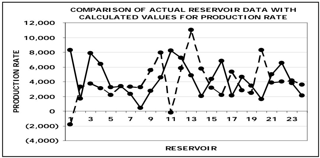 Figure 6: Adjusted SI with Temperature and pH
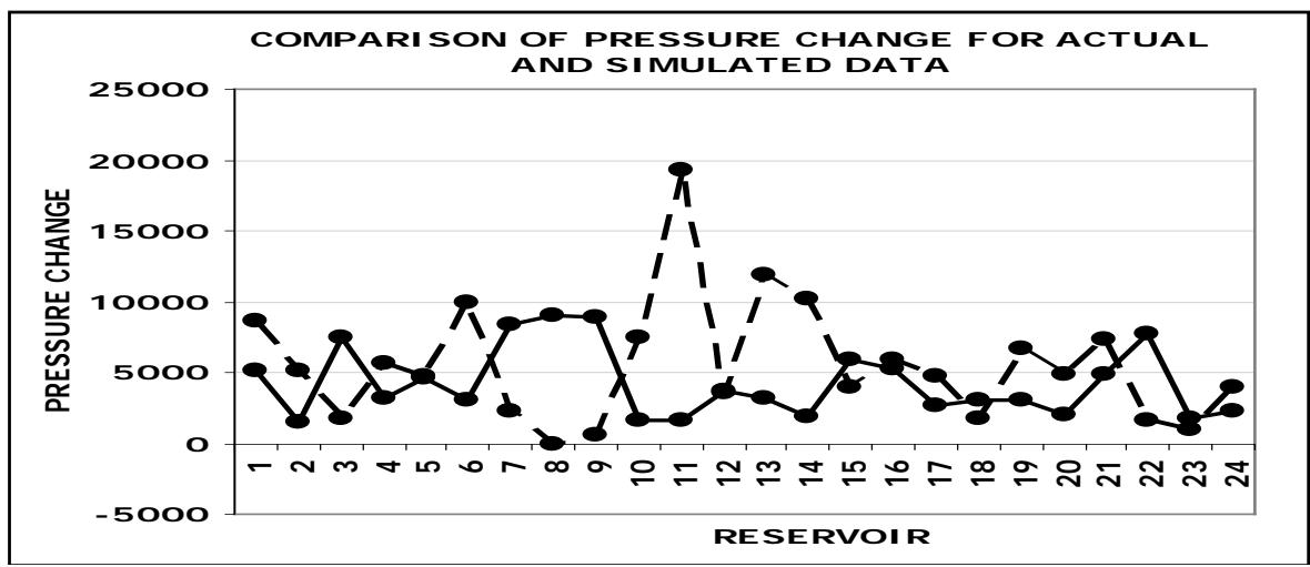 Figure 9: Comparison of Actual Reservoir Data with Simulated Values for Production Rate
Figure 10 and Fig 11 show the frequency distribution statistics for the multiple injection runs with particular classes of production and pressure for multiples simulation injection run. Figure 10 pressure change is shown by peak maxima and minima for injection group 1-24 considered for the reservoir system. A profile of Figure 11 that closely resembles frac pressure data and the peak maxima and minima per injection run
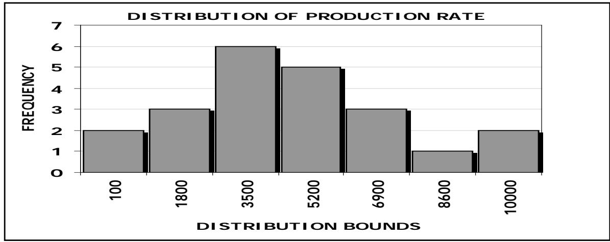 Figure 10: Actual Reservoir Data with Simulated Values for Pressure Change
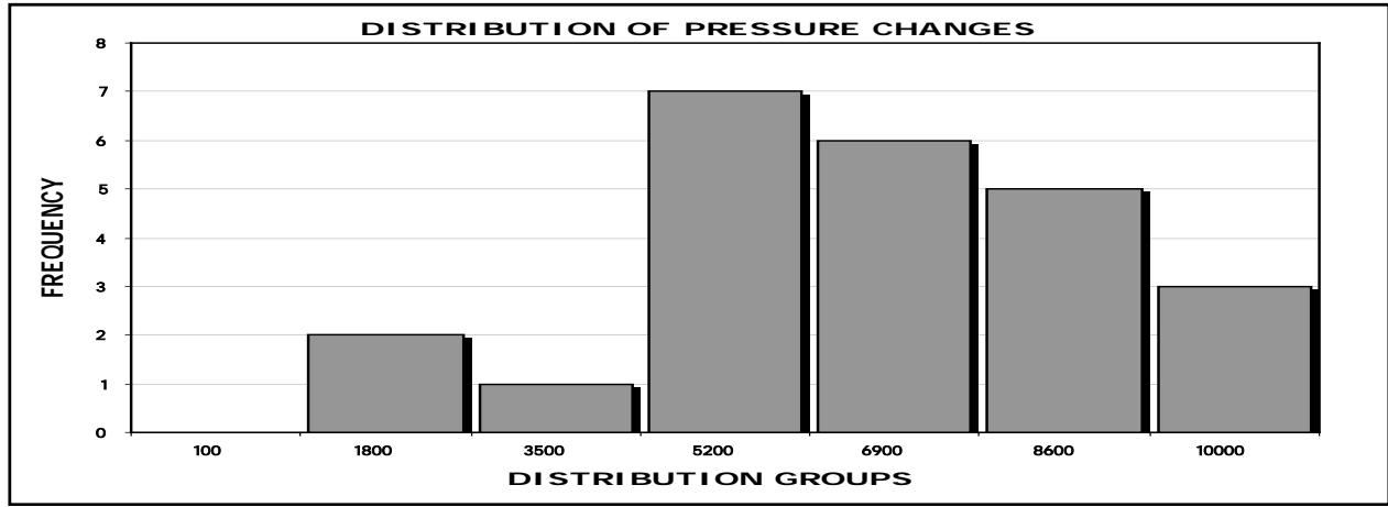 Figure 11: Frequency Distribution of Production Rate for Each Injectivity Group
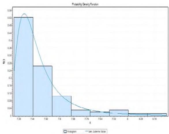
Excel Sheets show the data categorization of variables in Table 5.0. The Monte Carlo model is applied to available reservoir data to study stochastically the pressure performance for several water injection rates for reservoir performance. The pressure changes normalized within a normal distribution thresholds is used to represent different probability scenarios for different injection rate schemes. This calculation also achieved with MS Excel functions required the calculation of the mean and standard deviation of the set of pressure changes for the different reservoirs. The data are represented using simulation random numbers generated to replicate the probability calculated for each of the above pressure change. The results show probabilities is a normal distribution are between 0 and 1, random numbers were generated to lie between 0 and 1 also. MS Excel functions were then written to achieve an inversion of the simulated probability values to pressure changes. To ensure that the simulated values keep dimensions with the actual reservoir data, the mean and standard deviation calculated for the actual data were employed for the inversion. The regression analysis for the field data below is presented in Fig 13.The regression statistics show multiple of R is 0.998476685, R Square is 0.99695569 and Adjusted R square is 0.919622802 and Standard error of 0.003468055 for the 60 observations shows a strong agreement with the Monte Carlo Simulation model and Field data.
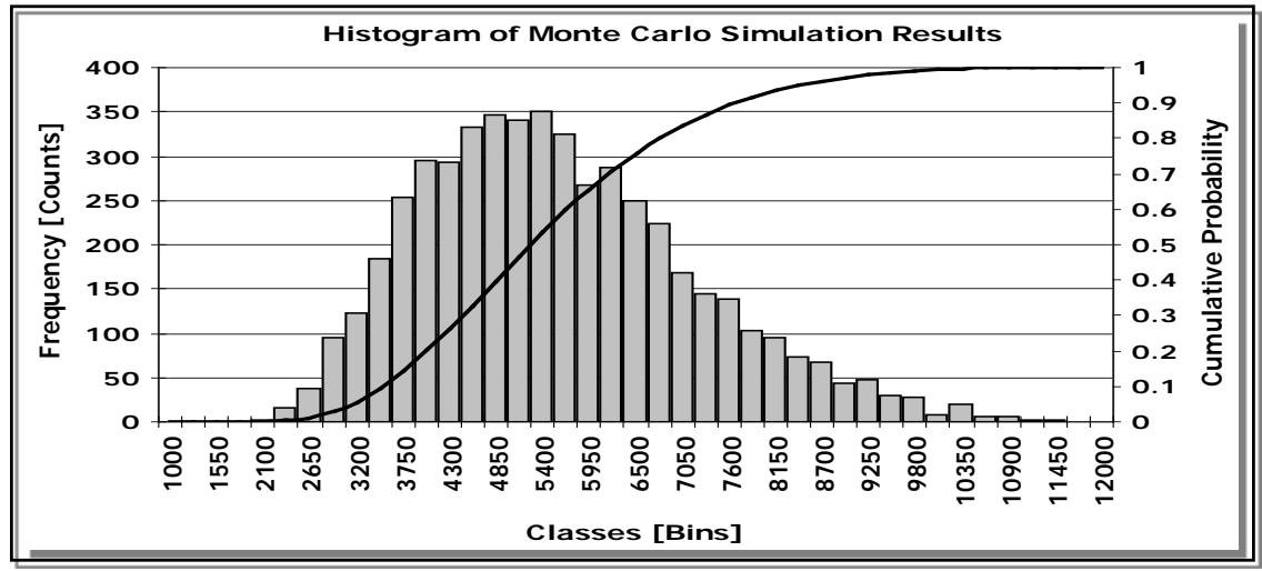 Figure 13: Histogram and Probability Distribution of the Monte Carlo Simulation
This results of simulation of field and production data obtained from the operator such as reservoir data of the study area, produced water parameters quality, factors which are responsible for cake formation and fracture formation is presented in Figure 13. Figure 13 is the data obtained from water reinjection indicates that calcite (calcium carbonate) forms the cake during the water reinjection process. From the graph showing the distribution of water reinjected parameters, it is observed that the amount of calcium and carbonate contained in the produced water is small relative to the other constituents and contributed majorly to cake formation.
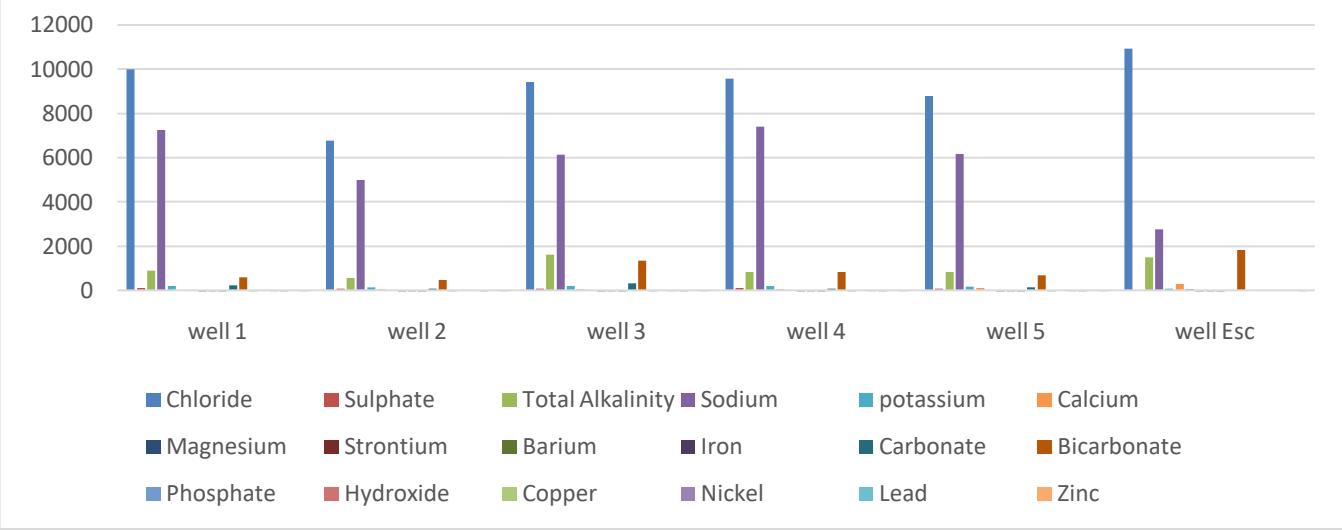 Distribution of Reinjected Water Parameters Figure 13: Chart for Distribution of Produced Water Parameters Quality in the Wells
### b) Regression Analysis Output
Under the null hypothesis, the regression function does not depend on explanatory variables. The individual T statistic is used in calculating the P value which shows the statistical significance of the individual variables. An alpha level of 0.30 was used in this study. A P value less than the alpha level indicate a high statistical significance of the variable. A re-run regression analysis was performed to eliminate variables with high P values and insignificant regression coefficients. In this report, the Scaling Index (SI) which is used as an index of scaling in the formation resulting from produced water reinjection is the dependent variable prediction is based on temperature, pressure, pH, pH after precipitation and Injection rate. A high Multiple R value indicates a strong linear relationship existence. The Adjusted R squared value used in the regression analysis of this study is a multi linear regression. The regression analysis output from the field data is presented in Table 11
Regression Output Scenario 1
Table 11: Regression Analysis Output from Field Data for Well 10 Field X-10ST (Scenario1)
<table><tr><td colspan="2">Regression Statistics</td></tr><tr><td>Multiple R</td><td>0.991167</td></tr><tr><td>R Square</td><td>0.982411</td></tr><tr><td>Adjusted R Square</td><td>0.980412</td></tr><tr><td>Standard Error</td><td>0.003463</td></tr><tr><td>Observations</td><td>50</td></tr></table>
ANOVA
<table><tr><td></td><td>df</td><td>SS</td><td>MS</td><td>F</td><td>Significance F</td></tr><tr><td>Regression</td><td>5</td><td>0.02948</td><td>0.005896</td><td>491.5183</td><td>2.04E-37</td></tr><tr><td>Residual</td><td>44</td><td>0.000528</td><td>1.2E-05</td><td></td><td></td></tr><tr><td>Total</td><td>49</td><td>0.030008</td><td></td><td></td><td></td></tr></table>
<table><tr><td></td><td>Coefficients</td><td>Standard Error</td><td>T Stat</td><td>P-Value</td></tr><tr><td>Intercept</td><td>-2.16204</td><td>0.351959</td><td>-6.14286</td><td>2.08E-07</td></tr><tr><td>Temp</td><td>0.00116</td><td>0.001933</td><td>0.600312</td><td>0.551378</td></tr><tr><td>Pressure</td><td>5.76E-05</td><td>6.76E-05</td><td>0.851287</td><td>0.399219</td></tr><tr><td>pH</td><td>0.55999</td><td>0.037971</td><td>14.74792</td><td>1.22E-18</td></tr><tr><td>pH after</td><td>-0.01215</td><td>0.005895</td><td>-2.06095</td><td>0.045248</td></tr><tr><td>Injection rate</td><td>5.4E-09</td><td>1.6E-07</td><td>0.033702</td><td>0.973267</td></tr></table>
Table 12: Re-Run Regression Output Scenario 1
<table><tr><td colspan="2">Regression Statistics</td></tr><tr><td>Multiple R</td><td>0.991166</td></tr><tr><td>R Square</td><td>0.982411</td></tr><tr><td>Adjusted R Square</td><td>0.980847</td></tr><tr><td>Standard Error</td><td>0.003425</td></tr><tr><td>Observations</td><td>50</td></tr></table>
ANOVA
<table><tr><td></td><td>df</td><td>SS</td><td>MS</td><td>F</td><td>Significance F</td></tr><tr><td>Regression</td><td>4</td><td>0.02948</td><td>0.00737</td><td>628.3449</td><td>7.62E-39</td></tr><tr><td>Residual</td><td>45</td><td>0.000528</td><td>1.17E-05</td><td></td><td></td></tr><tr><td>Total</td><td>49</td><td>0.030008</td><td></td><td></td><td></td></tr></table>
<table><tr><td></td><td>Coefficients</td><td>Standard Error</td><td>t Stat</td><td>P-value</td></tr><tr><td>Intercept</td><td>-2.17122</td><td>0.220229</td><td>-9.85893</td><td>8.1E-13</td></tr><tr><td>Temp</td><td>0.001162</td><td>0.001911</td><td>0.607929</td><td>0.546291</td></tr><tr><td>Pressure</td><td>5.76E-05</td><td>6.68E-05</td><td>0.862559</td><td>0.392954</td></tr><tr><td>pH</td><td>0.561117</td><td>0.017791</td><td>31.54021</td><td>2.5E-32</td></tr><tr><td>pH after</td><td>-0.0123</td><td>0.003793</td><td>-3.24242</td><td>0.002235</td></tr></table>
Table 13: Regression Output Scenario 2
<table><tr><td colspan="2">Regression Statistics</td></tr><tr><td>Multiple R</td><td>0.988244</td></tr><tr><td>R Square</td><td>0.976626</td></tr><tr><td>Adjusted R Square</td><td>0.97397</td></tr><tr><td>Standard Error</td><td>0.003595</td></tr><tr><td>Observations</td><td>50</td></tr></table>
ANOVA
<table><tr><td></td><td>df</td><td>SS</td><td>MS</td><td>F</td><td>Significance F</td></tr><tr><td>Regression</td><td>5</td><td>0.023759</td><td>0.004752</td><td>367.6826</td><td>1.06E-34</td></tr><tr><td>Residual</td><td>44</td><td>0.000569</td><td>1.29E-05</td><td></td><td></td></tr><tr><td>Total</td><td>49</td><td>0.024328</td><td></td><td></td><td></td></tr></table>
<table><tr><td></td><td>Coefficients</td><td>Standard Error</td><td>t Stat</td><td>P-value</td></tr><tr><td>Intercept</td><td>-2.08432</td><td>0.347215</td><td>-6.00297</td><td>3.34E-07</td></tr><tr><td>Temp</td><td>0.002274</td><td>0.002004</td><td>1.13481</td><td>0.262599</td></tr><tr><td>Pressure</td><td>9.93E-06</td><td>6.6E-05</td><td>0.150273</td><td>0.881236</td></tr><tr><td>pH</td><td>0.54543</td><td>0.035752</td><td>15.25596</td><td>3.5E-19</td></tr><tr><td>pH after</td><td>-0.01598</td><td>0.005797</td><td>-2.75678</td><td>0.008465</td></tr><tr><td>Injection rate</td><td>1.79E-08</td><td>1.67E-07</td><td>0.107264</td><td>0.915067</td></tr></table>
Table 14:Rerun Regression Output Scenario 2
<table><tr><td colspan="2">Regression Statistics</td></tr><tr><td>Multiple R</td><td>0.988235186</td></tr><tr><td>R Square</td><td>0.976608784</td></tr><tr><td>Adjusted R Square</td><td>0.97508327</td></tr><tr><td>Standard Error</td><td>0.003517229</td></tr><tr><td>Observations</td><td>50</td></tr></table>
ANOVA
<table><tr><td></td><td>df</td><td>SS</td><td>MS</td><td>F</td><td>Significance F</td></tr><tr><td>Regression</td><td>3</td><td>0.023758938</td><td>0.00791965</td><td>640.183386</td><td>1.67336E-37</td></tr><tr><td>Residual</td><td>46</td><td>0.000569062</td><td>1.2371E-05</td><td></td></tr><tr><td>Total</td><td>49</td><td>0.024328</td><td></td><td></td></tr><tr><td></td><td>Coefficients</td><td>Standard Error</td><td>t Stat</td><td>P-value</td></tr><tr><td>Intercept</td><td>-2.134068821</td><td>0.15778</td><td>-13.525597</td><td>1.2145E-17</td></tr><tr><td>Temp</td><td>0.002584819</td><td>6.86134E-05</td><td>37.6722122</td><td>3.1818E-36</td></tr><tr><td>pH</td><td>0.548701518</td><td>0.016598371</td><td>33.057553</td><td>1.0517E-33</td></tr><tr><td>pH after</td><td>-0.016524371</td><td>0.003773413</td><td>-4.3791581</td><td>6.8162E-05</td></tr></table>
d) Regression Analysis Output from Field Data for Well 13 Field X-13HST (Scenario 3) Table 15 is the regression output for scenario 3
Table 15: Regression Output Scenario 3
<table><tr><td colspan="2">Regression Statistics</td></tr><tr><td>Multiple R</td><td>0.975719</td></tr><tr><td>R Square</td><td>0.952028</td></tr><tr><td>Adjusted R Square</td><td>0.946577</td></tr><tr><td>Standard Error</td><td>0.005013</td></tr><tr><td>Observations</td><td>50</td></tr></table>
ANOVA
<table><tr><td></td><td>df</td><td>SS</td><td>MS</td><td>F</td><td>Significance F</td></tr><tr><td>Regression</td><td>5</td><td>0.021944</td><td>0.004389</td><td>174.6405</td><td>7.53E-28</td></tr><tr><td>Residual</td><td>44</td><td>0.001106</td><td>2.51E-05</td><td></td><td></td></tr><tr><td>Total</td><td>49</td><td>0.02305</td><td></td><td></td><td></td></tr></table>
<table><tr><td></td><td>Coefficients</td><td>Standard Error</td><td>t Stat</td><td>P-value</td><td>Lower 95%</td></tr><tr><td>Intercept</td><td>-3.44031</td><td>0.667229</td><td>-5.15611</td><td>5.75E-06</td><td>-4.78502</td></tr><tr><td>Temp</td><td>0.006318</td><td>0.003042</td><td>2.077188</td><td>0.043654</td><td>0.000188</td></tr><tr><td>Pressure</td><td>-0.00011</td><td>9.94E-05</td><td>-1.09295</td><td>0.280366</td><td>-0.00031</td></tr><tr><td>pH</td><td>0.693906</td><td>0.070894</td><td>9.788002</td><td>1.29E-12</td><td>0.551029</td></tr><tr><td>pH after</td><td>-0.06126</td><td>0.012195</td><td>-5.0229</td><td>8.94E-06</td><td>-0.08583</td></tr><tr><td>Injection rate</td><td>5.18E-07</td><td>2.13E-07</td><td>2.430296</td><td>0.019233</td><td>8.85E-08</td></tr></table>
Table 16:Rerun Regression Output Scenario 3
<table><tr><td colspan="2">Regression Statistics</td></tr><tr><td>Multiple R</td><td>0.972414</td></tr><tr><td>R Square</td><td>0.945589</td></tr><tr><td>Adjusted R Square</td><td>0.940752</td></tr><tr><td>Standard Error</td><td>0.005279</td></tr><tr><td>Observations</td><td>50</td></tr></table>
ANOVA
<table><tr><td></td><td>df</td><td>SS</td><td>MS</td><td>F</td><td>Significance F</td></tr><tr><td>Regression</td><td>4</td><td>0.021796</td><td>0.005449</td><td>195.5079</td><td>7.96E-28</td></tr><tr><td>Residual</td><td>45</td><td>0.001254</td><td>2.79E-05</td><td></td><td></td></tr><tr><td>Total</td><td>49</td><td>0.02305</td><td></td><td></td><td></td></tr></table>
<table><tr><td></td><td>Coefficients</td><td>Standard Error</td><td>t Stat</td><td>P-value</td><td>Lower 95%</td></tr><tr><td>Intercept</td><td>-4.60358</td><td>0.489533</td><td>-9.40402</td><td>3.44E-12</td><td>-5.58955</td></tr><tr><td>Temp</td><td>0.008126</td><td>0.003106</td><td>2.616268</td><td>0.012059</td><td>0.00187</td></tr><tr><td>Pressure</td><td>-0.00015</td><td>0.000103</td><td>-1.50154</td><td>0.1402</td><td>-0.00036</td></tr><tr><td>pH</td><td>0.827179</td><td>0.047315</td><td>17.48224</td><td>1.1E-21</td><td>0.731881</td></tr><tr><td>pH after</td><td>-0.08656</td><td>0.006688</td><td>-12.9415</td><td>9.01E-17</td><td>-0.10003</td></tr></table>
SI = -4.60358 + 0.008126 * Temperature - 0.00015 * Pressure + 0.827179 * pH - 0.08656 * pH after precipitation
### e) Regression Analysis Output from Field Data for Well 18 Field X-18ST (Scenario 4)
Table 17: Regression Output Scenario 4
<table><tr><td colspan="2">Regression Statistics</td></tr><tr><td>Multiple R</td><td>0.997422</td></tr><tr><td>R Square</td><td>0.99485</td></tr><tr><td>Adjusted R Square</td><td>0.994265</td></tr><tr><td>Standard Error</td><td>0.003114</td></tr><tr><td>Observations</td><td>50</td></tr></table>
ANOVA
<table><tr><td></td><td>df</td><td>SS</td><td>MS</td><td>F</td><td>Significance F</td></tr><tr><td>Regression</td><td>5</td><td>0.082423</td><td>0.016485</td><td>1699.89</td><td>3.83E-49</td></tr><tr><td>Residual</td><td>44</td><td>0.000427</td><td>9.7E-06</td><td></td><td></td></tr><tr><td>Total</td><td>49</td><td>0.08285</td><td></td><td></td><td></td></tr></table>
<table><tr><td></td><td>Coefficients</td><td>Standard Error</td><td>t Stat</td><td>P-value</td></tr><tr><td>Intercept</td><td>-1.15459</td><td>0.32674</td><td>-3.53367</td><td>0.000977</td></tr><tr><td>Temp</td><td>-0.00441</td><td>0.001934</td><td>-2.28196</td><td>0.027384</td></tr><tr><td>Pressure</td><td>0.000274</td><td>7.36E-05</td><td>3.71952</td><td>0.000562</td></tr><tr><td>pH</td><td>0.491024</td><td>0.034478</td><td>14.24165</td><td>4.38E-18</td></tr><tr><td>pH after</td><td>-0.00445</td><td>0.006946</td><td>-0.64022</td><td>0.525348</td></tr><tr><td>Injection rate</td><td>2.42E-08</td><td>1.18E-07</td><td>0.204374</td><td>0.839004</td></tr></table>
SI = -1.15459 - 0.00441 * Temperature + 0.000274 * Pressure + 0.491024 * pH - 0.00445 * pH after precipitation + 2.42E-08 * Injection Rate
Table 18:Rerun Regression Output Scenario 4
<table><tr><td colspan="2">Regression Statistics</td></tr><tr><td>Multiple R</td><td>0.997314</td></tr><tr><td>R Square</td><td>0.994636</td></tr><tr><td>Adjusted R Square</td><td>0.994286</td></tr><tr><td>Standard Error</td><td>0.003108</td></tr><tr><td>Observations</td><td>50</td></tr></table>
ANOVA
<table><tr><td></td><td>df</td><td>SS</td><td>MS</td><td>F</td><td>Significance F</td></tr><tr><td>Regression</td><td>3</td><td>0.082406</td><td>0.027469</td><td>2843.115</td><td>3.29E-52</td></tr><tr><td>Residual</td><td>46</td><td>0.000444</td><td>9.66E-06</td><td></td><td></td></tr><tr><td>Total</td><td>49</td><td>0.08285</td><td></td><td></td><td></td></tr></table>
<table><tr><td></td><td>Coefficients</td><td>Standard Error</td><td>t Stat</td><td>P-value</td></tr><tr><td>Intercept</td><td>-1.10102</td><td>0.20865</td><td>-5.27688</td><td>3.45E-06</td></tr><tr><td>Temperature</td><td>-0.00485</td><td>0.001865</td><td>-2.59896</td><td>0.012524</td></tr><tr><td>Pressure</td><td>0.00029</td><td>7.15E-05</td><td>4.056664</td><td>0.000191</td></tr><tr><td>pH</td><td>0.485192</td><td>0.01795</td><td>27.0295</td><td>7.08E-30</td></tr></table>
### f) Regression Analysis Output from Field Data for Well 26 Field X-26 (Scenario 5)
Table 19: Regression Output Scenario 5
<table><tr><td colspan="2">Regression Statistics</td></tr><tr><td>Multiple R</td><td>0.986538</td></tr><tr><td>R Square</td><td>0.973258</td></tr><tr><td>Adjusted R Square</td><td>0.970219</td></tr><tr><td>Standard Error</td><td>0.00287</td></tr><tr><td>Observations</td><td>50</td></tr></table>
ANOVA
<table><tr><td></td><td>df</td><td>SS</td><td>MS</td><td>F</td><td>Significance F</td></tr><tr><td>Regression</td><td>5</td><td>0.01319</td><td>0.002638</td><td>320.2661</td><td>2.03E-33</td></tr><tr><td>Residual</td><td>44</td><td>0.000362</td><td>8.24E-06</td><td></td><td></td></tr><tr><td>Total</td><td>49</td><td>0.013552</td><td></td><td></td><td></td></tr></table>
<table><tr><td></td><td>Coefficients</td><td>Standard Error</td><td>t Stat</td><td>P-value</td></tr><tr><td>Intercept</td><td>-0.00585</td><td>0.425917</td><td>-0.01373</td><td>0.989111</td></tr><tr><td>Temp</td><td>-0.00014</td><td>0.001721</td><td>-0.08203</td><td>0.934997</td></tr><tr><td>Pressure</td><td>6.6E-05</td><td>5.65E-05</td><td>1.167831</td><td>0.249164</td></tr><tr><td>pH</td><td>0.32345</td><td>0.047651</td><td>6.787871</td><td>2.34E-08</td></tr><tr><td>pH after</td><td>0.003212</td><td>0.009405</td><td>0.341508</td><td>0.734347</td></tr><tr><td>Injection rate</td><td>7.46E-08</td><td>9.11E-08</td><td>0.818697</td><td>0.417372</td></tr></table>
Table 20:Rerun Regression Output Scenario 5
<table><tr><td colspan="2">Regression Statistics</td></tr><tr><td>Multiple R</td><td>0.986282</td></tr><tr><td>R Square</td><td>0.972753</td></tr><tr><td>Adjusted R Square</td><td>0.971594</td></tr><tr><td>Standard Error</td><td>0.002803</td></tr><tr><td>Observations</td><td>50</td></tr></table>
ANOVA
<table><tr><td></td><td>df</td><td>SS</td><td>MS</td><td>F</td><td>Significance F</td></tr><tr><td>Regression</td><td>2</td><td>0.013183</td><td>0.006591</td><td>838.9829</td><td>1.7E-37</td></tr><tr><td>Residual</td><td>47</td><td>0.000369</td><td>7.86E-06</td><td></td><td></td></tr><tr><td>Total</td><td>49</td><td>0.013552</td><td></td><td></td><td></td></tr></table>
<table><tr><td></td><td>Coefficients</td><td>Standard Error</td><td>t Stat</td><td>P-value</td><td>Lower 95%</td></tr><tr><td>Intercept</td><td>-0.18532</td><td>0.252548</td><td>-0.73382</td><td>0.466704</td><td>-0.69339</td></tr><tr><td>Pressure</td><td>6.37E-05</td><td>3.56E-06</td><td>17.89608</td><td>1.29E-22</td><td>5.65E-05</td></tr><tr><td>pH</td><td>0.344549</td><td>0.027479</td><td>12.5384</td><td>1.33E-16</td><td>0.289267</td></tr></table>
$$
S I = - 0. 1 8 5 3 2 + 6. 3 7 E - 0 5 * P r e s s u r e + 0. 3 4 4 5 4 9 * p H
$$
### g) Regression Analysis Output from Field Data for Field X (Scenario 6)
#### FIELD X
This scenario considers altogether the previous scenarios.
Table 21: Regression Output Scenario 6
<table><tr><td colspan="2">Regression Statistics</td></tr><tr><td>Multiple R</td><td>0.972378</td></tr><tr><td>R Square</td><td>0.945518</td></tr><tr><td>Adjusted R Square</td><td>0.944402</td></tr><tr><td>Standard Error</td><td>0.007245</td></tr><tr><td>Observations</td><td>250</td></tr></table>
ANOVA
<table><tr><td></td><td>df</td><td>SS</td><td>MS</td><td>F</td><td>Significance F</td></tr><tr><td>Regression</td><td>5</td><td>0.222256</td><td>0.044451</td><td>846.9089</td><td>6.3E-152</td></tr><tr><td>Residual</td><td>244</td><td>0.012807</td><td>5.25E-05</td><td></td><td></td></tr><tr><td>Total</td><td>249</td><td>0.235062</td><td></td><td></td><td></td></tr><tr><td></td><td>Coefficients</td><td>Standard Error</td><td>t Stat</td><td>P-value</td></tr><tr><td>Intercept</td><td>-1.45881</td><td>0.18627</td><td>-7.83165</td><td>1.47E-13</td></tr><tr><td>Temp</td><td>0.005211</td><td>0.000145</td><td>35.97596</td><td>1.5E-99</td></tr><tr><td>Pressure</td><td>-9.9E-05</td><td>5.15E-06</td><td>-19.2332</td><td>8.49E-51</td></tr><tr><td>pH</td><td>0.456151</td><td>0.021364</td><td>21.35138</td><td>9.3E-58</td></tr><tr><td>pH after</td><td>-0.02185</td><td>0.00452</td><td>-4.83319</td><td>2.38E-06</td></tr><tr><td>Injection rate</td><td>3.02E-07</td><td>9.03E-08</td><td>3.339175</td><td>0.000972</td></tr></table>
Table 22: Regression Analysis on Rock Properties
<table><tr><td colspan="2">Regression Statistics</td></tr><tr><td>Multiple R</td><td>0.999199</td></tr><tr><td>R Square</td><td>0.998399</td></tr><tr><td>Adjusted R Square</td><td>0.998218</td></tr><tr><td>Standard Error</td><td>8.593554</td></tr><tr><td>Observations</td><td>60</td></tr></table>
ANOVA
<table><tr><td></td><td>df</td><td>SS</td><td>MS</td><td>F</td></tr><tr><td>Regression</td><td>6</td><td>2440890</td><td>406814.94</td><td>5508.727</td></tr><tr><td>Residual</td><td>53</td><td>3914.006</td><td>73.849176</td><td></td></tr><tr><td>Total</td><td>59</td><td>2444804</td><td></td><td></td></tr></table>
<table><tr><td></td><td>Coefficients</td><td>Standard Error</td><td>t Stat</td><td>P-value</td></tr><tr><td>Intercept</td><td>-4151.74</td><td>79.70977</td><td>-52.08573</td><td>3.36E-47</td></tr><tr><td>Young's modulus, psi</td><td>-5.4E-07</td><td>3.29E-06</td><td>-0.163835</td><td>0.870484</td></tr><tr><td>Poisson's Ratio</td><td>5077.193</td><td>62.49606</td><td>81.240204</td><td>2.65E-57</td></tr><tr><td>Pressure, psi</td><td>1.892506</td><td>0.024376</td><td>77.637016</td><td>2.87E-56</td></tr><tr><td>Compressibility, psi-1</td><td>-576349</td><td>690414.7</td><td>-0.834786</td><td>0.407585</td></tr><tr><td>Permeability, md</td><td>0.006449</td><td>0.002004</td><td>3.2186398</td><td>0.0022</td></tr><tr><td>Porosity</td><td>-38.5441</td><td>33.04645</td><td>-1.166361</td><td>0.24869</td></tr></table>
Table 23: Re-Run Regression Analysis on Rock Properties
<table><tr><td colspan="2">Regression Statistics</td></tr><tr><td>Multiple R</td><td>0.999199</td></tr><tr><td>R Square</td><td>0.998398</td></tr><tr><td>Adjusted R Square</td><td>0.99825</td></tr><tr><td>Standard Error</td><td>8.515768</td></tr><tr><td>Observations</td><td>60</td></tr></table>
ANOVA
<table><tr><td></td><td>df</td><td>SS</td><td>MS</td><td>F</td><td>Significance F</td></tr><tr><td>Regression</td><td>5</td><td>2440887.7</td><td>488177.5</td><td>6731.783</td><td>3.77E-74</td></tr><tr><td>Residual</td><td>54</td><td>3915.9886</td><td>72.51831</td><td></td><td></td></tr><tr><td>Total</td><td>59</td><td>2444803.7</td><td></td><td></td><td></td></tr></table>
<table><tr><td></td><td>Coefficients</td><td>Standard Error</td><td>t Stat</td><td>P-value</td></tr><tr><td>Intercept</td><td>-4157.12</td><td>71.976823</td><td>-57.7564</td><td>3.14E-50</td></tr><tr><td>Poisson's Ratio</td><td>5074.787</td><td>60.197479</td><td>84.30232</td><td>5.32E-59</td></tr><tr><td>Pressure, psi</td><td>1.893951</td><td>0.0225194</td><td>84.10327</td><td>6.04E-59</td></tr><tr><td>Compressibility, psi-1</td><td>-541275</td><td>650444.08</td><td>-0.83216</td><td>0.408983</td></tr><tr><td>Permeability, md</td><td>0.006473</td><td>0.0019803</td><td>3.268503</td><td>0.001884</td></tr><tr><td>Porosity</td><td>-34.6017</td><td>22.444932</td><td>-1.54162</td><td>0.129005</td></tr></table>
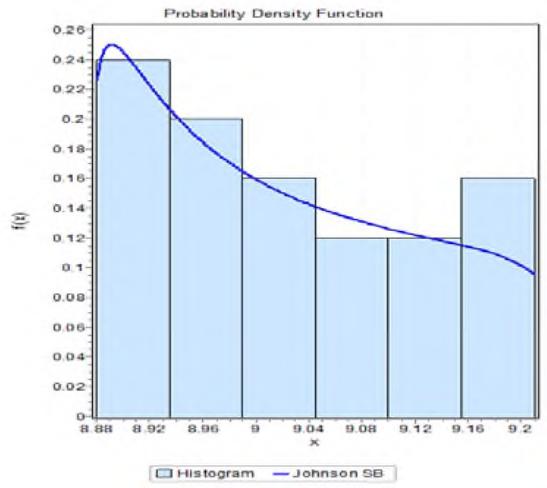
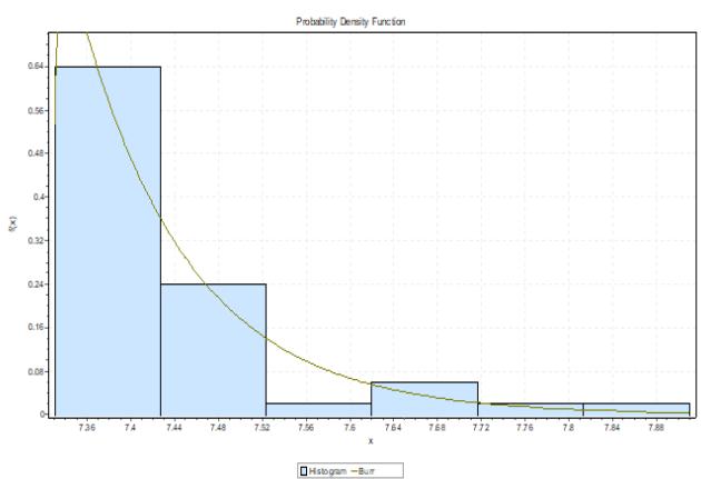
### i) Monte Carlo Simulation
The Monte Carlo Simulation which are the probability distribution defines the best fit of the independent variables where each scenario was described.
## i. Monte Carlo Probability Distributions
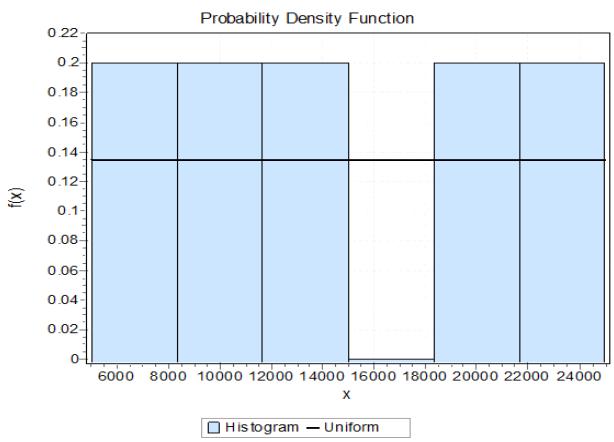
 Scenario 1 - WELL 10 Temperature (Uniform) □ Histogram—Uniform
 Pressure (Uniform) □ Histogram—Uniform
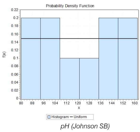 Figure 12: Frequency Distributions of Pressure Changes for Each Injectivity Group
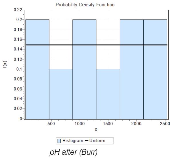
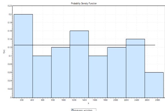
 Injection Rate (uniform) Figure 19: Probability Distribution Functions for Variables in Predicting SI in Well 18
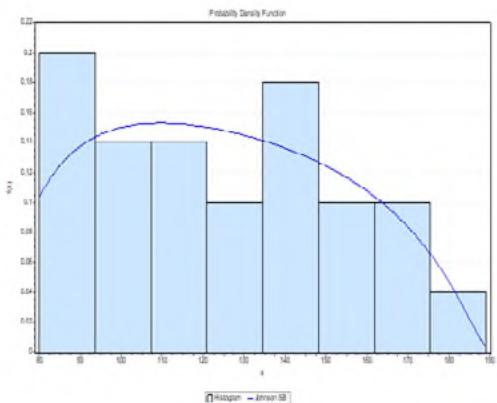 Temperature (Johnson SB) pH (Johnson SB)
 Pressure (Uniform) pH after (Gen. Extreme Value)
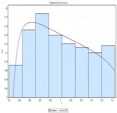
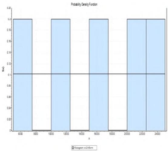 Injection Rate (Uniform) Figure 20: Probability distribution functions for variables in predicting SI in Field X
# j) Simulations of Effects of Cake
The injector well performance was evaluated based on the injectivity index. An average value of 15,000 bbl/d was used as injection rate in calculating injectivity index based on average injection rates in the various wells of the Nigerian oil field. Based on the estimated values of Scaling Index (SI) from the Monte
Carlo Simulation, Injectivity Index was then determined and various plots created.
In a number of thirty (30) simulation plots to model the effects of cake formation on injector well performance, it was observed in Scenario 1, that twenty-five (25) simulation plots indicated a decreasing trend in well performance, four (4) indicated a constant trend in the injection well performance and one (1) indicated an increasing trend in well performance based on increasing cake formation. In Scenario 2, it was observed that twenty-eight (28) simulation plots indicated a decreasing trend in well performance, zero (0) indicated a constant trend in the injection well performance and two (2) indicated an increasing trend in well performance based on increasing cake formation. In Scenario 3, it was observed that twenty-seven (27) simulation plots indicated a decreasing trend in well performance, and three (3) indicated a constant trend in the injection well performance based on increasing cake formation. In Scenario 4, it was observed that twenty-six (26) simulation plots indicated a decreasing trend in well performance, two (2) indicated a constant trend in the injection well performance and two (2) indicated an increasing trend in well performance based on increasing cake formation. In Scenario 5, it was observed that twenty-five (25) simulation plots indicated a decreasing trend in well
performance, and five (5) indicated an increasing trend in well performance based on increasing cake formation. In Scenario 6, it was observed that all thirty (30) simulation plots indicated a decreasing trend in well performance, based on increasing cake formation. A tabulated expression is seen in Appendix B1. Appendix B1 show the simulations that there were occasions when Injectivity index was very high which indicated high well performance before a decline. This could be likened to a result of computer generated low values of flowing wellbore pressure.
### k) Simulations of Effect of Fracturing on Injector Well Performance
The table below shows the simulation data for evaluating the effect of fracturing on the Injector Well Performance for a Field Y in the Gulf of Mexico.
Table 24: Simulation Data for Fracturing Effect on Injector Well Performance in Field Y Gulf of Mexico
#### Parameter
Reservoir Pressure, Pe
Maximum Shear Stress
Fluid Shear Stress
Wellbore Flowing Pressure, $P_{wf}$
Injection Rate
#### Values
5000 psia
2500 psi
#### 1671.315 psi
Simulated
15,000 bbl/d
A $K_{\mathrm{fs}}$ value of 0 indicates rock fracture propagation while a $K_{\mathrm{fs}}$ value of 1 indicates least fracture propagation. A simulation plot of Injectivity Index against rock fracture production Rate is illustrated below.
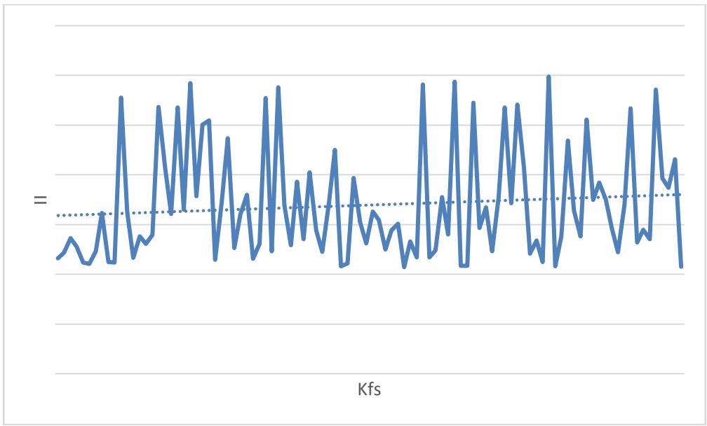 Figure 21: Simulation Plot (10) for Field Y in Gulf of Mexico
To model the effect of rock fracture propagation rate on Injector Well Performance, fifty (50) simulation plots were run. It was observed that seven plots (7) indicated a decline, seven (7) indicated a constant and thirty-six (36) indicated an increase in Injector Well
Performance with increasing value of Kfs i.e. decreasing rock fracture propagation rate which implies more fluid flow.
## V. CONCLUSION
In the formation of the hypothesis, five explanatory variables: Temperature, Pressure, pH, pH after precipitation and Injection rate were used to create a statistical regression analysis model for the prediction of Scaling Index (SI). Hence, it is suggested that all the five explanatory variables be used in creating a model. The Monte Carlo simulations ran all indicated SI values greater than 0 in all scenarios indicating potential for scale formation. SI = < 0 indicates no potential for scaling and SI = > 0 indicates scaling potential. In predicting fracturing, the rock shear stress and maximum shear stress were evaluated and fracturing can occur when the fluid shear stress is greater than the
### ACKNOWLEDGEMENTS
Generating HTML Viewer...
References
35 Cites in Article
Z Khatib (2007). Produced Water Management: Is it a Future Legacy or a Business Opportunity for Field Development.
A Abou-Sayed,K Zaki,G Wang,M Sarfare (2005). A Mechanistic Model for Formation Damage and Fracture Propagation during Water Injection.
Shutong Pang,M Sharma (1994). A Model for Predicting Injectivity Decline in Water-Injection Wells.
S Pang,M Sharma (1997). A Model for Predicting Injectivity Decline in Water Injection Wells.
R Farajzadeh (2002). Produced Water Re-injection (PWRI) -An Experimental Investigation into Internal Filtration and External Cake Buildup.
I Obe,T Fashanu,P Idialu,T Akintola,K Abhulimen (2017). Produced Water Re-injection in a Non-Fresh Water Aquifer with Geochemical Reaction, Hydrodynamic Molecular Dispersion and Adsorption Kinetics Controlling: Model Development and Numerical Simulation.
Kingsley Abhulimen,S Fashanu,Peter Idialu (2018). Modeling fracturing pressure parameters in predicting injector performance and permeability damage in subsea well completion multi-reservoir system.
R Agut,M G. Edwards,S Verma,K Aziz (1998). Flexible Streamline-Potential Grids with Discretization on Highly Distorted Cells.
Z You,A Kalantariasl,K Schulze,J Storz,C Burmester,S Künckeler,P Bedrikovetsky (2016). Injectivity Impairment During Produced Water Disposal into Low-Permeability Völkersen Aquifer (Compressibility and Reservoir Boundary Effects).
Ahmad Ghassemi,Sergejtarasvos (2015). Analysis of Fracture propagation under Thermal Stress in Geothermal Reservoirs.
K Aziz (1983). Algebraic Multigrid (AMG): Experiences and Comparisons.
K Aziz,A Settari (1979). Petroleum Reservoir Simulation.
Ivar Aavatsmark,Tor Barkve,Trond Mannseth (1997). Control-Volume Discretization Methods for 3D Quadrilateral Grids in Inhomogeneous, Anisotropic Reservoirs.
J Barkman,D Davidson (1972). Measuring Water Quality and Predicting Well Impairment.
Zdeněk Bažant,Hideomi Ohtsubo,Kazuo Aoh (1979). Stability and post-critical growth of a system of cooling or shrinkage cracks.
Pavel Bedrikovetsky,Pavel Bedrikovetsky,Claudio Furtado,Alexandre Siqueira,Antonio De Souza (2007). A Comprehensive Model for Injectivity Decline Prediction During PWRI.
S Buckley,M Leverett (1942). Mechanism of Fluid Displacement in Sands.
F Erdogan (1974). Principles of Fracture Mechanics.
Hooman Fallah,Sara Sheydai (2013). Drilling Operation and Formation Damage.
A Ghassemi,S Tarasovs,Null- Cheng (2007). A 3-D study of the effects of thermomechanical loads on fracture slip in enhanced geothermal reservoirs.
B Hustedt,D Zwarts,H Bjoerndal,R Mastry,P Van Den Hoek (2006). Induced Fracturing in Reservoir Simulation: Application of a New Coupled Simulator to Water Flooding Field Examples.
Tomihisa Iwasaki (1937). Some Notes on Sand Filtration.
P Idialu (2014). Modeling of adsorption kinetics, hydrodynamic dispersion and geochemical reaction of produced water reinjection (PWRI) in hydrocarbon aquifer.
X Li,L Cui,J-C Roegiers (1998). Thermoporoelastic modelling of wellbore stability in non-hydrostatic stress field.
Maira Oliveira,Alexandre Vaz,Fernando Siqueira,Yulong Yang,Zhenjiang You,Pavel Bedrikovetsky (2014). Slow migration of mobilised fines during flow in reservoir rocks: Laboratory study.
Qihong Feng,Hongwei Chen,Xiang Wang,Sen Wang,Zenglin Wang,Yong Yang,Shaoxian Bing (2016). Well control optimization considering formation damage caused by suspended particles in injected water.
Z You,A Kalantariasl,K Schulze,J Storz,C Burmester,S Künckeler,P Bedrikovetsky (2016). Injectivity Impairment During Produced Water Disposal into Low-Permeability Völkersen Aquifer (Compressibility and Reservoir Boundary Effects).
A Castellini,M G. Edwards,L J. Durlofsky (2000). Flow based modules for grid generation in two and three dimensions.
X Wang,S Chen,Y Han,Y Abousleiman (2024). A Graph-Based Drained Wellbore Stability Analysis in Mohr-Coulomb Rock Formation Under Hydrostatic in Situ Stress Field.
B Meyer (2003). Leveling Sweet Lake Geopressured Well Site.
A Satter,J Varnon,M Hoang (1994). Integrated Reservoir Management.
D Schiozer,Khalid Aziz (1994). Use of Domain Decomposition for Simultaneous Simulation of Reservoir and Surface Facilities.
S Verma,K Aziz (1996). Two- and Three-Dimensional Flexible Grids for Reservoir Simulation.
Santosh Verma,Khalid Aziz (1997). A Control Volume Scheme for Flexible Grids in Reservoir Simulation.
M Wyllie (1962). ex-nomination 24, 27, 31–2; in humanism: Catholic 69; technological French translation 6, 33 70; traditional 73 hyperconformity 2–3 design 81–3, 118–19; Bauhaus 71 dropping out 101–3 Internet 99; cybercops 101; cyberculture and business 9 effraction 90; break and entry 86; see implosion 4, 50, 94–8, 111, 122; and also symbolic exchange consciousness 83; and nationalism Einsteinism 18, 23 103 electricity: light 48–9; and language 49; and implosion 96–7 Japan 1 Eskimos 107–8, 110–11, 116 Jesus 104, 116 Expo ’67 5, 59, 92, 100; Christian j’explique rien 5 Pavilion 104; Québec Pavilion 5, 92 Expo ’92 4 Latin character 44; Gallic 7, 56, 57, 58; extensions of man 68, 85, 90; mediatic Gallicized name 53; opposed to 58 53; outering 12 liberalism 46, 103–4; cool media 105 families 101; human 102; mafia 101; M et M 58 McLuhan’s 56; commune-ist 116 Ma – Ma – Ma – Ma 58–9 figure and ground 21, 26, 35 Mac 53, 54, 58; Macbeth 54; MacBett French McLuhan 1, 2, 20, 76–8, 98; 57; Macheath 54; Big Mac 58 new 77 Le mac 62 Mack 55 galaxies 39, 41–2, 44, 99, 109, 116; McLuhan: Counterblast 118; Du and detribalization 107; Gutenberg cliché à l’archétype 119–20; 4, 14, 18, 26, 42–3, 47, 51, 85, Explorations in Communication 121; galactic shifts 38; galaxie 16; From Cliché to Archetype 119; MacLuhan 56; and tribalism 106 La galaxie Gutenberg 4, 44; The gap in historical experience 8, 91–2, Gutenberg Galaxy 4, 8, 18, 26, 49– 99, 106 50, 99, 107, 109; The Mechanical Gen-X 43, 105 Bride 18, 24–5, 27–9, 31–2, 34, 107; Global Village 4, 94, 100, 107, 111, Letters 15, 21, 55; The Medium is 121; global consciousness 102–3; the Massage 9, 26, 68; Message et and idiocy 12; and nomadology massage 44; Mutations 1990 44; 110–11; and teamness 9 Pour comprendre les médias 44, 87; grammatology 7, 39–41; écriture 37, 39, Through the Vanishing Point 120; 41; and logocentrism 40 Understanding Media 8, 13, 18–19, 23–4, 29, 68, 78, 85, 95; War and happenings 83, 119–20 Peace in the Global Village 16, 26 hemispheres 25 McLuhanacy 3, 84; McLuhanatic 108 McLuhan renaissance 1, 10, 12, 99.
No ethics committee approval was required for this article type.
Data Availability
Not applicable for this article.
How to Cite This Article
Kingsley E. Abhulimen. 2026. \u201cStocastic Modelling of Scaling Index, Fracturing and Parameters Performance of Produced Water Re-Injection in a Hydrocarbon Acquifer Field\u201d. Global Journal of Research in Engineering - J: General Engineering GJRE-J Volume 23 (GJRE Volume 23 Issue J3): .
Explore published articles in an immersive Augmented Reality environment. Our platform converts research papers into interactive 3D books, allowing readers to view and interact with content using AR and VR compatible devices.
Your published article is automatically converted into a realistic 3D book. Flip through pages and read research papers in a more engaging and interactive format.
A stochastic model has been developed to predict scaling index, fracturing and production rate parameters performance derived from field data of produced water reinjection scheme in a hydrocarbon reservoir field. Thus statistical models were derived from regression analysis, chi-square test and Monte Carlo simulation algorithms and applied to five wells in the Nigerian oil field to simulate reinjection performance based on certain stochastic criteria. The simulation results show that the effect of each input reinjection parameters on the scaling Index SI (output) such that when temperature is increased from 80oC to 189oC, the SI increase by say 0.1 while the next marker increase the pressure output to decrease by 0.1. Thus for a given pH, the SI increases as the temperature increase. Furthermore for each temperature, the SI decreases as the pressure increases and based on field data the regression statistics show R to be 0.998476685, R Square to be 0.99695569 and Adjusted R square is 0.919622802 and Standard error of 0.003468055 for the observations shows a strong agreement with field data.
Our website is actively being updated, and changes may occur frequently. Please clear your browser cache if needed. For feedback or error reporting, please email [email protected]
Thank you for connecting with us. We will respond to you shortly.