## I. INTRODUCTION The following points to be noted in regard to differential calculus at the beginning: 1. Newtonian calculus [1] was not originally presented in the most appropriate way it could have been. 2. Newton attempted to highlight a profound idea in nature: that an infinitesimally small change in one variable, say $\mathbf{x}$, could lead to an infinitely large or significantly disproportionate change in another variable, $\mathbf{y}$. The concept of the differential coefficient (dy/dx) was thus defined as "the rate of change of a variable y with respect to another variable x, when the change in x, denoted as dx, is infinitesimally small—or tends to zero." Accordingly, the mathematical expression for this concept is: $$ Differential\,co-efficient\,=\,[dy/(x+dx)]\,when\,dx\,tends\,to\,zero. $$ But, Newton's expression was, $$ \text{Differential co-efficient} = \left[ \mathrm{d}y / (\mathrm{d}x) \right] \text{when} \mathrm{d}x \text{tends to zero.} $$ 3. If the denominator in the ratio of two variables approaches zero, the ratio becomes undefined—which is not mathematically permissible [2]. Therefore, Equation (2) cannot be accepted as a logically sound expression for the differential coefficient (DC). 4. According to the widely accepted definition, the DC represents the rate of change of y (i.e., dy) with respect to x, under the condition that the change in x, denoted dx, is tending to zero. However, Newton's expression in Equation (2) incorrectly frames this relationship as the ratio dy/dx, treating it as a quotient involving an infinitesimal denominator—something that cannot be formally justified within standard mathematical logic. 5. If a function is defined as, $$ \mathrm {y} = \mathrm {f} (\mathrm {x}) = \mathrm {x} \tag {3} $$ Now if the initial values of $y$ and $x$ are being $y1$ and $x1$ respectively then, $$ \mathbf{y}_{1} = \mathbf{x}_{1} \tag{4} $$ Now if the increment of $\mathbf{x}$ be $\mathrm{dx}$ and the final values of $\mathbf{y}$ and $\mathbf{x}$ be $\mathrm{y2}$ and $\mathrm{x2}$ respectively, $$ y_2 = (x_1 + dx)\tag{5} $$ then, $\mathrm{dy} = (\mathrm{y}_2 - \mathrm{y}_1) = \mathrm{dx}$ (6) So, under the condition of dx tending to zero, the (dy/dx), as per Newton's expression of DC [as to be obtained from equation(6)] would be undefined since dy is being zero too. Therefore, under the condition where $\mathrm{dx}$ tends to zero, Newton's expression for the differential coefficient $(\mathrm{dy} / \mathrm{dx})$, as derived from Equation (6), becomes undefined—since $\mathrm{dy}$ also approaches zero in that limit. In such a scenario, the ratio $\mathrm{dy} / \mathrm{dx}$ effectively takes the indeterminate form $0 / 0$, which lacks a clear mathematical meaning within conventional calculus. As per the expression of equation (2), DC would be [following equation (6)], $$ (dy/x) = (dx/x) = 0 [since dx is tending to zero] $$ #### 6. If another second example be taken, let, $$ \mathrm {y} = \mathrm {f} (\mathrm {x}) = \mathrm {x} ^ {2} \tag {8} $$ If the initial and final values of $y$ and $x$ be $(y_1, x_1)$ and $(y_2, x_2)$ respectively and if the change in $x$ be $dx$, then, $$ \mathbf{y}_{1} = \mathbf{x}_{1}^{2} $$ $$ \begin{array}{l} \mathbf{y}_{2} = \mathbf{x}_{2}^{2} = (\mathbf{x}_{1} + \mathrm{d}\mathbf{x})^{2} \\= \left(\mathbf{x}_{1}^{2} + \mathrm{d}\mathbf{x}^{2} + 2\mathbf{x}_{1}\mathrm{d}\mathbf{x}\right) \tag{10} \end{array} $$ The schematic figure of the equations (8) to (10) is being shown in Figure 1 below:  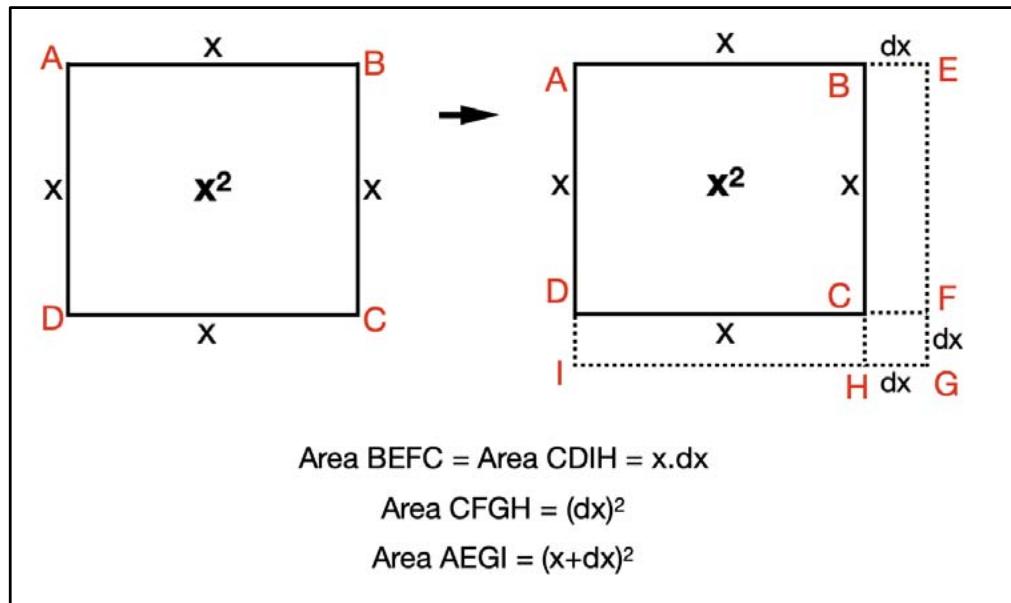Figure 1: The differential small increment in the side of a square from $x$ to $(x + dx)$ So, from equation (10) and (9), one gets, $$ \mathrm{d}y = \left(y_{2}-y_{1}\right) = \left(2x_{1}\mathrm{d}x + \mathrm{d}x^{2}\right) $$ Now, the Newtonian approach was, let $(\mathrm{dx})^2 = 0$ since dx is immeasurably being lower in magnitude, and then, $$ \mathrm{d}y = \left(2\,x_{1}\,\mathrm{d}x\right) \tag{11a} $$ $$ (\mathrm{d}y/\mathrm{d}x) = 2\,x_{1} = 2\,x \text{(generalized)} $$ However, as illustrated in Figure 1, it is observed that when the increment in $\mathbf{x}$ (i.e., $\mathrm{dx}$ ) becomes infinitesimally small, the squared term $\mathbf{x}^2$ essentially begins to regress, and the corresponding change in $\mathbf{y}$ becomes vanishingly small as well. While as per the logic of equation (1), [following equation (11)], $$ \begin{array}{l} \left(\mathrm{d y} / \mathrm{x} _ {1}\right) = \left(2 \mathrm{d x} / \mathrm{x} _ {1}\right) + \left(\mathrm{d x} ^ {2} / \mathrm{x} _ {1}\right) \\= [ 0 + 0 ] \\= 0 \left[ \text{sincedxisinfinitesimallysmall} \right] \tag{13} \\\end{array} $$ According to Newton's approach, the ratio $(\mathrm{dy} / \mathrm{dx})$ -that is, the rate of change of y with respect to x-is meaningful only when x itself is also immeasurably small [3], such that the magnitudes of x and dx are of the same order. As per the topological Diagram (Figure 1), the dy/dx (of Newtonian Calculus) is in fact is being equal to $2\mathrm{x}$ [equation (12)] and hence it is showing the building blocks of the square ABCD since any square is composed of two numbers of straight lines. A square or a rectangle is being formed from the translations of two perpendicular lines through $\mathbf{x}$ and $\mathbf{y}$ axes respectively as is being shown in Figure 1a below.  Figure 1a: The formation of a square from the translations of two numbers of straight lines (the building block of the square) Topologically it is being proved in this article that $(\mathrm{dy} / \mathrm{dx})$ of Newton is basically the 'BUILDING BLOCK ANALYZER' (BBA). As per the Newtonian calculus, $(\mathrm{dy} / \mathrm{dx})$ of $\mathbf{x}^3$ is $3\mathbf{x}^2$ and it will be topologically shown in this article later in this article that a cube is being formed from the translations of 3 numbers of squares in space and hence the 'building block' is 3 numbers of squares of area $\mathbf{x}^2$ each and hence the BBA is $3\mathbf{x}^2$. Consider the second example discussed earlier: let $\mathrm{dx}$ have a magnitude on the order of $10^{-5}$, and suppose that $\mathbf{x}$ also has a similar order of magnitude. In this case, dividing $\mathrm{dy}$ by $\mathrm{dx}$ becomes justifiable, since both variables exist within a microscopic domain—where $\mathrm{dx}$ cannot be considered negligible in comparison to $\mathbf{x}$. Under such conditions, the value of $\mathrm{dy/dx}$, as derived from Equations (11a) and (12), would be: $$ \mathrm{dy} = 2\mathrm{x}_{1}\mathrm{dx} = 2\times10^{-5}\times10^{-5} = 2\times10^{-10} $$ $$ (\mathrm{dy}/\mathrm{dx}) = (2\times10^{-10})/10^{-5} = (2\times10^{-5}) \tag{14} $$ [if $10^{-5}$ is being denoted as for example; p, then dividing $(2\mathrm{x}10^{-10})$ by $10^{-5}$ in equation (14) stands to be dividing $2\mathrm{p}^2$ by p and the numerator i denominator and so it is mathematically being permissible though individually both the numerator and the denominator are small by their magnitudes]. If the value of $x$ be very large say in the order of $10^5$ by its magnitude, then the value of $(\mathrm{dy} / \mathrm{dx})$ would be, as per equation (12), $$ (\mathrm{dy}/\mathrm{dx}) = (2 \times 10^{5} \times 10^{-5} / 10^{-5}) $$ [If $10^{-5}$ is being denoted as for example as; p, then dividing (2) by $10^{-5}$ in equation (15) stands to be dividing 200000p by p (denominator ii numerator) and which does fall in the category of dividing a very large number by a very small number or dividing a number by zero and which is being mathematically non-permissible]. If the Figure 1 is being followed, if $\mathbf{x} = 10^5$, the area of the square shown in Figure 1 would be, $\mathrm{y} = 10^{10}$ and the increased area when $\mathrm{dx} = 10^{-5}$, would be, $$ (1 0 ^ {5} + 1 0 ^ {- 5}) ^ {2} = (1 0 ^ {1 0} + 2 \times 1 0 ^ {5} \times 1 0 ^ {- 5} + 1 0 ^ {- 1 0}) \tag {16} $$ Now, neglecting the last term in equation (16), $$ \text{Increased} = (10^{10} + 2)\tag{17} $$ So, the change in area $= \mathrm{dy} = \left[(\text{final area} - \text{original area}) = [10^{10} + 2 - 10^{10}] = 2 \right.$ (18) As a matter of fact this data 2 [equation (18)] is too negligible compared to the original area of the square, which is $10^{10}$. So at the macroscopic scale the change in area of the square dy is virtually zero. However, compared to the microscopic level, 2 is large but again it faces the mathematically non-permissible operation of dividing 2 by zero since dx is about to be zero. $$ \text {S o}, \quad \left(\mathrm {d y} / \mathrm {d x}\right) = 2 \mathrm {x} 1 0 ^ {5} \tag {19} $$ So, the value of the differential co-efficient does drastically change depending on the value or the magnitude of the variable $\mathbf{x}$, as per Newton's proposition of differential calculus [compare equation (14) and equation (19)]. The principal defects of Newtonian differential calculus are the following: 1. It had not clearly spelt out the range of magnitude of the ratio of $(\mathrm{dx} / \mathrm{x})$, at which the dx should be considered vanishingly small compared to x. 2. The (dy/dx) would be an acceptable version in regard to mathematics only when x and dx both are in the microscopic domain only. 3. The 'differential co-efficient' of Newton's equation is dependent on the magnitude of $x$ itself except when, $y = f(x) = x$. It should ideally be not containing terms retaining $x$. 4. The variable has been considered to be $\mathbf{x}$ only for a relation $y = f(x) = x^n$ (n being any integer). So the variable stands to be $\mathbf{x}$ only whether the function is $\mathbf{x}, \mathbf{x}^2, \mathbf{x}^3, \mathbf{x}^4, \ldots$ and that is also not being true as will be discussed in this article. As a matter of fact, the infinitesimal small change in $\mathbf{x}$, the differential co-efficient in the form of $(\mathrm{dy} / \mathrm{dx})$ is being valid and carries a good physical significance when the co-relation of three numbers of variables are being considered, as for example, if $\mathbf{x}$, $\mathbf{y}$ and $\mathbf{z}$ are three variables inter-related among each other, $$ \text{Let}, \quad \mathrm{y} = (\mathrm{z}). (\mathrm{x}) \tag{20} $$ Now if, to make an infinitesimal small change in the magnitude of $\mathbf{x}$, the magnitude of $\mathbf{z}$ has to change and as a result of that, the magnitude of $\mathbf{y}$ would change. Another model is being required to be developed as an upgradation or the amendment of the differential calculus of Newton, where the division of dy by infinitesimal small amount dx would be avoided and the resulting derivative will not remain related to x. An example of physics will make this subject much clearer. Let, $\mathbf{y} =$ 'energy', $\mathbf{z}$ be the 'force' and $\mathbf{x}$ be the 'distance' in equation (20) and the mathematical relation in physics is, $$ Energy (\mathrm{y}) = Force (\mathrm{z}) \cdot \text{distance} (\mathrm{x}) $$ Let a thin iron wire and a nylon wire of the same cross-sectional thickness be placed side by side. To achieve a unit elongation in the iron wire (from length $x$ to $x + 1$ ), the required force $z$ must be significantly higher than that needed for the nylon wire. In contrast, even a small increase in force $z$ would be sufficient to produce the same unit elongation in the nylon wire. So, (rate of increase of energy /length of the wire) $= (\mathrm{dy} / \mathrm{x}) =$ high for iron wire (rate of increase of energy /length of the wire) $= \left( {\mathrm{{dy}}/\mathrm{x}}\right) =$ low for Nylon wire In such cases the 'differential co-efficient of $y$ with respect to $x$ ' in the form of $\frac{dy}{x}$ of the proposed model would carry a meaningful significance. Let, for the example of the elongation of the wires $$ \text{Initialenergy} \left(\mathrm{y} _ {1}\right) = \text{Force} \left(\mathrm{z} _ {1}\right) \mathrm{x} \text{length} \left(\mathrm{x} _ {1}\right) \tag{22} $$ $$ \text{Finalenergy} \left(\mathrm{y} _ {2}\right) = \text{Force} \left(\mathrm{z} _ {2}\right) \mathrm{x} \text{length} \left(\mathrm{x} _ {2}\right) \tag{23} $$ The change in energy $= \mathrm{dy} =$ change in force (dz) x change in length (dx) $$ Or,\quad \mathrm{dy} = Z_2X_2 - Z_1X_1 $$ Or, $\mathrm{dy} = \mathrm{z}_2(\mathbf{x}_1 + \mathrm{dx}) - \mathrm{z}_1\mathbf{x}_1$ [since $\mathbf{x}_2 = (\mathbf{x}_1 + \mathrm{dx})$, dx is the change in length] Or, $\mathrm{dy} = \mathbf{x}_1\left(\mathbf{z}_2 - \mathbf{z}_1\right) + \mathbf{z}_2\mathrm{dx}$ $$ Or, (dy/x1) = dz + (z2 dx/x1) $$ Or, for dx small, $(\mathrm{dy} / \mathrm{x}1) = \mathrm{dz}$ $$ Or, in general form (dy/x) = dz (24) $$ Another fundamental issue with Newton's model [4] is that, for functions such as $y = f(x) = x$ or $x^2$ or $x^3$ or $x^4 \dots$. the variable is always assumed to be $x$. However, this assumption is not entirely accurate. When the function is simply $x$, the true variable is $x^0$, which represents a dimensionless point. A straight line is being formed by the translation of such points—each of which is, by nature, without dimension. When the function becomes $x^2$ the effective variable is $x$, because over a straight line of fixed length $x$, another straight line begins to grow. This process can be expressed as follows (with $m$ being an integer): $$ \mathrm{y} = \mathrm{f}(\mathrm{x}) = \mathrm{x}(\mathrm{x} + \mathrm{m}\,\mathrm{d}\mathrm{x}) = \mathrm{x}\,\mathrm{x}_{1} [\mathrm{x}_{1} = \mathrm{x} + \mathrm{m}\,\mathrm{d}\mathrm{x}] = \left[\sqrt{\mathrm{x}\,\mathrm{x}_{1}}\right]^{2} = \mathrm{x}_{\mathrm{i}}^{2} (\text{where} \mathrm{x}_{\mathrm{i}} = \left[\sqrt{(\mathrm{x}\,\mathrm{x}_{1})^{1/2}}\right]) $$ Again when the function $y$ is $x^3$, it can be written as, (x remain constant) $$ y = f(x) = x - x^{2} + m(dx)^{2"} = x\,x_{1}^{2}\,[\,x_{1}^{2} = x + m(dx)^{2}\,] = [ (x\,x_{1}^{2})^{1/3} ]^{3} = x_{i}^{3}\,(\text{where}\,x_{i} = [ (x\,x_{1}^{2})^{1/3} ] ) $$ So, the generalized expression would be when $\mathrm{y} = \mathrm{f}(\mathbf{x}) = \mathbf{x}^{\mathrm{n}}$ is $$ \mathrm {y} = \mathrm {f} (\mathrm {x}) = \mathrm {x} ^ {\mathrm {n}} = \mathrm {x} - \mathrm {x} ^ {\mathrm {n} - 1} + \mathrm {m} (\mathrm {d x}) ^ {\mathrm {n} - 1 \prime \prime} = \mathrm {x x} _ {1} ^ {\mathrm {n} - 1} [ \mathrm {x} _ {1} ^ {\mathrm {n} - 1} = \mathrm {x} + \mathrm {m} (\mathrm {d x}) ^ {\mathrm {n} - 1} ] = [ (\mathrm {x x} _ {1} ^ {\mathrm {n} - 1}) ^ {1 / \mathrm {n}} ] ^ {\mathrm {n}} = \mathrm {x} _ {\mathrm {i}} ^ {\mathrm {n}} (\text {w h e r e} \mathrm {x} _ {\mathrm {i}} = [ (\mathrm {x x} _ {1} ^ {\mathrm {n} - 1}) ^ {1 / \mathrm {n}} ] \tag {27} $$ This grow-up of $\mathbf{x}$, $\mathbf{x}^2$, $\mathbf{x}^3$ is shown schematically in Figure 2, Figure 3 and Figure 4 below.  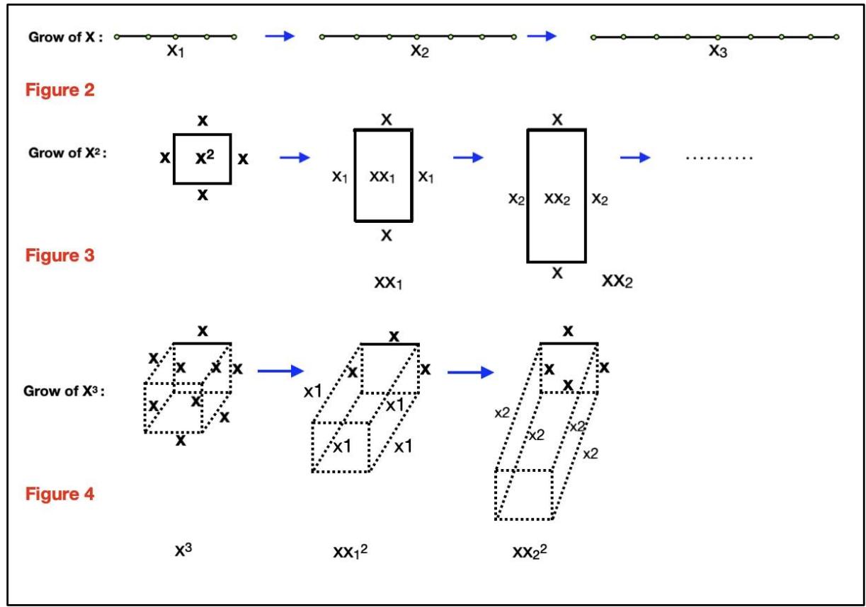Figure 2, 3, 4: Topological presentation of the growth of $\mathbf{xn}$ $(\mathrm{n} = 1,2,3,4\dots)$ So, the conclusion is for any function, in the form of $\mathbf{y} = \mathbf{x}^{\mathrm{n}}$, the variable would be $\mathbf{x}^{(\mathrm{n - 1})}$ only. Now, the derived equation of the dy of a function, $\mathbf{y} = (\mathbf{x}^{\mathrm{n}})$ of Newtonian calculus is, $$ \mathrm{d}y = \mathrm{n}\cdot\mathbf{x}^{n-1}\cdot\mathrm{d}x $$ or, since variable would be $\mathbf{x}^{n - 1}$, following the above said logic and discussions, it can be written, $$ \left(\mathrm{d}y/\mathbf{x}^{n-1}\right) = n\cdot\mathrm{d}x $$ Thus, the rate of change of $y$ with respect to the variable $x^n$ leads to a newly defined differential coefficient, given by $n \cdot dx$. Notably, this expression is independent of the variable itself. In this formulation, the traditional problem of defining the derivative using an infinitesimally small $dx$ approaching zero is effectively avoided. Moreover, the physical significance of this redefined differential coefficient is clearly illustrated through practical examples, such as the variation of energy with respect to displacement or force. Table 1 below presents the differential coefficient of the function $y = x^n$ for various values of $n = 1, 2, 3, 4, 5, \ldots$ Table 1: The newly defined differential co-efficient of $y = {x}^{n}$ for the different values of $n$ <table><tr><td>n</td><td>y=x^n</td><td>(dy/x^{n-1})</td></tr><tr><td>1</td><td>y=x</td><td>(dy/x^0)=1.dx</td></tr><tr><td>2</td><td>y=x^2</td><td>(dy/x)=2.dx</td></tr><tr><td>3</td><td>y=x^3</td><td>(dy/x^2)=3.dx</td></tr><tr><td>4</td><td>y=x^4</td><td>(dy/x^3)=4.dx</td></tr><tr><td>5</td><td>y=x^5</td><td>(dy/x^4)=5.dx</td></tr></table> From Figure 1, it is observed that for the variable x2, two differentials dx are generated. Figure 5, shown below, reveals that for the variable x3, three differentials dx are generated. As the dimensions progress from 1 to 2 to 3 to 4, more and more differentials dx are generated. These concepts are not addressed in Newtonian calculus.   Figure 5: The differential (small) increment of the side $\mathbf{x}$ of a homogeneous cube from $\mathbf{x}$ to $\mathbf{x} + \mathrm{d}\mathbf{x}$, and the associated change in the volume of the cube ## II. THE NEW CONCEPT OF INTEGRATION OF VARIABLES IN THE FORM OF $X^{\mathbb{N}}$ It can be observed from Figure 1 and Figure 5 that, in the expanded form of $(\mathrm{x + dx})$, the topologies for x2 and x3 emerge in their differential forms. If these differential forms of the respective functions are folded back, the original functions x2 and x3 are recovered. Thus, the integrated forms are the original functions themselves, obtained by folding back the expanded (or differential) expressions. Now for the function $$ x^{2},\,\mathrm{d}y\left(x^{2}\right) = 2x.\mathrm{d}x + \mathrm{d}x^{2} $$ Neglecting, the term $\mathrm{dx}2$, one gets, $\mathrm{dy}(\mathbf{x}^2) = 2\mathbf{x}.\mathrm{dx}$ (31) So, as follows from equation (31), $\int 2\mathbf{x} \, \mathrm{d}\mathbf{x} = \mathbf{x}^2 + \mathbf{I}$ (32) Or, $\int \mathbf{x} \, \mathrm{d}\mathbf{x} = \left( \frac{\mathbf{x}^2}{2} \right) + \mathbf{I}$ (33) Parameter I is a constant of integration, and its physical significance will be discussed later in this article. For now, the discussion will proceed with the understanding that this constant of integration is acknowledged. For the function $y = x^3$, it can be written, $$ \mathrm {d y} \left(\mathrm {x} ^ {3}\right) = 3 \mathrm {x} ^ {2} \mathrm {d x} + 3 \mathrm {x} \mathrm {d x} ^ {2} \tag {34} $$ Neglecting dx2 term in equation (34), one obtains, $$ \mathrm{d}y\left(\mathrm{x}^{3}\right) = 3\mathrm{x}^{2}\mathrm{d}x \tag{35} $$ and hence, $\int 3\mathbf{x}^2\mathrm{d}\mathbf{x} = \mathbf{x}^3$ (36) or, $\int \mathrm{x}^2\mathrm{d}\mathrm{x} = (\mathrm{x}^3 /3)$ (37) So here, in a very straightforward manner, the concept of integration is being elaborated. In contrast, Newton's derivation of the integral of $\mathbf{x}^{\mathrm{n}}$ is not only cumbersome but also flawed, as it introduces an integral of the form [1. dx] without providing a clear physical interpretation. The meaning and justification of this integral remain unexplained. At its core, both differentiation and integration originate from spatial concepts—a point that will now be further explored. It becomes easier to explain these spatial foundations of calculus when one begins with the process of integration. In Figure 6 below, it is illustrated how integration is directly related to the translation of variables in space.  Figure 6: The concept of integration of variables in regard to translation and rotation In Figure 6, it is shown that a line segment of length $x$ moves through space: beginning in one dimension, it extends into a second dimension and generates an area of $x^2 / 2$ in the form of a square. This square then moves through space into a third dimension, forming a cube with a volume of $x^3 / 3$. In the same figure, it is also shown that a straight line of length $r$ rotates in a plane (i.e., in two-dimensional space), generating a circle of area $\pi r^2 / 2$. When this circle rotates around its axis, a sphere is formed, with a volume of $(1/3 \times 4\pi r^3 / 3)$. Thus, integration can be understood as the process of spatial hybridization of variables—through either translation or rotation. Dimensionally, integrating $\mathbf{x}$ gives rise to $\mathbf{x}^2$ and further integration of $\mathbf{x}^2$ yields $\mathbf{x}^3$, as is also known from Newton's standard integral calculus formula: $$ \int \mathrm{x}^{\mathrm{n}} \, \mathrm{d x} = \left(\mathrm{x}^{\mathrm{n + 1}} / \mathrm{n + 1}\right) \tag{38} $$ As per Equation (38), the integrals of $\mathbf{x}$ and $\mathbf{x}^2$ are $\mathbf{x}^2 / 2$ and $\mathbf{x}^3 / 3$, respectively. However, in Figure 6, the result of spatial integration shows that a factor of 2 appears in the integration of $\mathbf{x}$. This occurs because the translation of a straight line segment of length $\mathbf{x}$ along the $\mathbf{x}$ -axis produces an area of $(\mathbf{x}^2 / 2)$, and a similar translation of the same segment along the $\mathbf{y}$ -axis generates an additional area of $(\mathbf{x}^2 / 2)$. Together, these form the full area of the square ABCD, equal to $\mathbf{x}^2$. This is illustrated clearly in Figure 7 below.  Figure 7: Topology of formation of a square in space In Figure 6, it is shown that when a straight line of length (or radius) $r$ rotates about the $x$ -axis, it generates an area of $\pi r^2 / 2$. When the same line rotates about the $y$ -axis, it produces another area of $\pi r^2 / 2$. The sum of these two areas yields the total area of a full circle, $\pi r^2$. Similarly, in the same figure, the translation of a square with area $x^2$ along the $x-$, $y-$, and $z$ -axes generates volumes of $x^3 / 3$ for each direction. The total volume formed by these three translations equals $x^3$. Additionally, when a circle of area $\pi r^2$ undergoes rotation about the $x-$, $y-$, and $z$ -axes, each rotation results in the formation of a spherical volume of $(1 / 3 x 4\pi r^3 / 3)$. The combined volume of the three such spheres adds up to $(4\pi r^3 / 3)$, which corresponds to the known volume of a full sphere. The following important points are to be noted: 1. A square (of length of each side, $\mathbf{x}$ ) does contain 2 numbers of inner squares of area each $(\mathbf{x}^2 / 2)$. 2. A cube (of length of each side, $\mathbf{x}$ ) does contain 3 numbers of inner cubes of volume each $(\mathrm{x}^3 / 3)$. 3. A circle (of radius, r) does contain 2 numbers of inner circles of area each $(\pi r^2 /2)$. 4. A sphere (of radius, r) does contain 3 numbers of inner spheres of volume each $(1/3 \times 4\pi r^3/3)$. The process of differentiation is essentially the reverse of integration. In differentiation, the integrated variables undergo de-hybridization—they isolate themselves from the spatial continuity or integrity established during integration. This concept is illustrated in Figure 8 below.     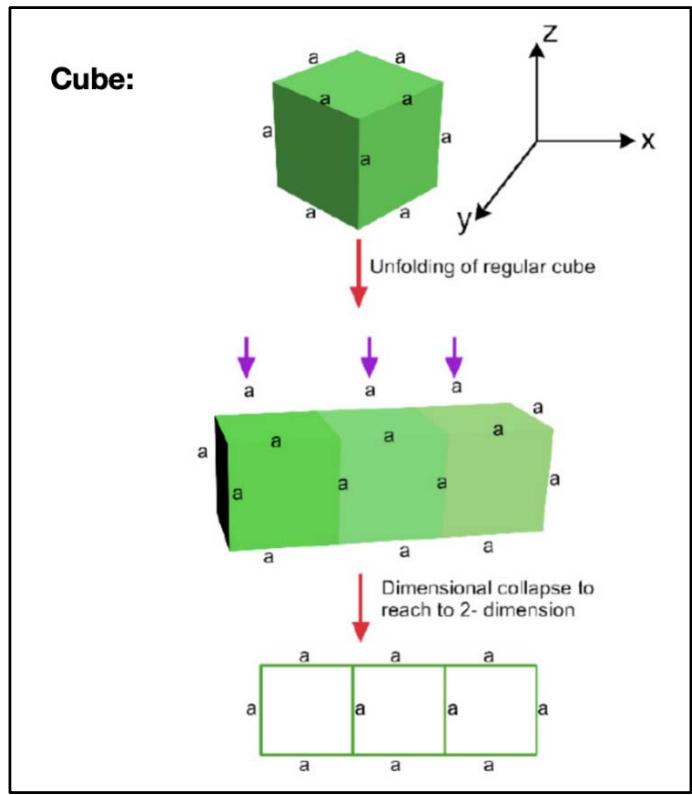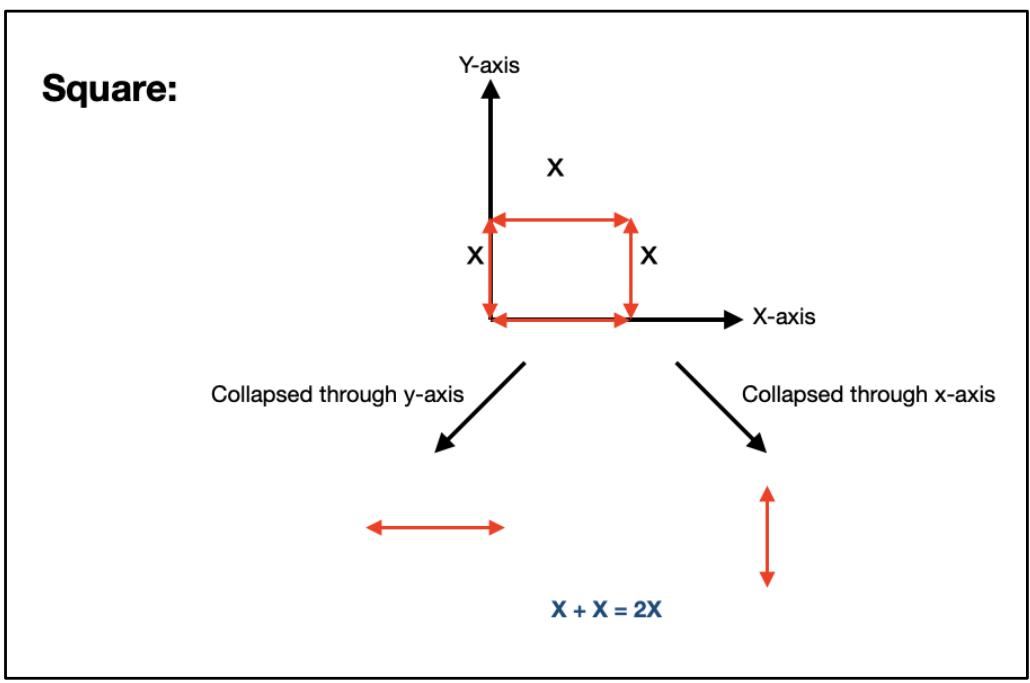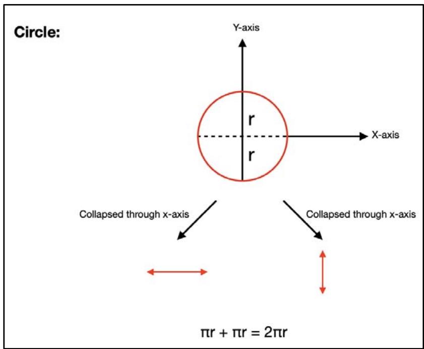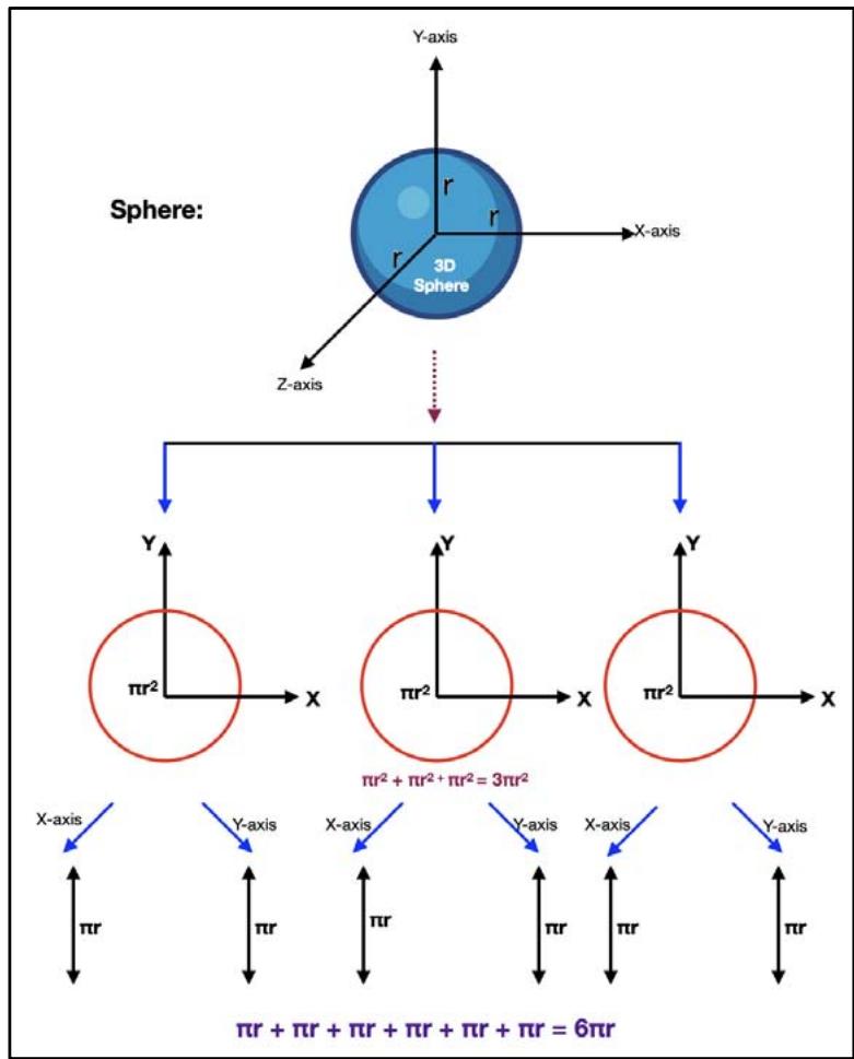Figure 8: Topological cum dimensional degradation of the process of so called differentiation of Newtonian Calculus (being redefined as BBA in this research article) In figure 8, it is being shown that a cube of volume $\mathbf{x}^3$ do collapses back to 3 numbers of squares each along $\mathbf{x}$, $\mathbf{y}$ and $\mathbf{z}$ axis respectively and the area of each square becomes $\mathbf{x}^2$ and hence, $$ Building Block of \mathbf{x}^3 = \left(\mathbf{x}^2 + \mathbf{x}^2 + \mathbf{x}^2\right) = 3\mathbf{x}^2 $$ $$ \text{BuildingBlock} \quad \mathrm{x}^2 = (\mathrm{x} + \mathrm{x}) = 2\mathrm{x} \tag{40} $$ $$ \text{BuildingBlock} (\pi \mathrm{r}^2) = (\pi \mathrm{r} + \pi \mathrm{r}) = 2 \pi \mathrm{r} $$ $$ \text{Building} \left(4\pi r^{3}/3\right) = \left(\pi r^{2} + \pi r^{2} + \pi r^{2}\right) = 3\pi r^{2} \tag{42} $$ In figure 8, it is shown that the parameter $3\pi r^2$ does collapse back to 6 numbers of length $\pi r$, 2 numbers of $\pi r$ each along $x$, $y$ and $z$ axes respectively. $$ \text{BuildingBlock} \left(3\pi r^{2}\right) = \left(\pi r + \pi r + \pi r + \pi r + \pi r + \pi r\right) = 6\pi r \tag{43} $$ From this model, one can begin to understand the physical significance of the universal constant $\pi$. Geometrically, the expression $\pi r$ represents a half-circle. When two such half-circles face each other and unite, they form a complete circle. As illustrated in Figure 9, when this circle is uniformly compressed from all directions in space, it collapses—the radius $r$ reduces to a unit length, which is proposed as the smallest possible length in the universe. A new circle is then formed with this minimal radius. Thus, $\pi$ can be interpreted as representing the smallest possible volumetric unit of space—a fundamental quantum of geometry. These $\pi$ based units exist only in space, and they act as the foundational building blocks of other space quanta associated with force, energy, electromagnetic waves, and more.  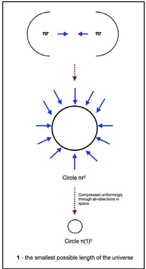Figure 9: Generation $\pi$ space quantum of the universe Now the origin of the constant of integration I, of indefinite integrals would be explained. In figure 10 below it is being shown, as a straight line of segment length L, as for example, translates in space in 2-dimension, and it can translate to even infinity (crossing the length L) or might be translating to a distance which is less than L as being shown in Figure 10.  Figure 10: Topological presentation of "Integration Constant" When it translates up to a distance $L$ only, the value of the integration is $(L^2 / 2)$. So when it translates beyond the length $L$, the result of integration is, $$ \text{Integration} \mathrm{L} = \left(\mathrm{L} ^ {2} / 2\right) + \mathrm{I} (\mathrm{I} = + \mathrm{v e}) \tag{44} $$ When the line translates to any length which is lesser than L, $$ \text{Integration} \mathrm{L} = \left(\mathrm{L}^{2}/2\right) + \mathrm{I} \left(\mathrm{I} = -\mathrm{ve}\right) \tag{45} $$ The above discussions truly reveal the physical significance of the constant of integration $\mathrm{T}'$. ## III. DERIVATIVES AND INTEGRATIONS OF THE TRIGONOMETRIC FUNCTIONS In trigonometry the trigonometric variables are $\sin\theta$, $\cos\theta$, $\tan\theta$, $\cot\theta$, $\sec\theta$ and $\csc\theta$ respectively where $\theta$ is the angle opposite to the perpendicular of a right-angled triangle. One important point to note in trigonometry is, these are not valid for 1 dimension since in 1 dimension a triangle cannot be constructed. So the dimension should be at least 2 or 3 dimensions. The values of the above trigonometric functions are principally being expressed at 0, 30, 45, 60 and 90 degree angles in the subject of trigonometry. As shown in Figure 10a below, as the value of $\theta$ becomes zero or 90 degree, the dimension becomes 1 dimension only and the entire subject of trigonometry does not stand in regard to physics although they might be mathematically valid. 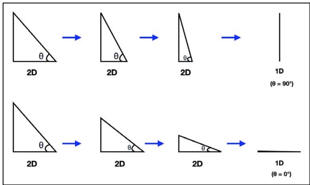So the limit theorems of Newtonian calculus are not being the valid or justified ones,  Figure 10a: The Dimensional degradation of a triangle at $\theta = 0$ and $90\mathrm{fl}$ respectively The conventional unit circle concept of trigonometry is based on a circle of radius unity as shown in Figure 10b and the x and y co-ordinates of any point P (on the circumference of the circle) are being considered to be $\cos\theta$ and $\sin\theta$ respectively. The radius OP makes an angle $\theta$ at the point of origin. However, when the radius OP as is being shown in Figure 10a, falls on the x axes the angle $\theta$ is being zero and the length OP $= 1$, on x axes and since $\cos 0 = 1$, the x co-ordinate of point P is considered to be $\cos \theta$. However, when the radius OP falls on the y axes, $\theta$ is 90 degree and the length of OP on y axes is unity too and since $\sin 90 = 1$, the co-ordinate of point P on y axes is considered to be $\sin \theta$.  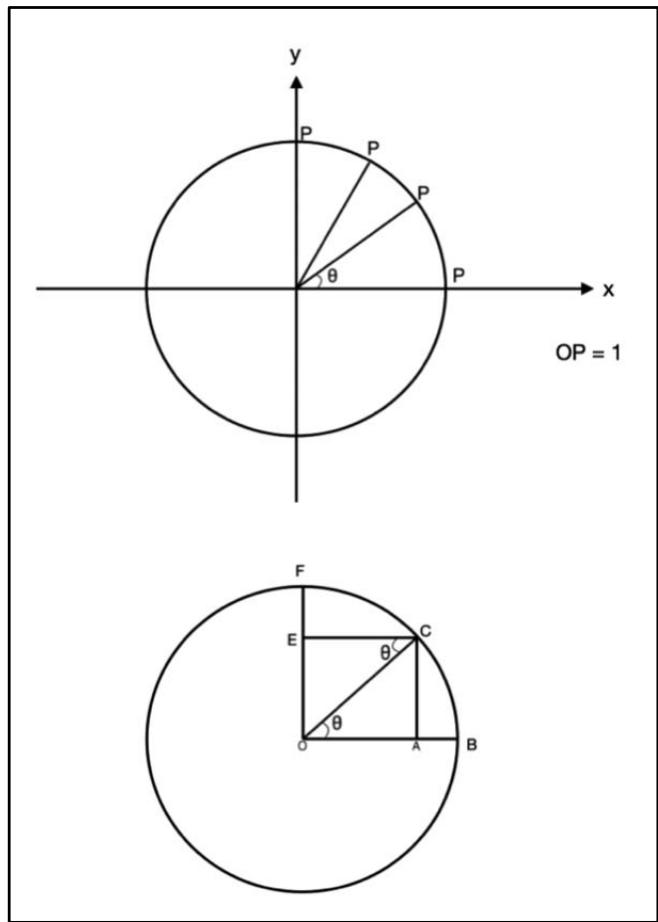Figure 10b: Latent triangle concept of trigonometry in the unit circle concept This unit circle concept of trigonometry is being fundamentally based on triangle concept since as being shown in Figure 10b, in triangle AOC, $$ \begin{array}{r l} \operatorname{Sin} \theta = (\mathrm{A C} / \mathrm{O C}) & = (\mathrm{O E} / \mathrm{O C}) \end{array} \tag{45a} $$ In triangle EOC, $\mathrm{Cos}\theta = (\mathrm{EC} / \mathrm{OC}) = (\mathrm{OA} / \mathrm{OC})$ (45b) Now since $\mathrm{OC} =$ radius of the circle $= 1$, then, $$ \sin\theta = \mathrm{OE} = \text{x co-ordinate of point P} $$ and $\mathrm{Cos}\theta = \mathrm{OA} = \mathrm{y}$ co-ordinate of point P (45d) The triangle concept of trigonometry is being latent in the unit circle concept of the same. The unit circle concept is being evolved from the triangular concept of trigonometry as is being presented here and which is not applicable at 0 and 90 degree angles as has been already discussed earlier. The derivatives of the trigonometric functions like $\mathrm{d} / \mathrm{d}\theta$ ( $\sin\theta$ ), $\mathrm{d} / \mathrm{d}\theta$ ( $\cos\theta$ ), $\mathrm{d} / \mathrm{d}\theta$ ( $\tan\theta$ ) [where the trigonometric variables are being the y variable and $\theta$ the x variable] as evaluated by Newton are valid in the range when the magnitudes of $\mathrm{d}\theta$ and the trigonometric functions ( $\sin\theta$, $\cos\theta$, $\tan\theta$ ) are being comparable. As per Newton's derivation of the derivatives of the trigonometric functions, $$ \mathrm {d} / \mathrm {d} \theta (\sin \theta) = \cos \theta \tag {46} $$ $$ \mathrm{d}/\mathrm{d}\theta \left(\cos \theta\right) = -\sin \theta \tag{47} $$ $$ \mathrm{d}/\mathrm{d}\theta\left(\tan\theta\right) = \sec^{2}\theta \tag{48} $$ $$ \mathrm {d} / \mathrm {d} \theta (\cot \theta) = - \sec^ {2} \theta \tag {49} $$ $$ \mathrm{d}/\mathrm{d}\theta\left(\sec\theta\right) = \sec\theta\tan\theta $$ $$ \mathrm{d}/\mathrm{d}\theta\left(\operatorname{cosec}\theta\right) = -\operatorname{cosec}\theta\cot\theta \tag{51} $$ The above said derivations of Newton are fully mathematical without involving the geometrical aspects and in fact are falsified too since they are based on so many assumptions and limit theorems. A new geometric or topological model will be presented in this article for determining the derivatives [in the form of $\mathrm{d}(\sin \theta) / \theta$, $\mathrm{d}(\cos \theta) / \theta$, etc] of the trigonometric functions. The following points to note in this regard: 1. At first all the equations (46) to (51) of Newton's will be derived through the said new model 2. The flaws of the concepts of Newton will be shown 3. Finally, the actual derivatives of all the trigonometric derivatives will be derived through this new model. 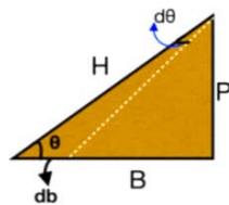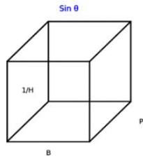As being shown in Figure 11 below, the perpendicular (P), the base (B) and the hypotenuse (H) makes a cuboid (In all the geometries of the cuboids of Figure 11, the lengths of the perpendicular, base and the hypotenuse is taken to be, $\mathrm{P} = 1$, $\mathrm{B} = 1$ and $\mathrm{H} = \sqrt{2}$, as per Pythagoras theorem). For the different trigonometric functions, as shown below mathematically (also geometrically in Figure 11) the shapes or the volumes of the cuboid do differ among each other of the trigonometric functions. For each of the trigonometric functions out of the three numbers (P, B & H) of sides of the cuboid, one of the sides go to the inverse dimensions, as shown below, in Table 2 below. In regard to a right angled triangle as the length of perpendicular increases by an infinitesimal small length, dP, the angle $\theta$, would also increase by dθ, as is shown in Figure 11 below. It is to note that dθ would be proportional to dP. On the other hand when the base of the said right angled triangle decreases by an infinitesimal small magnitude dB, the angle $\theta$ does increase too and in that case, dθ would be proportional to dB.    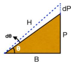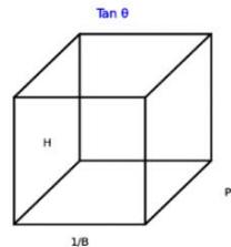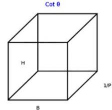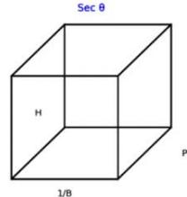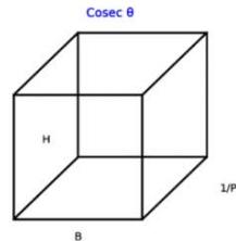Unit Cuboid Concept:      Figure 11: Diagrammatic presentation of the different cuboids belonging to $\sin\theta$, $\cos\theta$, $\tan\theta$, $\cot\theta$, $\sec\theta$ and $\csc\theta$ Table 2: The different shapes of the trigonometric functions and their changes when the angle $\theta$ increases by infinitesimal amount $d\theta$ <table><tr><td>(secθ)</td><td>(H/B)</td><td>P, (1/B), H</td><td>(PH/B)</td><td>[P H/(B-dB)]</td><td>[P H/(B-dB)] - (PH/B) = [PHdB/(B2-BdB)] = [PHdB/B2] B2&gt;&gt; BdB So BdB neglected in the denominator</td><td>B decreases, P remain constant and decrease in B leads to increase in θ [since secθ = H/B]</td></tr><tr><td>(cosecθ)</td><td>(H/P)</td><td>H, (1/P), B</td><td>(HB/P)</td><td>[(HB/(P +dP)]</td><td>[(HB/(P +dP)] - (HB/P) = [-HBdP/ (P2 +PdP)] = -[HBdP/P2] Since P2&gt;&gt;PdP PdP being neglected in the denominator</td><td>B remains constant and increase in P leads to increase in θ [since Cosecθ = H/P]</td></tr></table> <table><tr><td>Trigonomet ric Function</td><td>The definition of the trigonometric functions in regard to P,B &amp; H</td><td>The 3 numbers of sides of the cuboid</td><td>Initial volume of the cuboid Vi</td><td>Final volume of the cuboid when θ increases by dθ \({\mathrm{V}}_{\mathrm{f}} \)</td><td>Change in the volume of the cuboid \(\Delta \mathrm{V} = \left({{\mathrm{V}}_{\mathrm{f}} - {\mathrm{V}}_{\mathrm{i}}}\right) \)</td><td>Consequence</td></tr><tr><td>(sinθ)</td><td>(P/H)</td><td>P, (1/H), B</td><td>(PB/H)</td><td>\(\left\lbrack {\left({\mathrm{P} + \mathrm{{dP}}}\right) \mathrm{B}/\mathrm{H}}\right\rbrack \)</td><td>[BdP/H]</td><td>B remains constant and increase in P leads to increase in θ [since sinθ =P/H, increase in P is considered]</td></tr><tr><td>(cosθ)</td><td>(B/H)</td><td>P, (1/H), B</td><td>(PB/H)</td><td>\(\left\lbrack {\left({\mathrm{P}\left({\mathrm{B} - \mathrm{{dB}}/\mathrm{H}}\right)}\right\rbrack}\right\rbrack \)</td><td>-[PdB/H]</td><td>P remains constant and decrease in B leads to increase in θ [since cosθ =B/H, decrease in B is being considered</td></tr><tr><td>(tanθ)</td><td>(P/B)</td><td>P, (1/B), H</td><td>(PH/B)</td><td>\(\left\lbrack {\left({\mathrm{P} + \mathrm{{dP}}}\right) \mathrm{H}/\mathrm{B}}\right\rbrack \)</td><td>[BdP/H]</td><td>B remains constant and increase in P leads to increase in θ [since tanθ =P/B, increase in P is being considered]</td></tr><tr><td>(cotθ)</td><td>(B/P)</td><td>B, (1/P), H</td><td>(HB/P)</td><td>\(\left\lbrack {\left({\mathrm{B} - \mathrm{{dB}}}\right) \mathrm{H}/\mathrm{P}}\right\rbrack \)</td><td>-[HdB/P]</td><td>P remains constant and decrease in B leads to increase in θ [since cot \(\theta = \mathrm{B}/\mathrm{P} \), decrease in B is being considered</td></tr></table> For deriving the differential co-efficient of the trigonometric functions by Newton, some or the other limit theorems, the reciprocal formula and the chain rule in calculus was used by Newton. However, without using any such approximation, the derivatives of the trigonometric functions will be derived. For $\mathrm{Sin}\theta$, as per Table 2, Difference in volume of the cuboid $= \mathrm{dy} = \mathrm{d}$ $(\sin \theta) = [\mathrm{BdP / H}]$ $$ \mathrm{Or},\quad = \cos\theta\,\mathrm{d}P $$ $$ \text{O r}, \quad = \cos \theta \mathrm{d} \theta [ \text{since} \cos \theta = (\mathrm{B} / \mathrm{H}) \text{and} \mathrm{d P} = \mathrm{d} \theta \text{inregardtolength} ] \tag{52} $$ For $\mathrm{Cos}\theta$, as per Table 2, Difference in volume of the cuboid $= \mathrm{dy} = \mathrm{d}$ $(\cos \theta) = -[\mathrm{PdB / H}]$ $$ \mathrm{Or},\quad = - \sin\theta\,\mathrm{d}B $$ $$ \text{O r}, \quad = - \sin \theta \mathrm{d} \theta \quad [ \text{since} \sin \theta = (\mathrm{P} / \mathrm{H}) \text{and} \mathrm{d B} = \mathrm{d} \theta \text{inregardtolength} ] \tag{53} $$ Fortan,asperTable2 Difference in volume of the cuboid $= \mathrm{dy} = \mathrm{d}\left( {\tan \theta }\right) = \left\lbrack {\mathrm{{BdP}}/\mathrm{H}}\right\rbrack$ $$ Or, = \sec\theta\,\mathrm{d}B $$ $$ \operatorname{O r}, = \sec \theta \mathrm{d} \theta [ \text{since} \sec \theta = (\mathrm{B} / \mathrm{H}) \text{and} \mathrm{d B} = \mathrm{d} \theta \text{inregardtolength} ] \tag{54} $$ For cotθ, as per Table 2, Difference in volume of the cuboid $= \mathrm{dy} = \mathrm{d}(\tan \theta) = -[\mathrm{HdB / P}]$ $$ \mathrm{O r}, = - \text{Cosec} \theta \mathrm{d B} $$ $$ \text{O r}, = - \operatorname{Cosec} \theta \mathrm{d} \theta [ \text{sinceCosec} \theta = (\mathrm{H} / \mathrm{P}) \text{and} \mathrm{d B} = \mathrm{d} \theta \text{inregardtolength} ] \tag{55} $$ For $\operatorname{Sec}\theta$, as per Table 2, Difference in volume of the cuboid $= \mathrm{dy} = \mathrm{d}\left(\tan \theta\right) = \left[\mathrm{PHdB} / \mathrm{B}^{2}\right]$ $$ = \left[ (\mathrm {H} / \mathrm {B}) \mathrm {x} (\mathrm {P} / \mathrm {B}) \right] \mathrm {d B} $$ $$ = \operatorname{Sec} \theta \operatorname{Tan} \theta \mathrm{d} \theta $$ $$ \text{O r}, \quad = \operatorname{Sec} \theta \operatorname{Tan} \theta \mathrm{d} \theta [ \text{since} \operatorname{Tan} \theta = (\mathrm{P} / \mathrm{B}) \text{and} \mathrm{d B} = \mathrm{d} \theta \text{inregardtolength} ] \tag{56} $$ For Cosecθ, as per Table 2, $$ \begin{array}{l} \text{Difference in volume of the cuboid} = \mathrm{d} (\operatorname{Cosec} \theta) = - [\mathrm{H B d P / P^{2}}] \\= - [ (\mathrm{H}/\mathrm{B}) \times (\mathrm{B}/\mathrm{P}) ] \, \mathrm{d} \mathrm{P} \end{array} $$ $$ \mathrm {O r}, \quad = - \operatorname {C o s e c} \theta \cot \theta \mathrm {d B} $$ $$ \text {O r}, \quad = - \operatorname {C o s e c} \theta \cot \theta d \theta [ \text {s i n c e C o s e c} \theta = (\mathrm {H} / \mathrm {P}) \text {a n d} \mathrm {d B} = \mathrm {d} \theta \text {i n r e g a r d t o l e n g t h} ] \tag {57} $$ Table 3 below shows the results of derivation of the derivatives of the trigonometric functions as per the model of this article vis-à-vis Newton's findings. Table 3: The derivatives of the trigonometric functions, Newton vis-à-vis model of this article <table><tr><td>Trigonometric function</td><td>Expression of derivative of Newton model</td><td>Newton&#x27;s results</td><td>Expression of derivative of new model</td><td>New model results</td></tr><tr><td>Sinθ</td><td>d/dθ (sinθ)</td><td>Cosθ</td><td>d(sinθ)/θ</td><td>Cosθdθ/θ</td></tr><tr><td>Cosθ</td><td>d/dθ (cosθ)</td><td>-Sinθ</td><td>d(cosθ)/θ</td><td>-Sinθdθ/θ</td></tr><tr><td>Tanθ</td><td>d/dθ (Tanθ)</td><td>Sec2θ</td><td>d(tanθ)/θ</td><td>Secθdθ/θ</td></tr><tr><td>Cotθ</td><td>d/dθ (cotθ)</td><td>-Cosec2θ</td><td>d(cotθ)/θ</td><td>-Cosecθdθ/θ</td></tr><tr><td>Secθ</td><td>d/dθ (secθ)</td><td>Secθ Tanθ</td><td>d(secθ)/θ</td><td>SecθTanθdθ/θ</td></tr><tr><td>Cosecθ</td><td>d/dθ (Cosecθ)</td><td>-cosecθ cotθ</td><td>d(Cosecθ)/θ</td><td>-cosecθcotθdθ/θ</td></tr></table> The results of the expressions of the trigonometric derivatives do match for sin, cosine, sec and cosec functions for the Newton's model vis-a-vis the current model as is being found from the above Table 3. However, the results do differ for tan and cot functions. While the model of Newton is a pure mathematical model and for deriving the derivatives of tan and cot functions he used product rule, chain rule and quotient rule of the differential calculus but for the other trigonometric functions (sine, cosine, sec and cosec functions) the said rules were not being utilized. So this raises the question of validity of the said rules. The model presented in this article is a tripartite model in regard to mathematics, geometry and physics and the derivations are very straight forward and the students of mathematics would find the proposed model very simple and easily understandable. The concept of physics is utilized for $\theta$ values 0 and 90 degree since at the said values the trigonometric functions have no validity since the dimension converges to one dimension. So, the derived results for the current model stand justified compared to Newton's model. Table 4: Sinθ to θ data of literature for θ = 10, 20, 30, 40, 50, 60, 70, 80 <table><tr><td>θ</td><td>Sinθ</td><td>Δ sinθ</td><td>Δ sinθ/θ</td><td>Δθ</td><td>(Δ sinθ/Δθ)</td><td>Cos θ</td></tr><tr><td>10</td><td>0.173</td><td>-</td><td></td><td></td><td></td><td>0.984</td></tr><tr><td>20</td><td>0.342</td><td>0.169</td><td>0.0169</td><td>10</td><td>0.00169</td><td>0.940</td></tr><tr><td>30</td><td>0.500</td><td>0.327</td><td>0.0327</td><td>20</td><td>0.01635</td><td>0.866</td></tr><tr><td>40</td><td>0.643</td><td>0.47</td><td>0.0470</td><td>30</td><td>0.01566</td><td>0.766</td></tr><tr><td>50</td><td>0.766</td><td>0.593</td><td>0.0593</td><td>40</td><td>0.01482</td><td>0.643</td></tr><tr><td>60</td><td>0.866</td><td>0.693</td><td>0.0693</td><td>50</td><td>0.01386</td><td>0.500</td></tr><tr><td>70</td><td>0.940</td><td>0.767</td><td>0.0767</td><td>60</td><td>0.01278</td><td>0.340</td></tr><tr><td>80</td><td>0.984</td><td>0.811</td><td>0.0811</td><td>70</td><td>0.01158</td><td>0.170</td></tr></table> Table 5: Cosθ to θ data of literature for θ = 10, 20, 30, 40, 50, 60, 70, 80 <table><tr><td>θ</td><td>Cosθ</td><td>Δ Cosθ</td><td>Δ cosθ/θ</td><td>Δθ</td><td>(Δ cosθ/Δθ)</td><td>-sinθ</td></tr><tr><td>10</td><td>0.9848</td><td>-</td><td></td><td></td><td></td><td>-0.1736</td></tr><tr><td>20</td><td>0..9396</td><td>-0.0452</td><td>-0.00452</td><td>10</td><td>-0.00452</td><td>-0.3420</td></tr><tr><td>30</td><td>0..8660</td><td>-0.1188</td><td>-0.01188</td><td>20</td><td>-0.00594</td><td>-0.5000</td></tr><tr><td>40</td><td>0.7660</td><td>-0.2188</td><td>-0.02188</td><td>30</td><td>-0.00729</td><td>-0.6427</td></tr><tr><td>50</td><td>0.6427</td><td>-0.3421</td><td>-0.03421</td><td>40</td><td>-0.00855</td><td>-0.7660</td></tr><tr><td>60</td><td>0.5000</td><td>-0.4840</td><td>-0.04840</td><td>50</td><td>-0.00968</td><td>-0..8660</td></tr><tr><td>70</td><td>0.3420</td><td>-0.6428</td><td>-0.06428</td><td>60</td><td>-0.10710</td><td>-0.9396</td></tr><tr><td>80</td><td>0.1736</td><td>-0.8112</td><td>-0.08112</td><td>70</td><td>-0.01158</td><td>-0.9848</td></tr></table> Table 6: Tanθ to θ data of literature for θ = 10, 20, 30, 40, 50, 60, 70, 80 <table><tr><td>θ</td><td>Tanθ</td><td>Δ tanθ</td><td>Δ tanθ/θ</td><td>Δθ</td><td>(Δ tanθ/Δθ)</td><td>secθ</td><td>Sec2θ</td></tr><tr><td>10</td><td>0.176</td><td>-</td><td></td><td></td><td></td><td>1.010</td><td>1.02</td></tr><tr><td>20</td><td>0.363</td><td>0.187</td><td>0.0187</td><td>10</td><td>0.00187</td><td>1.064</td><td>1.13</td></tr><tr><td>30</td><td>0.577</td><td>0.401</td><td>0.0401</td><td>20</td><td>0.02005</td><td>1.154</td><td>1.32</td></tr><tr><td>40</td><td>0.839</td><td>0.663</td><td>0.0663</td><td>30</td><td>0.02210</td><td>1.305</td><td>1.70</td></tr><tr><td>50</td><td>1.191</td><td>1.015</td><td>0.1015</td><td>40</td><td>0.02525</td><td>1.555</td><td>2.41</td></tr><tr><td>60</td><td>1.732</td><td>1.556</td><td>0.1556</td><td>50</td><td>0.03112</td><td>2.000</td><td>4.00</td></tr><tr><td>70</td><td>2.747</td><td>2.571</td><td>0.2571</td><td>60</td><td>0.04285</td><td>2.923</td><td>8.54</td></tr><tr><td>80</td><td>5.671</td><td>5.495</td><td>0.5495</td><td>70</td><td>0.0785</td><td>5.758</td><td>33.15</td></tr></table> The plots of $(\Delta \sin \theta / \Delta \theta)$ versus $\theta$, $(\Delta \sin \theta / \theta)$ versus $\theta$ and $\cos \theta$ versus $\theta$ are being shown in Figure 12 below:  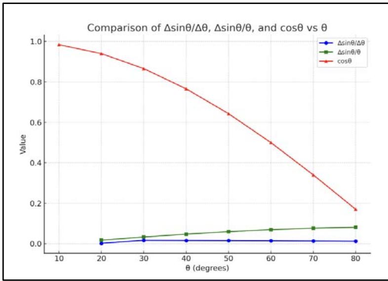Figure 12: Plot of data of Table 4 The plots of $(\Delta \cos \theta / \Delta \theta)$ versus $\theta$, $(\Delta \cos \theta / \theta)$ versus $\theta$ and $-\sin \theta$ versus $\theta$ are being shown in Figure 13 below:  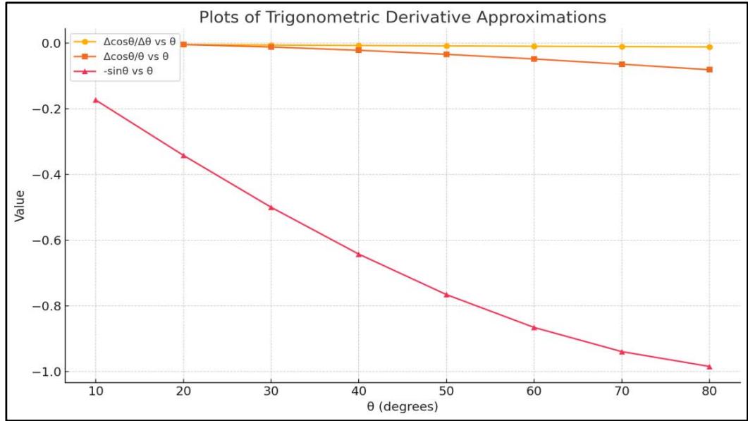Figure 13: Plot of Data of Table 5 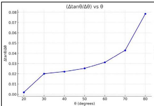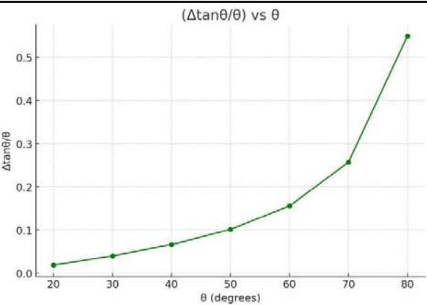The plots of $(\Delta \tan \theta / \Delta \theta)$ versus $\theta$, $(\Delta \tan \theta / \theta)$ versus $\theta$, $\sec \theta$ versus $\theta$ and $\sec 2\theta$ versus $\theta$ are being shown in Figure 14 below:    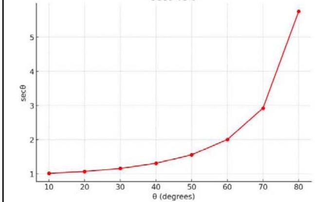secθ vs θ  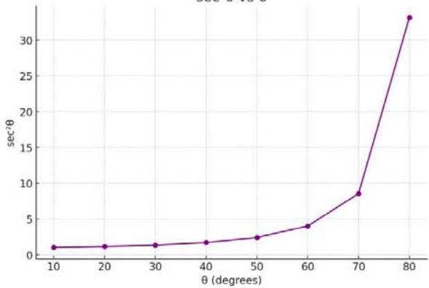Figure 14: Plot of data of Table 6 Now the results of integration of the trigonometric functions would just be the reverse of the differentiation, as for example, (to note Table 3). $$ \mathrm {d} (\sin \theta / \theta) = \cos \theta $$ So, $\int \cos \theta \mathrm{d}\theta = \sin \theta$ (57a) $$ \int \sin \theta d \theta = - \cos \theta \tag {57b} $$ $$ \int \sec \theta \tan \theta \mathrm {d} \theta = \sec \theta \tag {57c} $$ $$ \int \operatorname {c o s e c} \theta \cot \theta d \theta = - \operatorname {c o s e c} \theta \tag {57d} $$ $$ \int \sec \theta d \theta = \tan \theta \tag {57e} $$ $$ \int \operatorname {c o s e c} \theta \mathrm {d} \theta = - \cot \theta \tag {57f} $$ Proposed new model of deriving the integration of trigonometric functions The new proposed model would be similar to the proposed model of finding the differential coefficients as presented in the previous section. As has been shown in the previous section both topologically and mathematically that the differential form of a function, if being integrated, the original function is being retained back. $$ \int 2 x d x = x ^ {2} $$ So to obtain the integration results of a trigonometric function, as for example, $\sin \theta$, a function has to be found out, the differential form which is being $\sin \theta$. Then the said searched or found out function would be the result of integration of $\sin \theta$. To make this very clearly understandable, the Table 2 is being reproduced below, Table 2: The different shapes of the trigonometric functions and their changes when the angle $\theta$ increases by infinitesimal amount $d\theta$ <table><tr><td>Trigonometric Function</td><td>The definition of the trigonometric functions in regard to P,B &amp; H</td><td>The 3 numbers of sides of the cuboid</td><td>Initial volume of the cuboid Vi</td><td>Final volume of the cuboid when θ increases by dθVf</td><td>Change in the volume of the cuboid, ΔV = (Vf - Vi)</td><td>Consequence</td></tr><tr><td>(sinθ)</td><td>(P/H)</td><td>P, (1/H), B</td><td>(PB/H)</td><td>[(P +dP)B/H]</td><td>[BdP/H]</td><td>B remains constant and increase in P leads to increase in θ [since sinθ =P/H, increase in P is considered]</td></tr><tr><td>(cosθ)</td><td>(B/H)</td><td>P, (1/H), B</td><td>(PB/H)</td><td>[(P(B - dB/H)]</td><td>-[PdB/H]</td><td>P remains constant and decrease in B leads to increase in θ [since cosθ =B/H, decrease in B is being considered]</td></tr><tr><td>(tanθ)</td><td>(P/B)</td><td>P, (1/B), H</td><td>(PH/B)</td><td>[(P +dP)H/B]</td><td>[BdP/H]</td><td>B remains constant and increase in P leads to increase in θ [since tanθ =P/B, increase in P is being considered]</td></tr><tr><td>(cotθ)</td><td>(B/P)</td><td>B, (1/P), H</td><td>(HB/P)</td><td>[(B-dB)H/P]</td><td>-[HdB/P]</td><td>P remains constant and decrease in B leads to increase in θ [since cotθ =B/P, decrease in B is being considered]</td></tr><tr><td>(secθ)</td><td>(H/B)</td><td>P, (1/B), H</td><td>(PH/B)</td><td>[P H/(B-dB)]</td><td>[PH/(B-dB)] - [PH/B] = [PHdB/(B2-BdB)] = [PHdB/B2] B2 &gt;&gt; BdBSo BdB neglected in the denominator</td><td>B decreases, P remain constant and decrease in B leads to increase in θ [since secθ =H/B]</td></tr><tr><td>(cosecθ)</td><td>(H/P)</td><td>H, (1/P), B</td><td>(HB/P)</td><td>[(HB/(P +dP)]</td><td>[(HB/(P +dP)] - (HB/P) = [-HBdP/ (P2 +PdP)] = -[HBdP/P2] Since P2 &gt;&gt; PdP PdP being neglected in the denominator</td><td>B remains constant and increase in P leads to increase in θ [since Cosecθ =H/P],</td></tr></table> If the integration of $\sin \theta$ is to be determined, it would be found from the above Table 3, that the differential form of $\cos \theta$ (2nd row and 6th column of Table 2) is being, $$ - [ \mathrm {P d B / H} ] = - \sin \theta \mathrm {d} \theta [ \mathrm {d b} = \mathrm {d} \theta ] $$ So, $\int \sin \theta \mathrm{d}\theta = -\cos \theta$ (57g) From the Table 2, it is being found that the differential form of $\sin \theta$ contains $\cos \theta$ (1st row, 6th column), $$ [ \mathrm {B d P / H} ] = \sin \theta . \mathrm {d} \theta $$ $$ \int \cos \theta d \theta = \sin \theta \tag {57h} $$ From the Table 2, it is being found that the differential form of $\tan \theta$ contains $\sec \theta$ (3rd row, 6th column), $$ \int \sec \theta d \theta = \tan \theta \tag {57i} $$ From the Table 2, it is being found that the differential form of $\cot \theta$ contains cosec $\theta$ (4th row, 6th column), $$ - \left[ \mathrm {H d B} / \mathrm {P} \right] = - \operatorname {c o s e c} \theta \mathrm {d} \theta , $$ So, $\int \operatorname {cosec}\theta \mathrm{d}\theta = -\cot \theta$ (57j) From the Table 2, it is being found that the differential form of $\sec \theta$ contains $\sec \theta \tan \theta$ (5th row, 6th column), $$ [ \mathrm {P H d B / B 2} ] = \tan \theta \sec \theta \mathrm {d} \theta $$ $$ \int \sec \theta \tan \theta d \theta = \sec \theta \tag {57k} $$ From the Table 2, it is being found that the differential form of $\operatorname{cosec}\theta$ contains - $\operatorname{cosec}\theta \cot \theta$ (6th row, 6th column), $$ - \left[ \mathrm {H B d P} / \mathrm {P 2} \right] = - \operatorname {c o s e c} \theta \cot \theta $$ $$ \int \operatorname {c o s e c} \theta \cot \theta d \theta = - \operatorname {c o s e c} \theta \tag {571} $$ From Table 2, it is being found that, The ratio of the differential form of $\sec \theta$ [d(secθ)] to secθ itself, gives rise to tanθ. From the Table 3, it is being found that the differential form of secθ is (5th row, 6th column), $$ [ \mathrm {P H d B / B 2} ] $$ Since $\sec \theta = (\mathrm{H} / \mathrm{B})$ So, $\left[\mathrm{d}(\sec \theta) / \sec \theta\right] = \left[\mathrm{PHdB} / \mathrm{B2}\right]\mathrm{x}[\mathrm{B} / \mathrm{H}]$ $$ \begin{array}{l} = \tan \theta \mathrm {d B} \\= \tan \theta d \theta \\\end{array} $$ Or, $\mathrm{d}[\ln (\sec \theta)] = \tan \theta \mathrm{d}\theta$ [dx/x = dlnx](57m) Or, $\int \tan \theta \mathrm{d}\theta = [\ln (\sec \theta)]$ (57n) Again from Table 2, it is being found that the ratio of the differential form of $\sin \theta$ [d(sinθ)] to sinθ itself gives rise to cotθ. The differential form of $\sin \Theta$ [Table 2, $1^{\mathrm{st}}$ row 6th column] is, $$ \mathrm {[ B d P / H ]} $$ And $\sin \theta = (\mathrm{P} / \mathrm{H})$, so $$ \left[ \mathrm {d} (\sin \theta) / (\sin \theta) \right] = \left[ \mathrm {B d P / H} \right] \mathrm {x (H / P)} = \cot \theta \mathrm {d P} = \cot \theta \mathrm {d} \theta $$ $$ \mathrm {d} [ \ln (\sin \theta) ] = \cot \theta \mathrm {d} \theta \tag {57o} $$ Or, $\int \cot \theta \mathrm{d}\theta = [\ln (\sin \theta)]$ (57p) From equation (57g) to (57p), each and every equation would be containing a constant of integration in the form $+\mathrm{I}$ and which is the characteristic of an indefinite integral as discussed and explained in this article in the earlier sections. Table 10 below lists the integration of all the trigonometric functions, $\sin \theta$, $\cos \theta$, $\tan \theta$, $\cot \theta$, $\sec \theta$ and $\csc \theta$. Table 10: Integration of the trigonometric functions, Newton's model vis -a-vis proposed New model <table><tr><td>Trigonometric function</td><td>Expression of integration of Newton model</td><td>Newton&#x27;s results</td><td>Expression of derivative of new model</td><td>New model results</td></tr><tr><td>Sinθ</td><td>∫ sinθ dθ</td><td>-Cosθ + I</td><td>∫ sinθ dθ</td><td>-Cosθ + I</td></tr><tr><td>Cosθ</td><td>∫ cosθ dθ</td><td>Sinθ +I</td><td>∫ cosθ dθ</td><td>Sinθ +I</td></tr><tr><td>Tanθ</td><td>∫ tanθ dθ</td><td>ln [secθ] + I</td><td>∫ tanθ dθ</td><td>ln [secθ] + I</td></tr><tr><td>Cotθ</td><td>∫ cotθ dθ</td><td>ln [sinθ] + I</td><td>∫ cotθ dθ</td><td>ln [sinθ] + I</td></tr><tr><td>Secθ</td><td>∫ secθ dθ</td><td>ln[Secθ + Tanθ] +I</td><td>∫ secθ dθ</td><td>Tanθ +I</td></tr><tr><td>Cosecθ</td><td>∫ cosecθ dθ</td><td>-ln[cosecθ &#x27; cotθ]+I</td><td>∫ cosecθ dθ</td><td>-[cosecθ cotθ]+I</td></tr></table> $\succ$ Falsifiability of the concept of the different degrees of derivatives of functions and the proposed new concept In Newtonian calculus, the $1^{\mathrm{st}}$ derivative, $2^{\mathrm{nd}}$ derivative, $3^{\mathrm{rd}}$ derivatives of function $\mathbf{y} = \mathbf{f}(\mathbf{x})$ have been defined as, $(\mathrm{dy} / \mathrm{dx}),[(\mathrm{d}^2\mathrm{y} / \mathrm{dx}^2) = \mathrm{d} / \mathrm{dx}(\mathrm{dy} / \mathrm{dx})]$, $(\mathrm{d}^3\mathrm{y} / \mathrm{dx}^3 = \mathrm{d} / \mathrm{dx}(\mathrm{d}^2\mathrm{y} / \mathrm{dx}^2)],\dots,$ $(\mathrm{d}^{\mathrm{n}}\mathrm{y} / \mathrm{dx}^{\mathrm{n}})$, and their correlations with minima, maxima, inflexion point, etc.. of y versus x plots have been discussed in detail. There remains to be a fundamental problem of defining the above said derivatives as is being exemplified now. If $x$ represents time and $y$ represents distance, then, the $1^{\text{st}}$ derivative would be $\frac{d(distance)}{d(time)}$. Now when the second derivative is being considered as $\frac{d}{d(time} - \frac{d(distance)}{d(time)}$ one is trying to find out the differential co-efficient of a function with respect to time $-\frac{d(distance)}{d(time)}$ which is already a time dependent function. In physics, Newton's definition of 'acceleration' does suffer from the same problem. While acceleration (f) is being defined as the rate of change of velocity (v) with time, the velocity in turn is dependent on time itself since velocity is (distance/time). This is called the circularity of definition. So the $1^{\text{st}}$ derivative, $2^{\text{nd}}$ derivative,...nth derivative of a function, $f(x)$, of Newtonian calculus suffers from the same problem of 'circularity of definition' and are not being justified from the angle of mathematics and physics and vis-à-vis topologically too. Hence the new model already developed should be utilized for handling or re-defining this different degree of derivatives. This is being done below. $$ \text {L e t , y = f (x) = a x ^ {3} + b x ^ {2} + c x + d (a , b , c \& d a r e c o n s t a n t s)} \tag {58} $$ Equation (58) is dimensionally incorrect in the sense that the four numbers of different terms of the RHS of the said equation have dimensionalities 3, 2, 1 and 0 respectively. To make the equation dimensionally correct, it is to be re-written in the following form: [such that all the four terms become 3 dimensional]. $$ y = f (x) = a x ^ {3} + b x ^ {2} (d x) + c x (d x) ^ {2} + \left(d ^ {1 / 3}\right) ^ {3} (a, b, c \& d \text {a r e c o n s t a n t s}) \tag {58a} $$ Or, $\mathrm{y} = \mathrm{f}(\mathbf{x}) = (\mathrm{d}^{1 / 3})^3 +\mathrm{cx}(\mathrm{dx})^2 +\mathrm{bx}^2 (\mathrm{dx}) + \mathrm{ax}^3$ (a,b,c & d are constants) (58b) The topology of equation (58b) is being shown in Figure 15 below. However for simplicity of presentation it has been assumed $\mathbf{a} = 1$, $\mathbf{b} = 1$, $\mathbf{c} = 1$ & $\mathbf{d} = 1$.  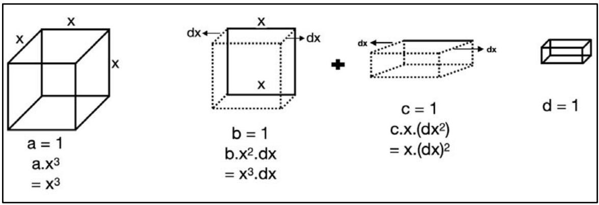Figure 15: Topological presentation of a polynomial $y = ax^3 + bx^2 + cx + d$ (a,b,c and are constants and $a = b = c = d = 1$ ) In figure 18, the $1^{\mathrm{st}}$ cube (from the left) shown has length of each side $= 1^{1/3} = 1$ (it has no differential term), the second term is a cube too with lengths of the 3 sides being x, dx and dx and only (1 cube since c = 1). The $3^{\mathrm{rd}}$ term is a cube of the lengths of the 3 sides being x, x and dx respectively and it is a single cube since b = 1. The fourth term is a homogeneous cube of length of each side being x and it is a single cube since a = 1. Now if the value of x changes infinitesimally small magnitude dx, then equation (58b) can be written as, considering the changed value of y is y1 and dy = (y1 - y). (topologically shown in Figure 18a above). $$ y _ {1} = \left(d ^ {1 / 3}\right) ^ {3} + c (x + d x) (d x) ^ {2} + b (x + d x) ^ {2} (d x) + a (x + d x) ^ {3} \tag {58c} $$ So, $\mathrm{dy} = (y_1 - y) = c\mathrm{dx} + 2b\mathrm{x}\mathrm{dx} + 3a\mathrm{x}^2\mathrm{dx}$ [the terms of $(\mathrm{dx})^2$ have been neglected](58d) Now the zeroth derivative of this new model would be, [considering the $1^{\mathrm{st}}$ term of equation (58d)] $$ \left(\mathrm {d y} / \mathrm {x} ^ {0}\right) = \mathrm {c d x} \tag {58e} $$ The first derivative, [considering the 2nd term of equation (58d)] $$ \left(\mathrm {d y} / \mathrm {x}\right) = 2 \mathrm {b d x} \tag {58f} $$ The 2nd derivative, [considering the 3rd term of equation (58d)], $$ \left(\mathrm {d y} / \mathrm {x} ^ {2}\right) = 3 \mathrm {a d x} \tag {58g} $$ Now the overall derivative of $y$ with respect to $x$ would be, $$ \left[ \frac{\mathrm{d y}}{\mathrm{x}} \right]_{\text{o v e r a l l}} = \left[ \left(\frac{\mathrm{d y}}{\mathrm{x}^0}\right) + \left(\frac{\mathrm{d y}}{\mathrm{x}}\right) + \left(\frac{\mathrm{d y}}{\mathrm{x}^2}\right) \right] / \left(\mathrm{x}^0 \mathrm{x}^1 \mathrm{x}^2\right)^{1/3} = \left[ (\mathrm{d y})_{\text{o v e r a l l}} / \mathrm{x} \right] = \mathrm{d x} [\mathrm{c} + 2\mathrm{b} + 3\mathrm{a}] = \mathrm{K d x} $$ $\left[\mathbf{x}\right.$ being the geometric mean of $\mathbf{x}^0$ $\mathbf{x}^1$ and $\mathbf{x}^2$, such that, $\mathbf{x} = (\mathbf{x}^{0}\mathbf{x}^{1}\mathbf{x}^{2})^{1 / 3}\big]$ Or, $\left[\mathrm{dy} / \mathrm{x}\right]_{\mathrm{overall}} = \mathrm{K.dx}$ $[\mathrm{K} = \mathrm{constant} = (\mathrm{c} + 2\mathrm{b} + 3\mathrm{a})]$ (58h) So, dy (at any point on the curve), as being obtained from equation (58d) is, $$ \mathrm {d y} = \mathrm {c d x} + 2 \mathrm {b x d x} + 3 \mathrm {a x} ^ {2} \mathrm {d x} $$ At the maxima or minimum for a certain value of $\mathbf{x}$, $\mathrm{dy} = 0$ and hence, $$ \left[ \mathrm {d x} \left(\mathrm {c} + 2 \mathrm {b x} + 3 \mathrm {a x} ^ {2}\right) \right] = 0 $$ Hence dx is not equal to zero, at the maximum or minimum, $$ \left(\mathrm {c} + 2 \mathrm {b x} + 3 \mathrm {a x} ^ {2}\right) = 0 \tag {58i} $$ So, either $\mathbf{x} = [-2\mathbf{b} + (4\mathbf{b}^2 - 12\mathbf{a}\mathbf{c})]$ (58j) Or, $\mathbf{x} = [-2\mathrm{b} - (4\mathrm{b}^2 -12\mathrm{ac})]$ (58k) Now for a concave upwards (convex downwards) curve, on any point of $\mathbf{x}$ (left side of the point of minimum), dy is negative towards the direction of increase of $\mathbf{x}$ and any point of $\mathbf{x}$ (right side of the point of minimum), dy is positive towards the direction of increase of $\mathbf{x}$. Now for a concave downwards (convex upwards) curve, on any point of $\mathbf{x}$ (left side of the point of maximum), dy is positive towards the direction of increase of $\mathbf{x}$ and any point of $\mathbf{x}$ (right side of the point of minimum), dy is negative towards the direction of increase of $\mathbf{x}$. Hence finding out the values of dy (of two points left and right) in the vicinity of the peak point, it can be easily found out whether the peak point is a peak maxima or peak minima. At the critical point, when the point of inflexion, point of minimum and point of maximum all do merge, the zeroth derivative, the $1^{\mathrm{st}}$ derivative, the second derivative,... [equations (58e), (58f), (58g)...] all become zero and the polynomial of equation (58a) does turn into, $$ y = d = \text {c o n s t a n t} \tag {581} $$ ## IV. CONCLUSION In conclusion, this article presents a critical reassessment of Newtonian Calculus, highlighting several foundational flaws and offering innovative corrections. It rightly identifies the issue with the Newtonian definition of the first derivative, or differential coefficient, which is based on a problematic limit process involving a vanishing denominator. The newly defined differential coefficient proposed here avoids this issue entirely. Furthermore, higher-order derivatives—such as the second, third, and fourth—are shown to suffer from circular definitions, rendering them conceptually unsound. For the first time in mathematics, differentiation has been demonstrated topologically using functions like $\mathbf{x}^n$, revealing that the true essence of differentiation lies in identifying the number of infinitesimal growth sites that emerge from a function. For instance, a linear function like $\mathbf{x}$ gives rise to a single differential element $\mathrm{dx}$, while a square function $\mathbf{x}^2$ yields two growth sites along the $\mathbf{x}$ - and $\mathbf{y}$ -axes, and a cube produces three—corresponding to $\mathbf{x}$, $\mathbf{y}$, and $\mathbf{z}$ directions. This leads to a new interpretation: the differential growth of a function $\mathbf{x}^n$ is simply $n \cdot \mathrm{d}\mathbf{x}$, making the conventional Newtonian derivative $\mathrm{d} / \mathrm{d}\mathbf{x}(\mathbf{x}^n) = n\mathbf{x}^{n-1}$ less a valid derivative and more a reflection of dimensional degradation. This dimensional interpretation is topologically validated for shapes like the square, circle, and sphere, giving physical meaning to formulas such as the derivatives of $\mathbf{x}^2$, $\mathbf{x}^3$, $\pi r^2$, and $4/3\pi r^3$, which had long been accepted without intuitive justification. Additionally, the article introduces a fresh perspective on integration, framing it not just as an inverse of differentiation but as a dimensional upgrade—an act of spatial hybridization through rotations and translations. The concept of the integration constant is revisited with clarity and rigor. It also critiques Newton's purely mathematical derivations of trigonometric function derivatives, which disregard the undefined behavior of trigonometric ratios at $0^{\circ}$ and $90^{\circ}$. In contrast, this work offers a topologically grounded, visually intuitive method of deriving these functions, making the subject far more accessible and engaging, especially for students. The article also demystifies the concept of $\pi \backslash \mathrm{pi}\pi$, explaining it through the idea of squeezing a circle—a concrete visualization that helps students grasp its true significance. Altogether, this work marks the beginning of a potentially transformative era in the study of mathematics. By offering an advanced, topology-based reformulation of calculus, it sets the stage for a richer, more intuitive understanding of the subject—one that could redefine how calculus is taught and comprehended going forward. Ethical Statement: Funding: This research did not receive any specific grant from funding agencies in the public, commercial, or not-for-profit sectors. Conflict of Interest: Ethical Approval: Ethical approval was not applicable for this study. Informed Consent: Informed consent was not required for this study. Data Availability Statement: Data sharing is not applicable to this article as no datasets were generated or analyzed during the study. 1. Stewart, J. Calculus: Early Transcendentals. Cengage Learning; latest ed. 2. Thompson, S.P., & Gardner, M. Calculus Made Easy. St. Martin's Press; revised ed. 3. Hass, J., Heil, C., & Weir, M.D. Thomas' Calculus: Early Transcendentals. Pearson; latest ed. 4. McMullen, C. Essential Calculus Skills Practice Workbook with Full Solutions. Zishka Publishing; 2010.

Generating HTML Viewer...