## I. INTRODUCTION Any building, bridge, dam, large construction object can be characterized by a set of natural oscillation modes. In seismology, these parameters are used to identify seismic stability of a construction. To understand what kind of vibrations could be endured by a construction during an earthquake (for the structure to remain), it is necessary to identify an accelerometer (i.e., identify accelerations during the earthquake in the construction location), conduct seismic microzoning (to understand how the upper part of the section would increase vibrations caused by an earthquake). Now, that we know these characteristics and oscillation modes of the object, we can solve the problem. There are two known methods for determining the amplitude-frequency characteristics of buildings and structures. The first, knowing in detail a construction design, to calculate theoretically these characteristics. The second is to determine experimentally. For the second one the "standing wave method" was developed and passed extensive practical tests on various objects [Emanov et al., 2002]. Using this method, we can determine the natural oscillation modes up to an extremely accurate level. For example, at the Sayano-Shushenskaya HPP (SSH HPP) dam, about a dozen oscillation modes were identified at different levels of reservoir filling. Determining these modes is not an easy task and it requires observations of seismic oscillations at hundreds (sometimes up to thousands) of points. In this case, we get the data in a time slice. The oscillation modes have such parameters at the moment of measurement, but what happens after a while? Builders are well aware [Hsu et al., 2020] that oscillation modes (and their frequencies) can change when an object is covered with cracks. The same way you can check integrity of crystal glasses in a store, by hitting the glass with a pencil and listening to it ring. If there is a crack in the glass, the frequency of the sound will decrease, due to loss of structural integrity of the material. Likewise, we would like to develop a monitoring system for buildings and constructions that tracks changes in natural frequencies over time. Here, we can also choose two ways: the first is to measure natural oscillation modes periodically and compare them with the calculated ones, locating places of the greatest discrepancies and studying them in more detail. The second is to begin monitoring changes in frequencies of different modes of natural oscillations. In particular, we note that in any case it is impossible to immediately observe changes in some frequencies, without proving that these are the frequencies of natural oscillations. Without sufficient experience, it is very easy to miscalcate some monochromatic oscillations for natural frequencies. Usually, while monitoring objects and surrounding areas, dozens of such oscillations are distinguished, some with high, and some with low quality factors. The first way is unfortunately quite expensive and can only be used for rather unique, very expensive objects. The second one is simpler and can be used by placing receivers not only inside a construction, but also at some reasonable distance from the location [Seleznev et al., 2012]. In this case, the object of study can be considered as a source of seismic vibrations. Imagine that this is a vibration source emitting not one, but a set of monochromatic oscillations equal to frequencies of natural oscillations. Based on the extensive experience of experimental and theoretical studies with powerful vibrators for more than 40 years [Alekseev et al., 1982], such an assumption can greatly simplify the task of knowing how seismic vibrations propagate from a vibrator, what they depend on, and how to accumulate these vibrations. First, the accumulation of monochromatic oscillations at adjacent points, it is possible to obtain significantly different oscillations in amplitude, since the waves from the source to the receiver at two different points follow different paths. Second, the directivity characteristic of a vibrator emitting monochromatic signals is highly dependent on near-surface conditions; and a vibrogram obtained far from the source at the same point can be radically different even when the ground is frozen to 10 cm [Solovyov et al., 2017]. Finally, if oscillations from the source are significant in amplitude and it is possible to admit a nonlinear interaction of the source with the ground, multiple, semi-multiple and one and a half multiple frequencies may be identified [Seleznev et al., 2019]. When emitting to inhomogeneous soils, the amplitude of multiple harmonics can exceed several times the amplitude of the main harmonic [Seleznev et al., 2019]. The Main Conclusion: It is not worthwhile to monitor changes in the amplitudes of natural frequencies coming from the object of study, since it is necessary to take into account many factors, including the fact that the object under study is still not a controlled vibrator, and depending on the wind load, operating mechanisms and other noises, the amplitude of the emitted signal can vary significantly. This leaves us with the possibility of studying changes in natural frequencies. But what could they change from? ## II. THEORY/CALCULATION Since any object can be described as a set of elements, including mass, damper and spring [Belostotsky et al., 2014a; Belostotsky et al., 2014b], the changes in natural frequencies emitted by the object will also depend on changes in the values of these parameters. Note, however, that significant change in frequencies, especially abrupt ones, could signal the destruction of the object. Below are several examples of engineering seismic monitoring of the large objects that show how natural frequencies can change with time. 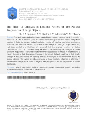Fig. 1 shows the SSH HPP dam, which has been studied by GS RAS specialists for more than a decade. It is a huge construction. The weight of the dam is approximately 20 million tons, the hydrostatic head on the dam is 18 million tons. In addition, the water level in the reservoir changes up to 40 meters every 6 months and, consequently, the added mass of the structure also varies. Researchers of the GS RAS have studied natural oscillation modes by the standing waves method for different fillings of the reservoir many times. Oscillations at hundreds of points in the body of the dam have been studied with three-component receivers. We now know which frequencies correspond to which modes of vibration (Fig. 2). 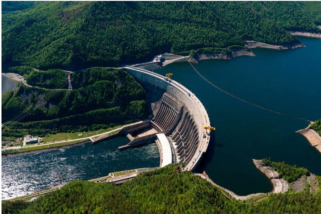 Fig. 1: The Sayano-Shushenskayadam (https://gelio/livejournal.com/)   Fig. 2: Spectral field of standing waves in the SSH HPP dam (a) and averaged spectra of resonance frequencies at the SSH HPP dam for 2018 (b) The seismological station, located at $4.5\mathrm{km}$ from the SSH HPP dam, has been carrying out digital registration of the seismic field for over 20 years. The possibility of identifying and tracking in time the frequencies of the first 7 modes of natural oscillations of the dam was investigated. It was determined that these frequencies are identified by the local maxima of amplitude spectrums of microseismic noise, recorded at the seismic station, averaged over 0.5-1.0 days [Liseikinet al., 2023]. If the length of the analyzed section of the seismogram is 200 seconds, the spectral resolution will be $0.005\mathrm{Hz}$. Even taking into account the background noise, it is possible to determine the values of the natural frequencies with an accuracy of not less than $0.01\mathrm{Hz}$. Fig. 3 shows the graph of change in the natural frequency of the 4th mode of dam oscillation at the SSH hydroelectric power station (as the most informative) and changes in the water level in the reservoir. It is clearly seen that in this case the main element (from the triad of mass, damper, spring) affecting the frequency values is the added mass of water. Smaller changes are also related to the mass of ice that freezes and breaks off the dam [Liseikin et al., 2023]. Why is it necessary to study the changes in natural frequency in detail? In the book "The Dam of the Sayano-Shushenskaya Hydroelectric Power Plant. State, Processes, Forecast" V. V. Tetelmin writes: "The safety problems of the SSH HPP dam are becoming more urgent and acute from year to year. Movements in the dam have not subsided, the base decompaction has been in progress, the contact seam has been opening, the arch stresses in concrete have been growing, the cracks in concrete of the pressure edge have not been stopped. Stress in the turbine water pipes and spiral chambers have also been growing. At the same time, specialists have not yet identified the reasons for such a deterioration in the dam" [Tetelmin, 2011]. Note that everything that V. V. Tetelmin writes about, affects the natural frequency values. To monitor and study such changes, it is necessary to increase measurements accuracy. This is quite possible, it is only necessary to increase the analysis interval on the seismogram, and put the recording station closer to the HPP in order to increase the signal-to-noise ratio. Note that it is not necessary to place the station at the HPP itself, since the method we use implies remote analysis, besides it is a dangerous construction with restricted access. 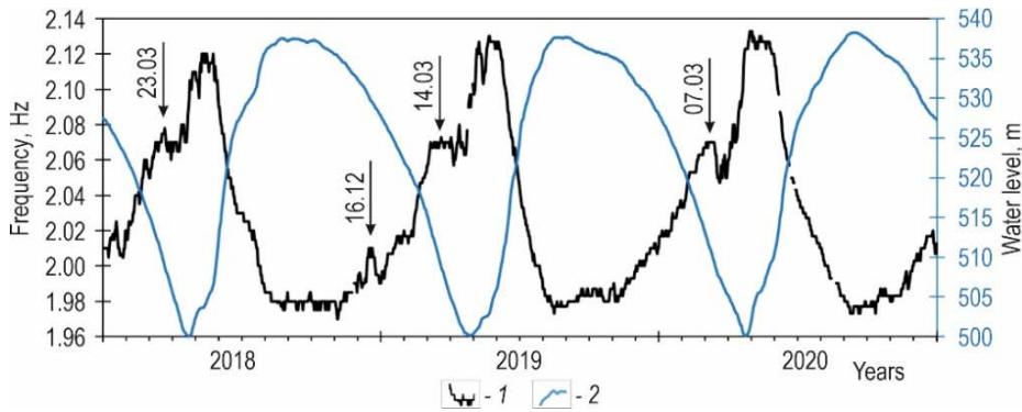 Fig. 3: Change in time of the fourth mode's frequency of natural oscillations of the Sayano-Shushenskaya HPP dam (1) with a change of the water level in the reservoir (2). Dates (23.03) highlight changes in natural frequency that are not related to changes in water level Another example of natural frequencies changing was obtained during an engineering seismic investigation of a residential 14-storey brick building in Novosibirsk. On the top floor of the building, a seismological station with a three-component $4.5\mathrm{Hz}$ seismic receiver had been continuously recording seismic data for two years. The directions of the seismic receiver axes are as follows: X - directed along the narrow part of the building, Y - along the long part of the building, Z - vertical. After analyzing the data for all the components, the X component was the most representative, which we will consider next. Fig. 4 shows the spectrogram for June 2022 and January 2023, and Fig. 5 shows the spectrum averaged over 12 hours (from 10:00 01/07/2023 to 10:00 01/08/2023).  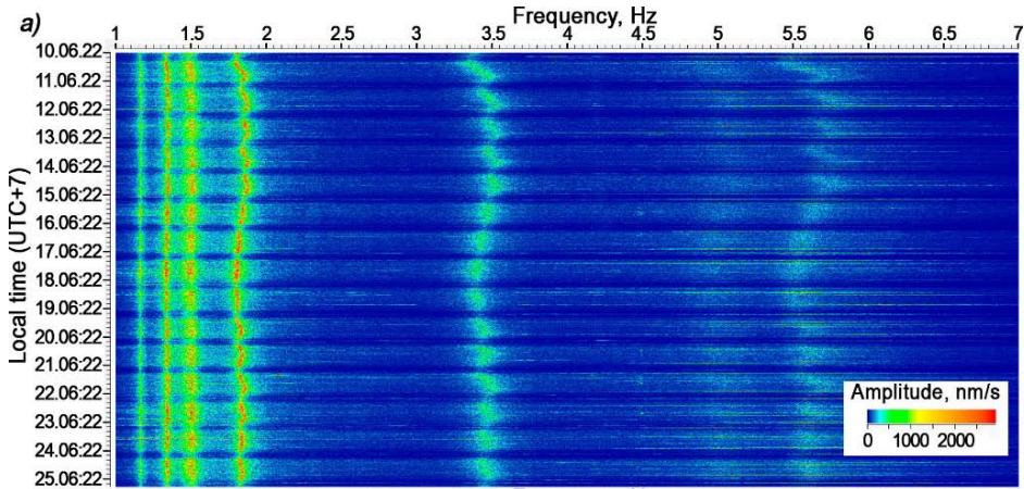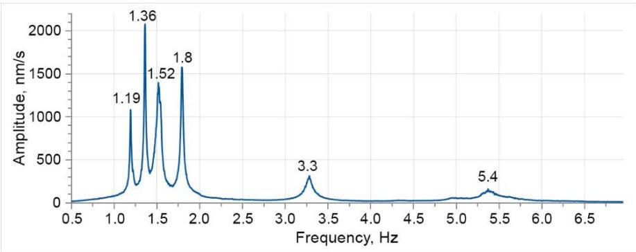  Fig. 4: Fragments of spectrograms for June 2022 (a) and January 2023 (b), X-components A special determination of oscillation modes by the standing waves method was not carried out here. However, evidence that the selected frequencies are the natural frequencies of the building can be provided by a simultaneous increase in vibration amplitudes at these frequencies during strong wind gusts (Fig. 4) or an earthquake of $M = 7.8$ that occurred in southern Turkey on February 6, 2023 (Fig. 6). The earthquake was very strong and it was possible to identify it using deconvolution, even when using a $4.5\mathrm{Hz}$ seismic receiver for registration. The earthquake appears only in the first frequencies. Therefore, we will only look at the spectrogram up to $3\mathrm{Hz}$. Fig. 6 shows that in the initial part of the earthquake recording, where there are waves with periods of about $1\mathrm{Hz}$, resonant excitation occurs at the natural frequencies of the building vibration and their amplitude increases by about 3 times. The study of the natural frequencies of the building showed that the frequency values change almost constantly over time, as can be clearly seen in Fig. 4. 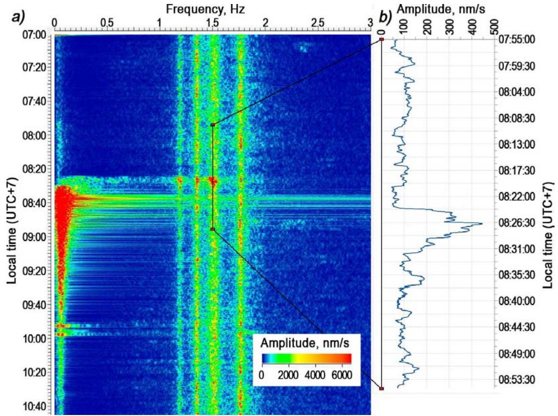 Fig. 6: Spectrogram of the Turkish earthquake on February 6, 2023, X-component (a). Graph of change in the oscillation amplitude at a frequency of $1.45\mathrm{Hz}$ in time (b) In the spectrograms in Fig. 4, obtained in the summer and winter months, the first 6 natural frequencies and their changes over time are clearly visible, as well as in the averaged spectrum in Fig. 5, where only the first four have the largest amplitudes. Some works [Cai et al., 2021] show that natural frequencies can be changed with temperature changes. In order to understand what these changes are connected with, we made graphs of changes in frequency of the fourth mode of natural oscillations (it has a high amplitude and sufficient fluctuations), variations in air temperature and the amount of precipitation, presented in Fig. 7 and Fig. 8. 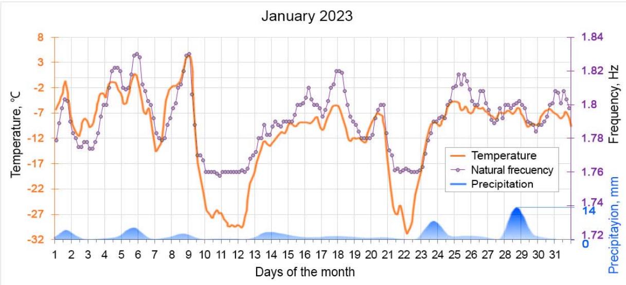 Fig. 5: Averaged spectrum for 12 hours from 01/07/2023 10:00 pm to 01/08/2023 10:00 am, X-component 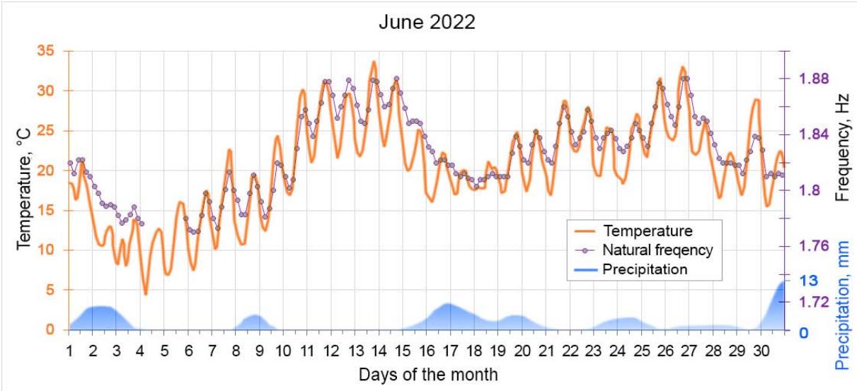 Fig. 7: Graphs of temperature changes, the frequency of the fourth mode of natural oscillations of the building and the level of precipitation in January 2023, X-component Fig. 8: Graphs of temperature changes, the frequency of the fourth mode of natural oscillations of the building and the level of precipitation in June 2022, X-component The processing of the received records was carried out using the software "SpectrumSeism", developed at the Seismological Brunch of GS RAS [Seleznev et al., 2021], which allows to convert seismic trace records into spectrograms. This makes it possible to determine how the amplitude-frequency composition of the record changes over time and to identify sources of oscillations of a particular frequency from the entire record. To obtain quantitative estimates, we generate graphs of changes in the amplitudes of oscillations at fixed frequencies by the short-time Fourier transform formula of the form: $$ A (\omega , t) = \frac {1}{T} \left| \int_ {t - T / 2} ^ {t + T / 2} f (\tau) e ^ {- i \omega \tau} d \tau \right| \tag {1} $$ where $f(\tau)$ -recorded seismic signal, $\omega$ -frequency for which the graph is generated, $t$ -running time, $T$ -time interval (window) in which the amplitude is identified,$|\ldots |$- modulus of a complex number. An important parameter in this method is the window length$(T)$, which directly determines the time resolution of the graph. However, it is not allowed to reduce the window length too much, because this reduces the frequency resolution. In summary, since natural frequencies are determined by seismic noise, in order to select a useful signal from them with a sufficiently high accuracy, the received seismic record is divided into fragments (windows), for each of which an amplitude spectrum is formed and averaged, resulting in an averaged spectrum without of noise, where only regular signals are detected. To select the values of natural frequencies, a large number of amplitude spectra of noise records were accumulated, as a result, sequences of local maxima corresponding to natural frequencies appeared on the averaged spectra. Fig. 7 and Fig. 8 show data on the X-component, i.e. transverse vibrations of the building, with the following parameters for formula Eq. 1: $T = 100s$, window step is 50s. This means that we cannot study signals with duration less than 100s. At the same time, the frequency resolution is $0.01\mathrm{Hz}$, so all signals on the seismogram with frequencies more than $0.01\mathrm{Hz}$ away from the frequency of the studied signal will not affect the result of amplitude determination according to formula Eq. 1. We chose the interval from 1.5 to $2\mathrm{Hz}$ (where one of the local maxima at a frequency of $1.8\mathrm{Hz}$, taken as the natural frequency of the building of the fourth mode, is clearly traced); and the graphs of its current values were generated over the averaged spectrum every 4 hours for January 2023 (Fig. 7) and June 2022 (Fig. 8). ## III. RESULTS Analyzing the variations of the curves shown in Fig. 7, we can note the following: precipitation practically does not effect changes in natural frequencies, even when about $40~\mathrm{cm}$ of snow fell on January 28-29 (with the roof area of about $600~\mathrm{m}^2$, the total snow weight is about 10 tons and the building weight is about 10 thousand tons with a perimeter of $100\mathrm{m}$, a wall thickness of $1\mathrm{m}$ and a height of about $40\mathrm{m}$ ). Besides the snow is periodically removed from the roof. The mass does not change significantly, but the damper and the spring change and it relates to the freezing of the brick wall. The structure of the building wall is shown schematically in Fig. 9. The inner part of the outer wall up to the 6th floor has a thickness of three bricks, from the 7th to the 14th floor - two. The insulation is foam with a thickness of $10~\mathrm{cm}$, then the outer facing part of the wall is one brick. The length of the brick is $25~\mathrm{cm}$.  Fig. 9: Scheme of a brick wall of the building In January 2023, there were severe frosts, and as the wall was freezing (Fig. 7), the natural frequency of the building also changed, but when the entire outer masonry was frozen to the foam, the changes in frequency stopped. Then the frequency began to change again until the moment when the temperature dropped to minus 20 degrees. Note that in winter the central heating in the building works, the colder it is outside, the more powerful the heating. This fact undoubtedly affects the natural frequencies in the form of local distortions, but does not have a significant impact on the overall picture because the indoor temperature remains almost the same. For a panel building, however, this influence is much more significant. During the summer period, the change in the frequency of natural oscillations is also closely related to the change in temperature (Fig. 8), and there is a noticeable slight lag in the frequency change from the temperature change. This can be explained by the thermal inertia of the building materials. 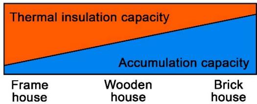 Fig. 10: Heat-insulating and storage capacity of different houses The thermal insulation capacity of a brick house is the lowest, so it is always recommended to insulate it, and the accumulation capacity is the highest (Fig. 10). It will take a lot of energy and time to heat a brick house, but it will also cool down more slowly than other ones [Kharitonov, 2017]. Therefore, Fig. 8 shows that in the June 1-4 and June 15-19 periods, natural frequencies decrease more smoothly than temperature and daily temperature changes are less noticeable in frequency changes. It should be noted that the temperature data were taken from the meteorological station of the Novosibirsk State University, located approximately 600 meters from the 14-storey residential building on Akademika Koptyuga Prospect 7 under study, and the precipitation data - from the weather station located 12 km from the object, which could make some error in the final result. ## IV. CONCLUSIONS The analysis of the obtained research results shows that natural frequencies of buildings and constructions are not static values and can vary within certain limits. It is determined that in the studied brick building, with an increase in ambient temperature, the frequency of natural oscillations increases, and with its decrease, the frequency value also decreases. The spectral-temporal analysis of long-term monitoring data at the Sayano-Shushenskaya HPP shows that it is possible to monitor changes in natural frequencies with an accuracy of not less than $0.01\mathrm{Hz}$ and a detail of the order of one measurement in half a day. Such accuracy and detail of measurements opens the way for solving many monitoring problems related to changes in the natural frequencies of the dam, which depend not only on a smooth change in the water level in the reservoir, but also associated with temperature changes, dam icing, changes in the sediment structure, erosion of the dam foundation and other reasons. It should be noted that such an accuracy and detail of measurements were obtained according to the data of the seismological station located $4.5\mathrm{km}$ from the dam. ## ACKNOWLEDGMENTS AND FUNDING The work was supported by Ministry of Science and Higher Education of the Russian Federation (075-00682-24). The data used in the work were obtained with large-scale research facilities «Seismic infrasound array for monitoring Arctic cryolitozone and continuous seismic monitoring of the Russian Federation, neighbouring territories and the world». The authors are grateful to colleagues from the Altai-Sayan and the Seismological Branches of GS RAS for valuable comments during the discussion of the article.

Generating HTML Viewer...

References

12 Cites in Article
A Alekseev,N Ryashentsev,I Chichinin (1982). How to look deep into the planet.
Alexander Belostotsky,Pavel Akimov (2014). Adaptive Finite Element Models Coupled with Structural Health Monitoring Systems for Unique Buildings.
A Belostotsky (2014). Experience of computational substantiation of the state of unique (high-rise and large-span) buildings and structures.
A Emanov,V Seleznev,A Bakh,A Krasnikov (2002). Standing Wave Method in Engineering Seismology.
A Liseikin,V Seleznev,A Emanov,D Krechetov (2023). Identification of natural oscillation frequencies of constructions from low-amplitude seismic signals (on the example of the Sayano-Shushenskaya HPP dam according to the monitoring data of 2001-2021).
V Seleznev,A Liseikin,I Kokovkin,V Soloviev (2012). Change of Natural Oscillation Frequencies of Buildings and Structures Depending on External Factors.
V Seleznev,A Liseykin,D Sevostyanov,A Bryksin (2021). SpectrumSeism. Certificate of registration of the computer program.
V Solovyov,V Kashun,S Elagin,N Serezhnikov,N Galeva,I Antonov (2017). Influence of seasonal changes of the environment under the vibrator CV-40 on the characteristics of its radiation (at vibroseismic monitoring of the Altai-Sayan region).
V Tetelmin (2011). Dam of the Sayano-Shushenskaya HPP: Status, processes, forecast.
A Kharitonov (2017). How tool use breaks down.
Ting-Yu Hsu,Arygianni Valentino,Aleksei Liseikin,Dmitry Krechetov,Chun-Chung Chen,Tzu-Kang Lin,Ren-Zuo Wang,Kuo-Chun Chang,Victor Seleznev (2020). Continuous structural health monitoring of the Sayano-Shushenskaya Dam using off-site seismic station data accounting for environmental effects.
V Seleznev,V Solovyev,A Emanov,V Kashun,S Elagin (2019). Features of radiation of powerful vibrators on inhomogeneous soils.
No ethics committee approval was required for this article type.
Data Availability
Not applicable for this article.
How to Cite This Article
V. S. Seleznev. 2026. \u201cThe Effect of Changes in External Factors on the Natural Frequencies of Large Objects\u201d. Global Journal of Research in Engineering - G: Industrial Engineering GJRE-G Volume 24 (GJRE Volume 24 Issue G1): .
Explore published articles in an immersive Augmented Reality environment. Our platform converts research papers into interactive 3D books, allowing readers to view and interact with content using AR and VR compatible devices.
Your published article is automatically converted into a realistic 3D book. Flip through pages and read research papers in a more engaging and interactive format.
This work is devoted to the development of the engineering seismic monitoring method created in GS RAS. In previous years, the “method of standing waves” was created and put into practice. It helps to separate natural oscillation modes of buildings and other engineering structures. The natural oscillations of hundreds of various objects (buildings, bridges, dams, etc.) had been studied and identified. We assumed that the physical condition of studied constructions could be controlled during exploitation by measuring the changes of natural oscillation frequencies. That would help to identify the appearance of defects in constructions, to prevent the risk of their destruction. However, it turned out that not everything is that simple: changes in frequency values are logically affected by changes in the environment around the studied objects. This article provides examples of these relations, influence of changes in environmental temperature, mass of objects and precipitation on the frequencies of natural oscillations.
Our website is actively being updated, and changes may occur frequently. Please clear your browser cache if needed. For feedback or error reporting, please email [email protected]
Thank you for connecting with us. We will respond to you shortly.