## I. INTRODUCTION Over the past several decades, the United States has experienced a tremendous increase in both job opportunities and workers' wage. However, this prosperity, since the middle 1980s, has not been proportionally shared by all the workers. Two trends, observed by many labor economists, help to explain this inequality: employment polarization and wage polarization. Employment polarization refers to the increasing concentration of employment in the highest and lowest-wage occupation groups, and the decreasing share of employment in the middle-wage occupation group. Wage polarization is the non-monotonic wage increase by the highest and lowest-wage occupation groups relative to the middle-wage occupation group. The foundation for a good interpretation and prediction is the "goodness of fit" or rather the robustness of the polarization phenomenon that is observed by many economists. The data on polarization has been always characterized by the U-shaped curve. It denotes the lag of the middle wage workers when compared to the top and the bottom segments. Mishel, Shierholz, and Schmitt, 2013 shows the change of the share of total employment between 1989 and 2000 in the U.S. by occupational mean log wage percentiles. The standard method of demonstrating job polarization is to give the simplistic view of how well the occupational employment data agreed with the underlying data. Lefter and Sand (2011) are one of the initial doubters regarding the robustness of the job polarization. They use the occupational employment growth trends from 1999-2002 March CPS data instead of 2000 Census data. The conclusion is the divergent pattern of occupational employment growth observed during the 1990s referred to as job polarization. It is largely the result of smoothing over extreme occupational employment changes that are mainly due to the revision of the occupational classification system prior to the 2000 Census. Mishel, Shierholz, and Schmitt (2013) also look at the data being used for the job polarization phenomena. For this purpose, they use the CPS-ORG data for occupational employment and wage trends. Because the CPS employment trends of the CPS data have not been used in the past for polarization studies, it could provide an additional verification of the sanguinity of the main data. Viewing the job polarization as absolute and relative also provides another perspective to look at the issue. Goos and Manning (2003) explored the disaggregation by occupation and industry. Goos, Manning, and Salomons (2010) also investigate the robustness of the regression used on the data. They look at the various countries of Europe for the effects of job polarization as a cross check. They conclude that the principal components are mechanically constructed. Additionally they have equal predictive power over recent occupational employment changes of the European countries. The previous robustness examination focused on different time periods or data quality; none of them have economics explanation in clarifying the robustness of the phenomenon. In the paper, I use data from similar points of a recession cycle in order to keep other influencing effects at bay which normally tends to make the data noisier, interferes with the statistical analysis, and can lead to erroneous or biased results. This means the two baselines of study will be on the peak or trough of the economic cycles. Additionally, decadal cycles and cycles found in other literatures would be studied. Another interesting question is the occupational structure of jobs in different skill levels. In other words, what kinds of jobs are driving the increase of the low-skill and the high-skill occupations? Autor and Dorn (2013) investigate the growth of low-skilled service occupations between 1980 and 2005. They find that the growth of service occupations accounts for most of the increase of the employment share and the workers' wage of the low-skill occupations. They use a counterfactual experiment to hold service occupations in 2005 at their 1980's level and find the increase of employment share is greatly damped as well as the wage increase. If the low-skill occupations are dominated by the service occupations, what is happening in the high-skill occupations? I examine the high-skill occupations and tries to figure out which occupation category accounts for the change of the employment share and the change of the wage. The paper fills the gap left by Autor and Dorm (2013) on the dynamics of wage and employment share polarization with emphasis on the top-end (high-skill) percentile. Is one group (s) of occupation pulling everyone in the top end up? Or maybe it is a monotonic increase of all high-skill occupations? My hypothesis is that the managers and professionals occupations play the most important role in accounting for the high-skill occupation growth. Similar to Autor and Dorm (2013), the counterfactual experiments are employed but applied to the high-skill workers and the time length is extended to 2013. Empirical evidence is provided to reveal that most of the change at the top end of the wage spectrum is accounted for by the change of the managers and professionals while other occupations play a relatively minor role. Besides the structural composition of the high-skill occupations, this paper also investigates a very important factor in determining the wage of high-skill occupations: the length of education. Acemoglu and Autor (2010) find that years of education contribute more to wage inequality in the recent years especially between college and non-college graduates. They use CPS data and plot the log hourly real wage in 1973, 1989, and 2009. Acemoglu and Autor (2010) offer a good presentation of impact of years of education on workers' wage. However, they do not account for the wage difference between different classes of works; high-skill, middle-skill, and low-skill. This paper separates the workers into three categories based on the skill level of the occupation and investigates how education impact wages for different skilled workers. More specifically, the length of education is measured at the level of education rather than years of education since the level of education is more credential oriented such as high school, college, or graduate degree rather than years in school. This paper is organized in the following ways. Section 2 discusses the data used in this paper. Section 3 explains the methods I use to examine the robustness of the polarization and details about the counterfactual experiment, as well as the model for the education effect on the wage. Section 4 discussed the results, the conclusions and potential explanations. The paper is concluded by section 6. ## II. DATA The article uses the Current Population Survey's Merged Outgoing Rotation Group (CPS MORG) data set. CPS is an individual-level monthly survey conducted by the government on household employment and labor information. It is the source of unemployment rate announced each month. The data is available from the Bureau of Labor and Statistics and National Bureau of Economic Research. The CPS administers 4 monthly household interviews, then ignores them for 8 months, then interviews them again for 4 more months. If an occupant of a dwelling unite move, they are not followed, rather the new occupants of the unit are interviewed. Since 1979, only households in month 4 and 8 have been asked their usually weekly earning. The information from the outgoing interviews forms the MORG, gathered by BLS at the end of each year. This paper uses date from January 1980 to December 2013 for the analysis and models. US Department of Labor's (DOT) classification of occupation changes several times during the sampling period. So, this paper utilizes the 330 occupations' classification (denoted as occ1990dd) designed by Dorn (2009) and composed by Gaggl and Eden (2014). Autor and Dorn (2013) matched the occupation code using the Census data, this paper uses the same occupations match but with CPS data. The CPS data is nosier than the Census, but it is more updated and detailed since CPS is conducted monthly. Despite the noise, CPS is a fair representation to check for robustness of the polarization phenomenon. ## III. METHODS AND MODELS The current population data (CPS) from the Bureau of Labor Statistics is used for this paper regarding unemployment rate correlated with other parameters like occupation from 1979 to 2013. All the data manipulation and statistical analysis has been achieved using the commercial software STATA. The data is first broken into yearly subgroups for further yearly calculations. Thereafter, calculate the employment share of each percentile for a specific year. This is done by first deflating the wage earned by the personal consumption expenditure (PCE). Then the mean log wage is calculated from this variable. The weighted mean of the mean log wage is thereby calculated. The percentile of mean wage is calculated for facilitating the final regression. Additionally, the employment share of the each percentile of the mean wage is evaluated. The data of employment rate versus percentile is a scattered variable. This procedure is used to calculate the change in employment rate versus wage percentile for all time points of interest. To calculate the rate in change of employment, the change in employment is subtracted across the different time points. A LOWESS smoothening algorithm is used with a bandwidth of 0.75 to develop a locally weighted regression. Different time domains are used to evaluate the robustness of the employment data. A point wise running regression is used to evaluate the 95 confidence interval. A two sample Kolmogorov-Smirnov test has been used to test the similarity of the polarization distribution. The labor market polarization distribution is examined with four time frames: The whole sample, decadal spans, business Cycle (annual), and business cycle (quarter). ## i. The Whole Sample The data year limits of the CPS data are 1980 and 2013. The rate in change of employment correlated with the wage percentile is shown in Figure 1.1. The change in real log hourly wage by wage percentile is in Figure 1.2. The lowess regression of the data along with the confidence interval is presented in Figure 1.3. To compare with the results in Autor and Dorn (2013), I also constructed the employment share and wage distribution for the sample from 1980 to 2005, as shown in Figure 2.1, 2.2, and 2.3. ## ii. Decadal Spans To investigate the robustness of job polarization across different decades, I split the sample into three subsamples: 1980-1990, 1990-2000 and 2000-2013. The results of the lowess regression for employment rate change, real log hourly wage by wage percentile for the decade 1980-1990 are shown in Figure 3.1 and Figure 3.2. The lowess regression with the confidence interval is in Figure 3.3. Similar curves have been created for the time spans 1990-2000 and 2000-2013 and are shown in Figure 4.1 to Figure 5.3. The samples are compared against each other using the Kolmogorov-Smirnov. The results of the tests are presented in Table 6.1. The visual representation of the three employment rate change graphs are shown in Figure 6. ## iii. Business Cycles (Annual) The labor mobility and economic conditions are different at different points in a business cycle, therefore, even though we may observe a polarization trend over the whole business cycle or over several business cycles, the evolvement of employment shares and wage may demonstrate different characteristics within a business cycle. To test the impact of business cycle on the observed polarization, I investigates the distribution of employment shares and wage over occupation skills when the underlying economy are in different phases of business cycles. The business cycle is a standard boom bust cycle. The data was obtained from the National Bureau of Economic Research in order to determine the economic peak and slump years. In this article, a peak to peak (1980-2001) and a trough to trough (1982-2009) comparison has been made. The peak to peak data was operated upon to determine the percentage change in employment rate and the hourly wage change versus the wage percentile. Figure 7.1 and 7.2 show the results. The lowess smoothening for the same period is shown in Figure 7.3. The mathematical operations on the trough to trough period produced the same graphs (Figure 8.1 to Figure 8.3). The two sample Kolmogorov-Smirnov test is performed to evaluate the statistical similarity between the time spans. The results are presented in Table 6.2. The employment rate change over the two periods are shown in Figure 9. ## iv. Business Cycles (Quarter) The business cycles are often characterized by steep changes in the parameters near the economic peak and trough. The use of the annual data tends to smoothen out some of these effects. Therefore, to time business cycles more accurately, I repeat the above analysis using quarterly definitions of business cycles. The peak to peak period is from June-August 1981 to February-April 2001. The trough to trough period is from February-April 1991 to May-July 2009. The two sample Kolmogorov-Smirnov test is performed to evaluate the statistical similarity between the time spans. The results are presented in Table 6.3. The visual representation of the two employment rate change graphs are shown in Figure 10. Dorn (2009) design an occupation classification dividing all the individual jobs into 330 consistent occupations, which establishes six broad categories based on the characteristics of jobs. The six broad categories are provided in Table 1. In thee counterfactual experiment, I gradually control the change of the managers and professional occupations by each sub-category and generate the counterfactual results to analyze the effect of this occupation group on the overall high-skill occupations. In the employment share counterfactual experiment, a set of occupations are selected as the controlled occupations, which means their change will be controlled in order to evaluate their effect on the change of the high-skill occupations. Meanwhile, two years (denoted as Year 1 and Year 2) are chosen for the experiment that the employment shares of the controlled occupations of Year 2 are controlled at the level of Year1. First, I calculate the occupational employment shares for all occupations in both Year1 and Year 2. Then for the controlled occupations, their employment share of Year 2 is set back to the level of Year1. In order to keep the total employment share of all occupations equal to 1, the employment share gap of the controlled occupations before and after adjustment is distributed to non-controlled occupations weighted by their original employment share. For example, suppose there are only 5 occupations in both Year 1 and Year 2: A, B, C, D, and E with the controlled occupations of A and B. Their occupational employment share is respectively 0.2, 0.2, 0.2, 0.1, 0.3 in 2013; 0.1, 0.1, 0.2, 0.3, 0.3 in 1980. After the counterfactual adjustment, the occupational employment share in 2013 is changed into 0.1, 0.1, 0.267, 0.133, 0.40. After this counterfactual adjustment, all the occupations are ranked by the mean log occupational wage and divided into 100 groups according to the percentile. Finally, the employment share change of each percentile between Year 1 and Year 2 is plotted and smoothed by a LOWESS regression. In the occupational wage counterfactual experiment, instead of changing the employment share of the controlled occupations, the mean log wage of the controlled occupations in Year1 is set back to their level at Year 2. Take the same controlled occupations for example. The mean log wage of Financial managers and Actuaries are 3.10 and 3.30 in 2013, 2.10 and 2.30 percent in 1980. After the counterfactual setting, their mean log wage in 2013 is 2.10 and 2.30 percent respectively. All the occupations are ranked by the adjusted mean log occupational wage and grouped by the percentiles after the counterfactual wage change. The mean log wage of each percentile is the average mean log wage of each occupation within the percentile weighted by the number of workers in each occupation. The change of mean log wage between Year 1 and Year 2 is generated in a similar way as described above. One potential problem in the counterfactual experiment is the unbalanced occupational categories across years. Some occupations appear in the data of recent years but not included in the data of previous years, vice versa. For example, the occupation 004 (Chief executive, public administrators, and legislators) is included in the data of 2013 but does not appear in the data of 1980. It does not mean in 1980 such occupations do not exist, just because in 1980 this kind of occupations was categorized in other occupation groups, like 022 (Managers and administrators, n.e.c.), instead of a specific group. Dorn (2009) designed this occupation code to make the census data balanced over time but it seems fail to balance the CPS data across years. To solve this problem, I use the following method. If the occupation appears in Year 2 but not in Year1, the employment share of this occupation in Year 2 is set to 0 in the counterfactual employment experiment; the wage of this occupation in Year 2 is the wage relative to the average wage of other controlled occupations which appear in both Year 1 and Year 2. In 1991 the CPS switch from year of schooling measure to a credential oriented measure. For example, prior to 1991, a high school student's year of schooling would be between 9 to 12 and college students would be 13 and beyond. After 1991, CPS focuses on an interviewee's highest level of school that has completed or highest degree received. Acemoglu and Autor (2010) focus on the former, and I focus on the later. I create five categories for level of education: not a high school graduate (NH), high school graduate (HS), some college but no degree or associate/vocational degree (SC), college graduate (CG), and graduate degree (GD). For each of the levels above, I match the pre-1991 data to post 1991's credential orientated data. The NH category, I match years of schooling from 0 to 11 years in the 1991 data set to 12th grade no diploma post 1991 data set. The HS category, I match year of schooling 12 years in the 1991 data set to high school graduate, diploma or GED in the post1991 data set. The most challenging matching the SC, CG, and GD. For SC, I match year of schooling 13 to 15 in the 1991 data set to 3 variable in the in the post1991 data set(some college but no degree, associate degree vocation, and associate degree academic program). I use the 13 to 15 because, on average, most students finish a college degree in four year. I match CG year of schooling 16 in the 1991 data set to bachelor's degree in the post 1991 data set for the same reason. The year of schooling measurement in the 1991 data set ends at 18. I match years of schooling 17 and 18 in the 1991 data set to the 3 variables (master's degrees, professional degrees, and PhDs) in the post 1991 data set. This matching process unifies the different measurements of the length of education across the CPS time periods. In this section, all the workers in the economy are divided into three categories; high skilled, middle-skilled, and low-skilled. Skills are based on occupation mean wage percentile ranking. The high-skilled are those whose occupations mean wage rank above the 80th percentile. The middle-skilled are those whose occupations mean wage rank between 30th and 80th percentile, and the low-skilled are below 30th percentile. The log of real hourly wage is used as the dependent variables. Age and the square of age are used to control for experiences, and its nonlinear effect. Five dummy variables are created based on the matching process to measure the education level of an individual. This concise model provides a simple way to detect the preliminary effect of education length on the high skill workers' wage. Even though other factors can also be controlled such as union jobs, private or public jobs, race, gender, and other qualities, a simple model gives us a general empirical results upon which I can decide the direction of next research step. Currently, this paper only use two years to compare the education effects. This paper tries to identify the impact of education level on high-skilled workers compared to the low and middle-skilled. More specifically, I examine how much does a college or graduate degree impact wage for these three classes of workers. I use the level of educations dummies represent the education level and generate the following models: $$ Ln(wage_{i\theta}) = \beta_0 + \beta_2 NH_i + \beta_3 HS_i + \beta_4 SC_i + \beta_5 GD_i + \beta_6 Age_i + \beta_7 Age_i^2 + \varepsilon_i $$ $$ Ln(wage_{i\theta}) = \beta_0 + \beta_2 NH_i + \beta_3 HS_i + \beta_4 CG_i + \beta_5 GD_i + \beta_6 Age_i + \beta_7 Age_i^2 + \varepsilon_i $$ Where: $\theta =$ Wage for high-, middle-, and low-skilled workers NH = Not a high school graduate $$ HS = High school graduate $$ $$ SC = Some college/associate or vocational degree $$ $$ CG = College Graduate $$ $$ GD = Graduate Degree $$ $\mathbf{i} =$ denotes individuals ## IV. RESULTS ### a) Robustness Examination of the Job Polarization Lefter and Sand (2011) are the initial doubters of the robustness of the phenomena of polarization. This article builds on their work and compares across the different time spans the robustness of the phenomena of job polarization. The various time spans provides a wide perspective and validation possibility of the phenomena. The curve shapes are similar in behavior. The hourly wage change has the U shape which indicates a bigger change at the extremities than at the middle. The confidence interval of lowess regression of the employment change has an hour glass shape. This is due to the fact that data on the extremities is less accurately predicted than the data near the center. The decadal data show a mixed change in the trends. While the 1980 and the 2000's data showed a more traditional U shape with a greater change in the extremities compared to the middle which is a strong indicator of job polarization. The 1990's decade is not compliant to that behavior. The two sample Kolmogorov-Smirnov test (Table 6.1) however has a p-value of 0.078 for the comparison between 1980-1990 and 1990-2000, indicating that the data streams were statically similar. Similar result is observed in the business cycle evaluation where the annual data spans are proved statistically similar by the KS test while the quarterly were not. All the data used here is the data for the US on a national scale. It would be also of interest to verify the polarization characteristics across states based on their industrial indices. The percentage change in the log hourly wage seems to be more consistent from the decadal and business cycles. The employment share variation however produces mixed results indicating similar correlations across certain spans and not across others. The employment share distribution overall indicates the presence of the polarization effect but in varied degrees and has different patterns across the sample period and different business cycles. No pattern was observed for the data streams that are found similar. This leads us to conclude that there is not consistency in the data of job polarization across various time spans. As a result, any conclusions of job polarization would not be by default valid across any time domains. Its validity would have to be verified by comparing the data from that time span with the current one. 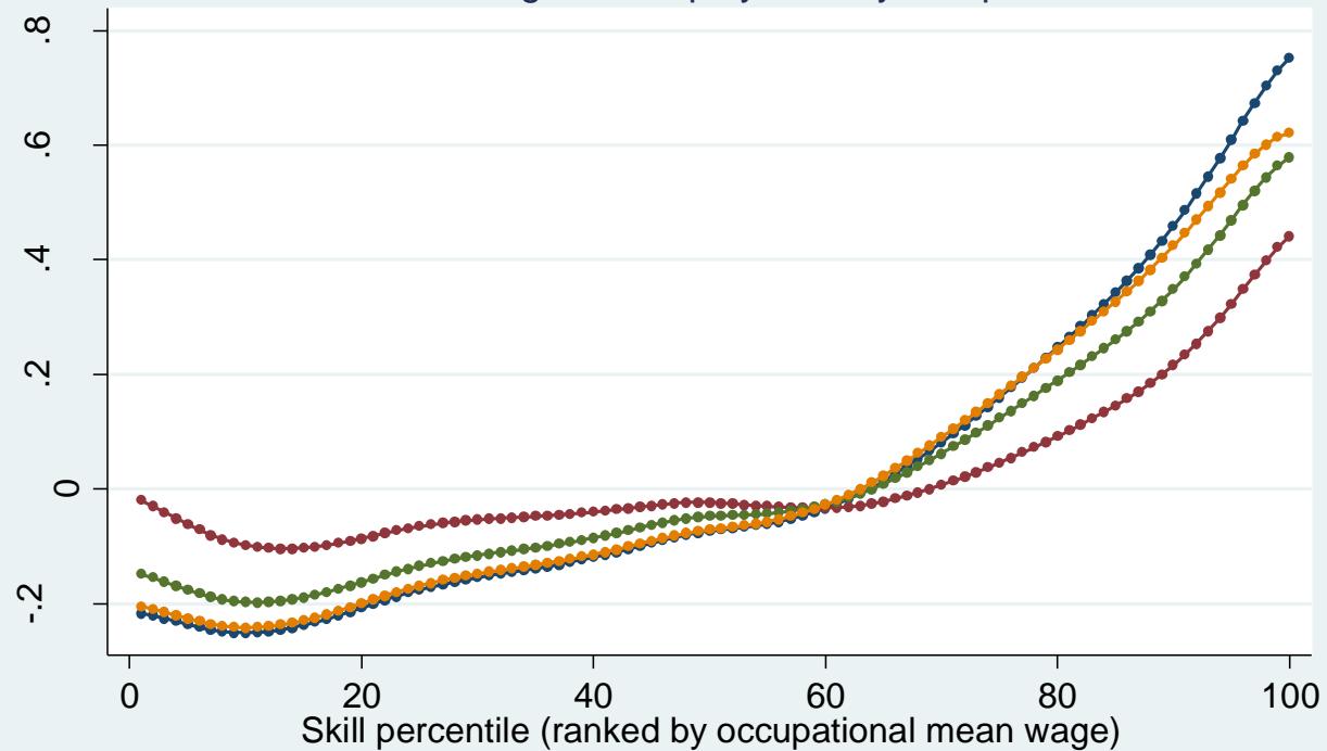The counterfactual experiment results are provided in Figure 11 and Figure 12. For both employment share and occupational wage, I choose Year 1 = 1980 and Year 2 = 2013. This period is consistent with the one in the robustness examination. In order to identify the driving occupation for the high-skill jobs, I gradually add the managers and professional occupations into the controlled group by each subgroup. According to the results, the managers and professional occupations play a very important role in the high-skill occupations. If employment share of this group is fixed at the 1980's level, a large proportion of the increase of the high-skill occupations is disappeared (Figure 11). Within this large group of occupations, A1 and A3 accounts for most of the employment share increase of the very top occupations, because controlling A1 and A1-A3 leads to a relatively large drop of the employment share change while controlling A1-A2 does not change the top employment share very much. Furthermore, considering absolute employment shares of these three groups (Figure 13), A1 group has the smallest absolute employment share but influences the highest paid occupation most. 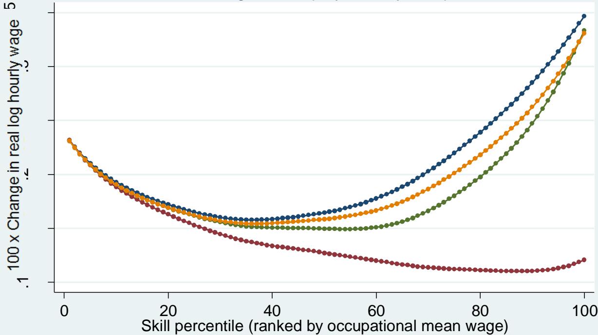For the counterfactual experiment in wage increase, the effect of the managers and professional group is much more obvious. If their wage did not change since 1980, all of the wage increase of high-skill occupations disappeared. Especially after controlling the A3 occupations, the wage increase is damped a lot compare with controlling the A1 and A 2. Actually, considering both Figure 11 and Figure 12, A2 occupations mainly cover the occupations from 80 percentile to 90 percentile, while the A1 and A3 occupations accounts for a very large portion of the occupations from 90 percentile to 100 percentile both in the employment share change and wage increase. ### c) Education Effect on the High-Skill Occupations Table 2- Table 5 summarizes the regression results. Table 2 and Table 3 use CG dummy as a base to look for the marginal effect of attaining a graduate degree comparing 1980 year to 2013. Table 4 and Table 5 use SC dummy as a base to look for the marginal effect of attaining a college degree comparing 1980 to 2013. ## i. Does Graduate Degrees Matter? In the 1980, the marginal benefit (hourly wage growth rate) for high-skilled workers attaining a graduate degree when they have a college degree is about $8\%$ hourly wage increase. For the middle-skilled and low-skilled workers it is about $11\%$ and $5\%$ respectively. However, in 2013, the result is different. The marginal benefit of attaining a graduate degree is $20\%$ for high skilled, $16\%$ for middle-skilled, and $3\%$ for low-skilled. The marginal benefit of getting a graduate degree is greater for middle-skilled than high-skilled workers in 1980. However, it is reverse in 2013. High-skilled workers enjoy more marginal benefit in 2013 than 1980 compare to the middle-skilled workers. The comparison of the low-skilled works between 1980 and 2013 is weak because the coefficient on GD is not statistically significant at the $10\%$ level. ## ii. Does College Degrees Matter? In the 1980, the marginal benefit (hourly wage growth rate) for high-skilled workers attaining a college degree when he has some college experiences or has an associate/ vocational degree is about $20\%$ hourly wage increase. For the middle- and low-skilled workers, it is $7\%$ and $3\%$ respectively in 1980. In 2013, high-, middle, low-skilled workers marginal benefits are $36\%$, $29\%$, and $21\%$ respectively. The high-skilled work gains the most marginal benefit in 1980 and 2013. However, the marginal benefit of college degree for middle-skilled workers grows fourfold from 1980 to 2013 and the marginal benefit of a college degree for low-skilled workers grows sevenfold from 1980 to 2013. This means the marginal benefit grew much more for middle- and low-skilled workers from 1980 to 2013. The regression results only control for experience by using age as a proxy variable. The result might be different if the model controls for more variables such as private or public jobs, the category of degrees (finance, math, art, history), or other variables. The goal is to determine the contributing factor of wage increase with respect to high-, middle-, and low-skilled workers. ## V. CONCLUSIONS The robustness of the polarization phenomenon is different for the employment share and wage increase based on my findings. The wage polarization seems to be more consistent for both the decadal and business cycles. The employment share variation however produced mixed results indicating similar correlations across certain spans and not across others. Even though, the employment share did overall indicate the presence of the polarization effect but various degrees and patterns are observed across time. No pattern was observed for the data streams that are found similar. This leads us to conclude that there is not consistent pattern in the data of job polarization across various time spans. According to the counterfactual experiment, the managers and professional occupations account for a large proportion of the employment share increase and almost all of the wage increase for the high-skill occupations. Specifically, the A1 and A3 group matters most for the top ten percentiles; the A2 groups covers most of the employment share and wage increase for the 80-90 percentiles. As for the education impact on the workers' wage, education becomes more and more important over time. More specially, the increase in marginal benefit of a graduate degree is mainly enjoyed by the high-skilled workers from 1980 to 2013. The increase in marginal benefit of a college degree is mainly enjoyed by the middle- and low-skilled workers. APPENDIX: TABLES AND FIGURES Table 1: Occupations Classification <table><tr><td>A. Managerial and Professional Specialty Occupations</td></tr><tr><td>A1. Executive, Administrative, and Managerial Occupations</td></tr><tr><td>A2. Management Related Occupations</td></tr><tr><td>A3. Professional Specialty Occupations</td></tr><tr><td>B. Technical. Sales, and Administrative Support Occupations</td></tr><tr><td>C. Service Occupations</td></tr><tr><td>D. Farming, Forestry, and Fishing Occupations</td></tr><tr><td>E. Construction Trades</td></tr></table> Table 6.1: Kolmogorov-Smirnov test for decadal spans <table><tr><td>Test Number</td><td>Group</td><td>D</td><td>p-value</td><td>Corrected</td></tr><tr><td rowspan="3">1</td><td>1980-1990</td><td>0.1300</td><td>0.185</td><td></td></tr><tr><td>1990-2000</td><td>-0.1800</td><td>0.039</td><td></td></tr><tr><td>Combined KS</td><td>0.1800</td><td>0.078</td><td>0.058</td></tr><tr><td rowspan="3">2</td><td>1990-2000</td><td>0.3800</td><td>0.000</td><td></td></tr><tr><td>2000-2013</td><td>-0.2700</td><td>0.001</td><td></td></tr><tr><td>Combined KS</td><td>0.3800</td><td>0.000</td><td>0.000</td></tr><tr><td rowspan="3">3</td><td>1980-1990</td><td>0.4000</td><td>0.000</td><td></td></tr><tr><td>2000-2013</td><td>-0.1500</td><td>0.105</td><td></td></tr><tr><td>Combined KS</td><td>0.4000</td><td>0.000</td><td>0.000</td></tr></table> Table 6.2: Kolmogorov-Smirnov test for business cycles-Annual <table><tr><td>Group</td><td>D</td><td>P value</td><td>Corrected</td></tr><tr><td>1980-2001</td><td>0.1800</td><td>0.039</td><td></td></tr><tr><td>1982-2009</td><td>-0.0700</td><td>0.613</td><td></td></tr><tr><td>Combined KS</td><td>0.1800</td><td>0.078</td><td>0.058</td></tr></table> Table 6.3: Two Kolmogorov-Smirnov test for business cycles-Quarter <table><tr><td>Group</td><td>D</td><td>P value</td><td>Corrected</td></tr><tr><td>1981Y7m--2001Y3m</td><td>0.2700</td><td>0.001</td><td></td></tr><tr><td>1991Y3m-2009Y6m</td><td>-0.3200</td><td>0.000</td><td></td></tr><tr><td>Combined KS</td><td>0.3200</td><td>0.000</td><td>0.000</td></tr></table>  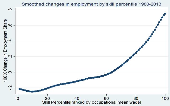Figure 1.1: Change in employment shares in U.S., smoothed and log difference, 1980-2013 (Whole Sample)   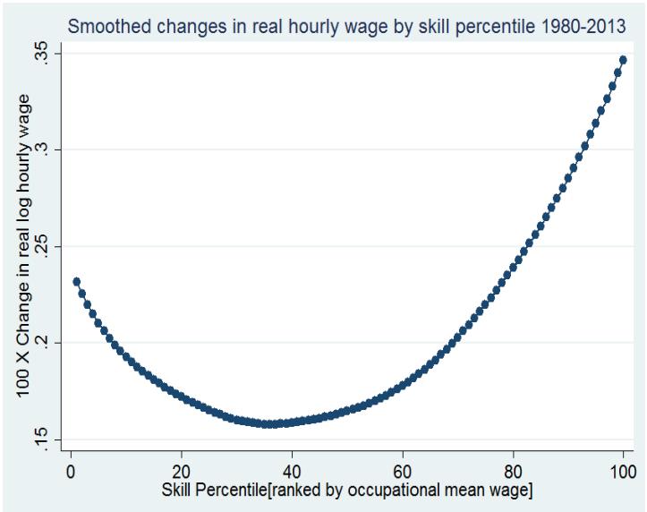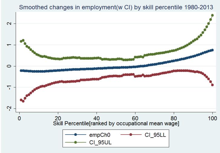Figure 1.2: Change in real log hourly wage U.S., smoothed and log difference, 1980-2013 (whole sample)  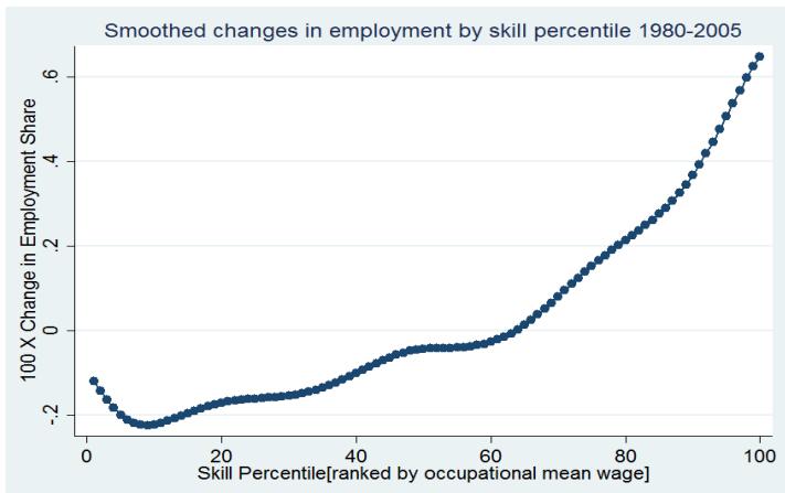Figure 1.3: Change in employment shares in U.S., smoothed and log difference with CI, 1980-2013 (Whole sample)  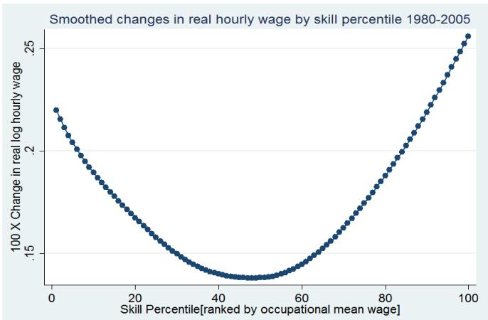Figure 2.1: Change in employment shares in U.S., smoothed and log difference, 1980-2005  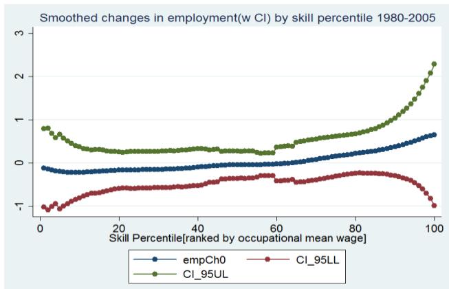Figure 2.2: Change in real log hourly wage U.S., smoothed and log difference, 1980-2005  Figure 2.3: Change in employment shares in U.S., smoothed and log difference with CI 1980-2005  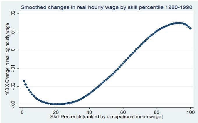Figure 3.1: Change in employment shares in U.S., smoothed and log difference, 1980-1990 (Decadal Span)  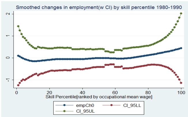Figure 3.2: Change in real log hourly wage U.S., smoothed and log difference, 1980-1990 (Decadal Span)  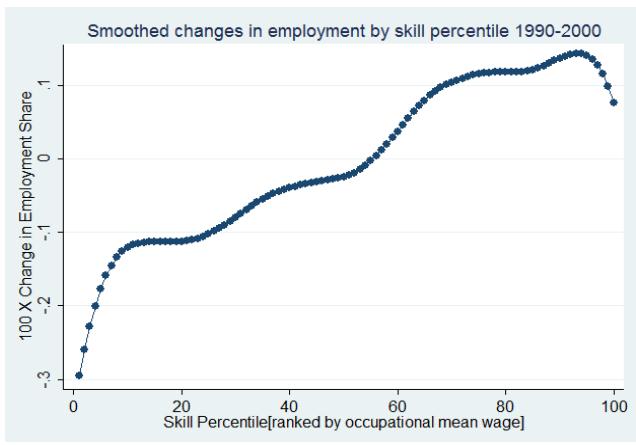Figure 4.1: Change in employment shares in U.S., smoothed and log difference, 1990-2000 (Decadal Span)  Figure 3.3: Change in employment shares in U.S., smoothed and log difference with CI: 1980-1990 (Decadal Span)  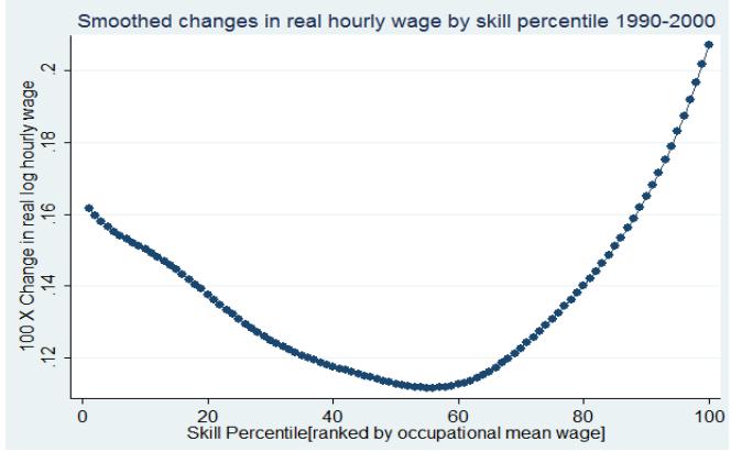Figure 4.2: Change in real log hourly wage U.S., smoothed and log difference, 1990-2000 (Decadal Span)   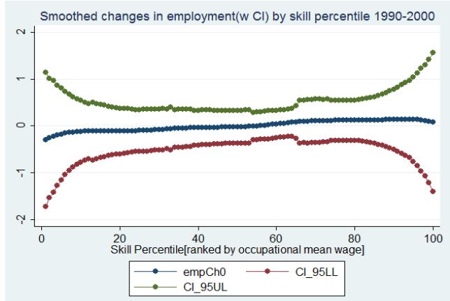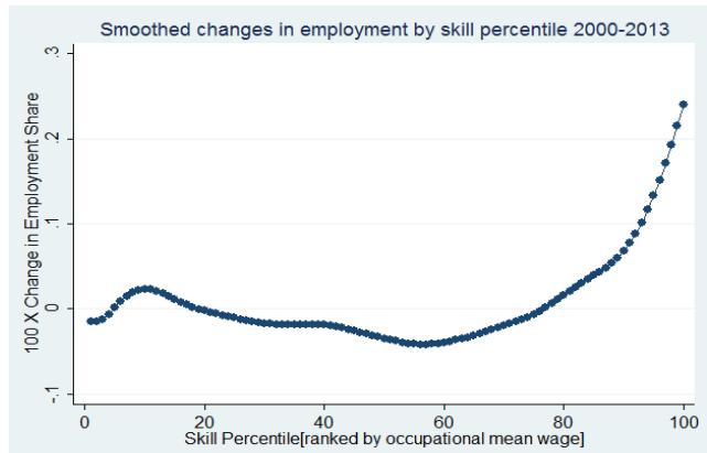Figure 4.3: Change in employment shares in U.S., smoothed and log difference with CI: 1990-2000 (Decadal Span)  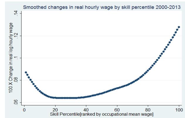Figure 5.3: Change in employment shares in U.S., smoothed and log difference, 2000-2103 (Decadal Span)  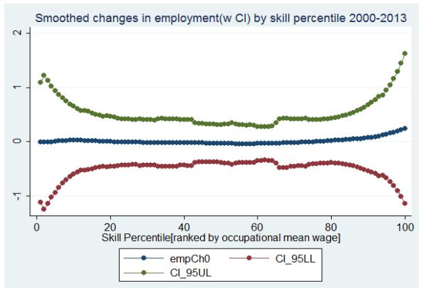Figure 5.1: Change in employment shares in U.S., smoothed and log difference with CI: 2000-2013 (Decadal Span)  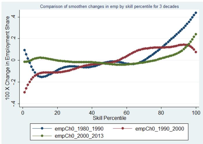Figure 6: Change in employment shares in U.S., smoothed and log difference for three decades  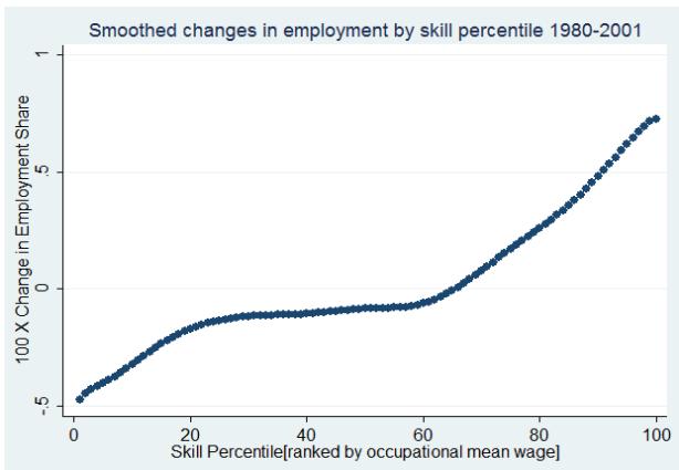Figure 7.1: Change in employment shares in U.S., smoothed and log difference, 1980-2001 (Business Cycle-Annual)  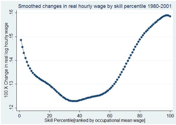Figure 5.2: Change in real log hourly wage U.S., smoothed and log difference, 2000-2013 (Decadal Span)  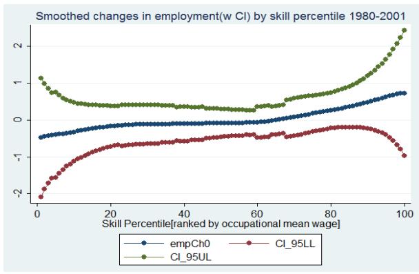Figure 7.2: Change in real log hourly wage U.S., smoothed and log difference, 1980-2001 (Business Cycle-Annual)  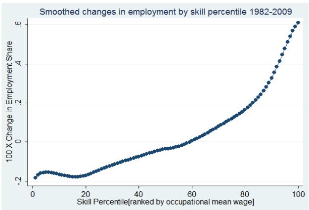Figure 8.1: Change in employment shares in U.S., smoothed and log difference, 1982-2009 (Business Cycle-Annual)  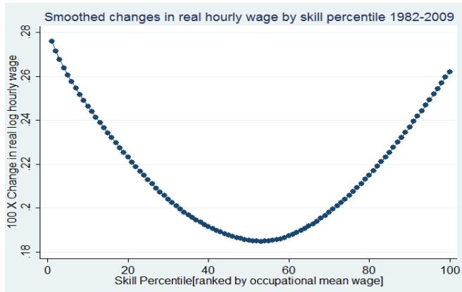Figure 7.3: Change in employment shares in U.S., smoothed and log difference with CI: 1980-2001 (Business Cycle Annual)  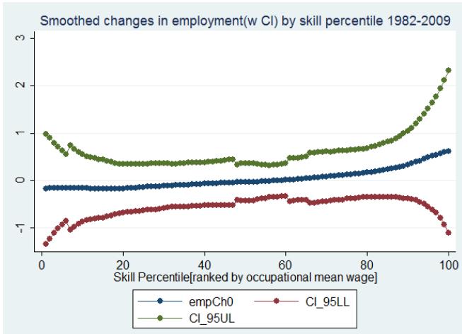Figure 8.2: Change in real log hourly wage U.S., smoothed and log difference, 1982-2009 (Business Cycl-Anmual])  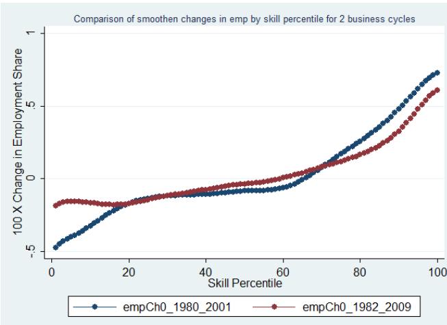Figure 8.3: Change in real log hourly wage U.S., smoothed and log difference, 1982-2009 (Business Cycle-Annual) Figure 9: Change in employment shares in U.S., smoothed and log difference for different business cycles  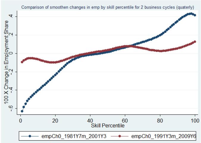Figure 10: Change in employment shares in U.S., smoothed and log difference (Business Cycle-Quarter)  Smoothed changes in employment by skill percentile  Figure 11: Counterfactual employment share change by skill percentile for 1980-2013 *A1 consists of 9 occupations, 2 is unbalanced. *A1 consists of 9 occupations, 2 is unbalanced. *A2 consists of 12 occupations, 5 is unbalanced. $^{*}$ A3 consists of 67 occupations, 7 are unbalanced.  Smoothed changes in employment by skill percentile - Lowess observed wage change control A1-A3 control A1-A2 control A1 *A1 consists of 9 occupations, 2 is unbalanced. *A2 consists of 12 occupations, 5 is unbalanced. *A3 consists of 67 occupations, 7 are unbalanced. 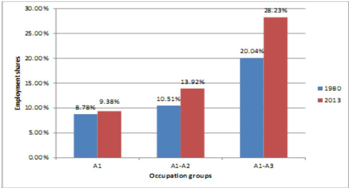 Figure 12: Counterfactual real log hourly wage change by skill percentile for 1980-2013 *A1 consists of 9 occupations, 2 is unbalanced. Figure 13: Employment shares of different occupation groups

Generating HTML Viewer...

References

16 Cites in Article
D Acemoglu (1999). Changes in unemployment and wage inequality: An alternative theory and some evidence.
D Acemoglu,D Autor (2011). Skills, Tasks and Technologies: Implications for Employment and Earnings.
David Autor,David Dorn (2013). The Growth of Low-Skill Service Jobs and the Polarization of the US Labor Market.
D Autor,F Levy,R Murnane (2003). The skill content of recent technological change: An empirical exploration.
D Autor,L Katz,A Krueger (1998). Computing Inequality: Have Computers Changed the Labor Market?.
W Baumol (1967). Macroeconomics of Unbalanced Growth: The Anatomy of Urban Crisis.
C Goldin,K Lawrence (2008). The Race between Education and Technology.
(2024). The Robustness of Job Polarization and the Growth of High-Skill Occupations Global Journal of Management and Business Research ( B ) XXIV Issue II Version I Year.
Maarten Goos,Alan Manning (2007). Lousy and Lovely Jobs: The Rising Polarization of Work in Britain.
Maarten Goos,Alan Manning,Anna Salomons (2009). Job Polarization in Europe.
M Goos,A Manning,A Salomons (2010). Explaning job polarization in Europe: the role of technology.
A Lefter,B Sand (2011). Job Polarization in the US: A Reassessment of the Evidence from the 1980s and 1990s.
Lawrence Mishel,Shierholzh,J Schmitt (2013). CHAPTER 6 Policy Decisions’ Role in Wage Suppression and Inequality.
J Van Reenen (2011). Wage inequality, technology and trade: 21st century evidence.
Maya Eden,Paul Gaggl (2014). The Substitution of ICT Capital for Routine Labor: Transitional Dynamics and Long-Run Implications.
D Dorn (2009). Essays on inequality, spatial interaction, and the demand for skills.
No ethics committee approval was required for this article type.
Data Availability
Not applicable for this article.
How to Cite This Article
Zekun Wu. 2026. \u201cThe Robustness of Job Polarization and the Growth of High-Skill Occupations\u201d. Global Journal of Management and Business Research - B: Economic & Commerce GJMBR-B Volume 24 (GJMBR Volume 24 Issue B2): .
Explore published articles in an immersive Augmented Reality environment. Our platform converts research papers into interactive 3D books, allowing readers to view and interact with content using AR and VR compatible devices.
Your published article is automatically converted into a realistic 3D book. Flip through pages and read research papers in a more engaging and interactive format.
The job polarization in the U.S. labor market has been widely discussed. This paper uses the CPS-MORG data to examine the robustness of the polarization phenomena to different time periods and business cycles. A special focus is on the high-skill occupations. This paper investigates the structural characteristics of the high-skill occupations and also reveals the education effect on the wage increase of the high-skill jobs relative to low-and middle-skill occupations. Based on the results, the wage polarization is robust to both time periods and business cycles while the employment share polarization is very sensitive to both. According to the counterfactual experiment, the managers and professional occupations account for a large proportion of the employment share increase and almost all of the wage increase for the high skill occupations. The increase in marginal benefit of a graduate degree is mainly enjoyed by the high-skilled workers from 1980 to 2013. The increase in marginal benefit of a college degree is mainly enjoyed by the middle-and low-skilled workers during the same period.
Our website is actively being updated, and changes may occur frequently. Please clear your browser cache if needed. For feedback or error reporting, please email [email protected]
Thank you for connecting with us. We will respond to you shortly.