This article describes the methodology for assessing the energy efficiency of pumping systems equipped with a variable electric drive and operating with variable load, which was elaborated by the authors of the article. The analysis of traditional methods of recalculating the characteristics of the efficiency of pumping units when changing the frequency of rotation of the impeller using the formulas of theories of hydrodynamic similarity of blade blowers is presented. It is shown that in the derivation of the similarity formulas assumptions were made, which were not fully confirmed later when testing operating pumps. An algorithm and a technique developed by the authors are presented that allow one to read the actual values of the efficiency from the pre-digitized universal characteristics of vane blowers The results of comparison of efficiency values calculated by different methods are presented.
## I. INTRODUCTION
A considerable part of the energy-efficient technological processes used in the national economy are quasi-stationary. They include, for instance: cold and hot water supply, water disposal, heat supply, etc. Since these processes are, as a rule, of accidental and random nature, the governing parameters (flow, head, and pressure) are subject to significant changes in the course of time. This presents great challenges for the proper selection of vane blowers (such as rotodynamic vane pumps, fans, smoke exhausters, and air blowing machinery) as well as complicates their control noticeably.
The existing regulatory and technical literature [1-7] recommends that the selection of parameters for rotodynamic vane blowers operating with variable load should be done using extreme parameters arising at peak loads. This approach is based on the reliability principle as the characteristics of the installed equipment covering the peak load can ensure coverage of any other current load with a considerable reserve. Processing of the statistical data which characterize the operation of equipment with reliable load in engineering systems shows that the probability of arising of a peak load within a year is insignificant while its time duration amounts to approximately $2 - 3\%$. That is why the equipment operates most (major part) of the time under the modes which differ substantially from the extreme ones.
The processing of the statistical data, which characterize the operation of equipment with reliable load in engineering systems, shows that the probability of arising of a peak load within a year is rather insignificant while its time duration amounts to approximately $2 - 3\%$. That is why, the equipment operates most (major part) of the time under the modes which differ substantially from the extreme ones.
In compliance with the traditional methodology for selecting parameters of rotodynamic vane blowers, their flow under the optimal mode of operation $Q_{\mathrm{opt}}$ is assumed to be equal to the maximal load value $Q_{\mathrm{max}}$; that is the following condition shall be fulfilled: $Q_{\mathrm{max}} = Q_{\mathrm{opt}}$. The maximal value of efficiency corresponds to the optimal flow $Q_{\mathrm{opt}}$, so with the traditional technique for selecting such rotodynamic vane blowers, the following condition shall be satisfied: the maximal value of efficiency shall correspond to the optimal flow. Since all the current flow values in this case are found to be lower than the maximal (peak) load, their coverage corresponds to the rotodynamic vane blowers' operation in the underload modes. Herewith, there is a displacement of the vane blower's operation modes into the region of low values of efficiency, which leads to an excessive energy consumption and, consequently, to a low energy efficiency of operation of the blowing system on the whole.
Testing and mathematical simulation for the existing pumping systems indicate that efficient operation of the rotodynamic vane blowers under variable load can be achieved if two conditions are met simultaneously: firstly, high efficiency values of the pump itself and, secondly, maximal binding of its characteristics to the parameters of the system where it will be installed. Researches show that the efficient operation of the blowing system under variable load will be composed from a set of efficiencies of its operation in separate modes that compound the process. The basic parameters that form the actual operation modes are as follows: the flow rate is $Q$, head — $H$, and efficiency — $\eta$. If the water consumption value is set by the system, then the head $H_j$ and efficiency $\eta_j$ (at the flow $Q_j$ ) depend in great measure on the validated method of control of the pumping unit, as well as on the parameters of the technology process supported by the rotodynamic vane blower.
Analysis of the energy efficiency of the blower operation under the current operation modes requires determination of the head (pressure), efficiency, useful and consumed power in each of the statistical intervals described by the process histogram. To obtain the needed accuracy of estimating the head and efficiency values that form the values of the consumed power in any considered statistical interval, it is necessary to determine their number correctly to ensure adequacy of describing the real physics processes by a mathematical model that replaces them. In order to achieve the accuracy of estimating the head and efficiency demanded for practical calculations, it is essential, as the studies have shown, that the gradients of these parameters $(\Delta H / \Delta Q$ and $\Delta \eta /\Delta Q)$ in the limits of each considered statistical interval be not greater than $1.5 - 2\%$.
The on-site investigations of the water supply and heat supply systems carried out by the SPL "Energosit" show that the efficiency of the rotodynamic vane blowers operating with variable load is affected greatly by a wide range of factors, namely: the range of consumptions used by the system and distribution of their probabilities within this range, the position of the optimal flow $Q_{\mathrm{opt}}$ and efficiency of the rotodynamic vane supercharge towards the placement of the load (flow) range, as well as the $Q_{\mathrm{opt}}$ position relative to the flow at the blower's operating point. Besides, when the proportional method of control is used and at minimizing the exceeded heads, the energy efficiency of the rotodynamic vane pump operation is affected significantly by the hydraulic exponent of the system (i.e. the relation $a = H_{st} / H_{req}$, where $H_{st}$ and $H_{req}$ are the static and required heads of the system).
Do the accepted traditional methods of selecting rotodynamic vane blowers take into account the impact made by the above factors on the selection?
For sure, they do not, as binding of the pump characteristics to the system parameters is done using one single point with the coordinates $Q_{\mathrm{opt}}$ and $H_{\mathrm{opt}}$, which is true only when a rotodynamic vane blower with a steady load or close to this is operating. Extrapolation of the traditional technique for selection of rotodynamic vane superchargers equipped with VFD and operating with variable load does not permit us to make a maximal binding of the rotodynamic vane blower characteristics to the system parameters, without sufficient substantiation and correction (or without replacement of this technique to a new one). In the absence of such binding, one of the two conditions described above and being required will ensure the best efficiency of pumping systems.
The Scientific and Practical Laboratory "Energosit" has been performing the researches on the enhancement of energy efficiency of rotodynamic vane blowers operating with variable load in water supply, water disposal and heat supply systems for more than ten years. The research is being done in frames of the energy service contracts when payment for the fulfilled work is made from the resources obtained through power saving that is achieved as a result of modernization of the operating pumping systems by way of selecting the optimal characteristics of the installed rotodynamic vane blowers relative to the parameters of the operating systems as well as by way of selecting the most efficient techniques of their control. The work under the energy service contracts requires a thorough instrumental examination of the validating operating systems having the purpose of obtaining objective and reliable data on the evaluation of the existing power saving potential.
Since mistakes in defining the power saving potential may lead to economically unsubstantiated decisions and unjustified investment, the authors of this study have worked out and tested in practice the technique for evaluation of the energy efficiency of operation of pumping systems. As for most of the technology processes supported by rotodynamic vane blowers the change in the load (flow) takes place rather slowly, the duration of the process can be split into separate static time intervals, in the limits within which it is allowed to consider, with a reasonable degree of accuracy, the flow, head and efficiency as being constant. This permits one to determine the energy consumption of the pumping unit through numerical integration for any considered time period, for instance, one year:
$$
S_{\mathrm{w}} = \sum_{\mathrm{j}=1}^{\mathrm{m}} \frac{\rho\mathrm{g}Q_{\mathrm{j}}H_{\mathrm{j}}}{1000\eta_{\mathrm{jpu}}\eta_{\mathrm{jmot}}\eta_{\mathrm{jdr}}} p_{\mathrm{j}} T \tag{1}
$$
$\rho$ is the density of the liquid, $kg/m^3$; $g$ is the free-fall acceleration, $m/s^2$;
$Q_{j}, H_{j}$ are the flow and head of the rotodynamic vaneblower in the $j$ -th interval of flows, $m^{3} / s$, m.w.c;
$\eta_{jpu m}, \eta_{j m o t}, \eta_{j d r}$ are the efficiencies of the rotodynamic vane blower, electric motor and electric drive in the $j$ -th statistical interval;
$p_{j}$ is the probability of the flow $Q_{j}$ in one year;
$T$ is the time of the pump operation during one year (hour);
mis the number of members in a statistical series.
For the pumps equipped with a variable-frequency drive (VFD), the head characteristic and efficiency characteristic may be represented in the form:
$$
H_{\mathrm{j}} = A_{\mathrm{n}} Q_{\mathrm{j}}^{2} + K_{\mathrm{T}} B_{\mathrm{n}} Q_{\mathrm{j}} + K_{\mathrm{T}}^{2} C_{\mathrm{n}} \tag{2},
$$
$$
\eta = D_{n} Q_{\mathrm{j}}^{2} + E_{n} Q_{j} + F_{n}
$$
where
$A_{n}, B_{n}, C_{n}, D_{n}, E_{n}$ and $F_{n}$ are the approximation coefficients of the pump characteristics;
$K_{T} = \frac{n_{C}}{n_{N}}$ is the coefficient of the rotation frequency change;
$n_{C}$ and $n_{N}$ are the current and nominal rotation frequencies of the impeller of the rotodynamic vane pump.
In the case when a VFD is used, recalculation of the characteristics of rotodynamic vane blowers in terms of the current frequency of the impeller rotation, which is different from the nominal one, is done using the formulas received from the theory of hydrodynamic similarity of rotodynamic vane blowers. The formulas for the recalculation of the flow, head and power have the following form in such a case:
$$
\frac{\mathrm{Q} _ {\mathrm{C}}}{\mathrm{Q} _ {\mathrm{N}}} = \mathrm{K} _ {\mathrm{T}} \tag{4}
$$
$$
\frac{\mathrm{H} _ {\mathrm{C}}}{\mathrm{H} _ {\mathrm{N}}} = \mathrm{K} _ {\mathrm{T}} ^ {2} \tag{5}
$$
$$
\frac{\mathrm{Nc}}{\mathrm{N}_{\mathrm{N}}} = \mathrm{K}_{\mathrm{T}}^{3} \tag{6}
$$
where
$Q_{\mathrm{C}}, H_{\mathrm{C}}, N_{\mathrm{C}}$ are the current values of the flow, head and supplied power for the current frequency of the impeller rotation $n_{c}$:
$Q_{N}, H_{N}, N_{N}$ are the same for the nominal frequency of the impeller rotation $n_{C}$.
The use of formulas (4) and (5) permits one to determine with a high degree of accuracy the values of flow and head when the frequency of the impeller rotation is changed, which allows one to obtain a new position for the head characteristic of the pump in the H-Q coordinates (Fig.1).
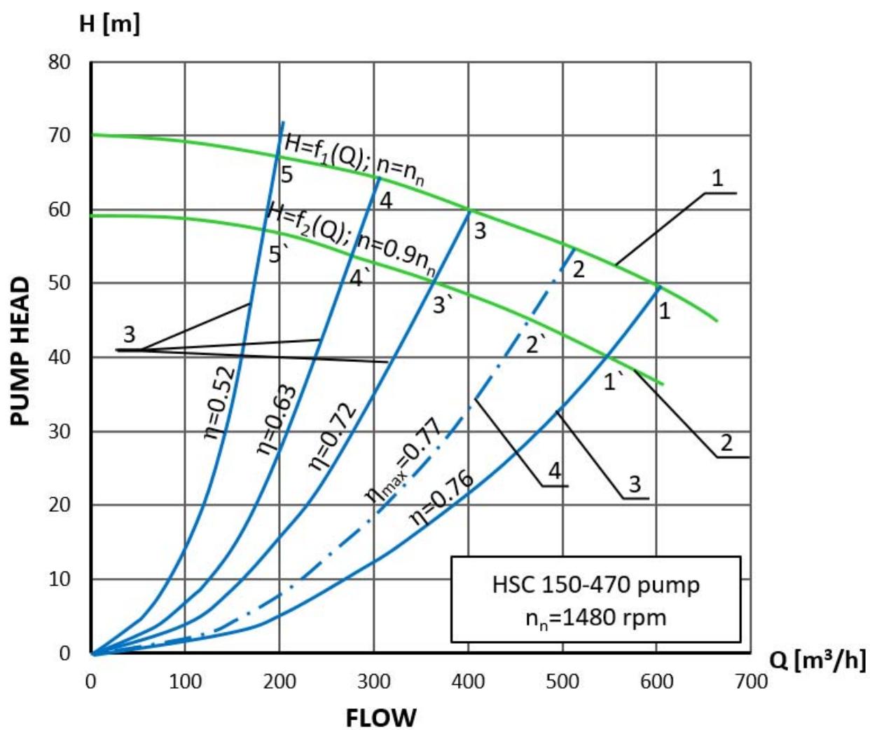
Figures for this Study (including captions) Fig. 1: For the Recalculation of the Characteristics of a Rotodynamic Pump using the Formulas of Hydrodynamical Similarity
1. The head characteristics of the pump for the nominal rotation frequency of the impeller $(\mathrm{n_n} = 1480~\mathrm{rpm})$
2. The head characteristics of the pump at the reduction of the rotation frequency $(n = 0,9n_{\mathrm{n}} = 1330~\mathrm{rpm})$
3. The curves of similar modes (CSM);
4. A curve of similar modes of the maximal value of efficiency.
Fig. 1 displays the head characteristic $\mathsf{H}_1 = \mathsf{f}_1(\mathsf{Q})$ for the nominal $(n_{\mathrm{N}} = 1480~\mathrm{rpm})$ and decreased (current) frequency of rotation $(n_{\mathrm{C}} = 0.9$, $n_{\mathrm{N}} = 1330$ rpm) of the impeller $\mathsf{H}_2 = \mathsf{f}_2(\mathsf{Q})$. The initial position of the head characteristic for the nominal frequency of the impeller rotation H-Q (see Fig. 1, pos. 1) and its position at decreased rotation frequency are given in the figure (see Fig. 1, pos. 2). Fig. 1 also presents the curves of similar modes (CSM), i.e., the equal level curves of efficiency (see pos.3). In compliance with the theory of hydrodynamic similarity, as the rotation frequency reduces, point 5 (see Fig. 1) shifts to position $5'$ (4 to $4'$ ), etc. Displacement of each point of head characteristics 1, 2, 3, 4, 5 to positions $1', 2', 3', 4'$ and $5'$ (see Fig.1) occurs by the parabola $\mathsf{H}_{\mathrm{j}} = \mathsf{K}_{\mathrm{j}}\mathsf{Q}^2$, that is by the curve of similar modes (CSM). When formula (6) is used for recalculation of the consumed power, it is supposed that the efficiency values along the parabola of similar modes do not change, i.e. $\eta_5 / \eta_{5'} = 1$, $\eta_4 / \eta_{4'} = 1$, etc.
It is known that the actual efficiency values at the change of the impeller rotation frequency in the rotodynamic vane blower can be received only by way of performing bench tests at different frequencies of its rotation.
This allows to obtain the so-called universal (control) characteristics of the rotodynamic vane blower. As an example, the control characteristic of the WiloCronoNormNL-125/200 ( $n_N = 2900$ rpm) vane blower is given in Fig. 2.
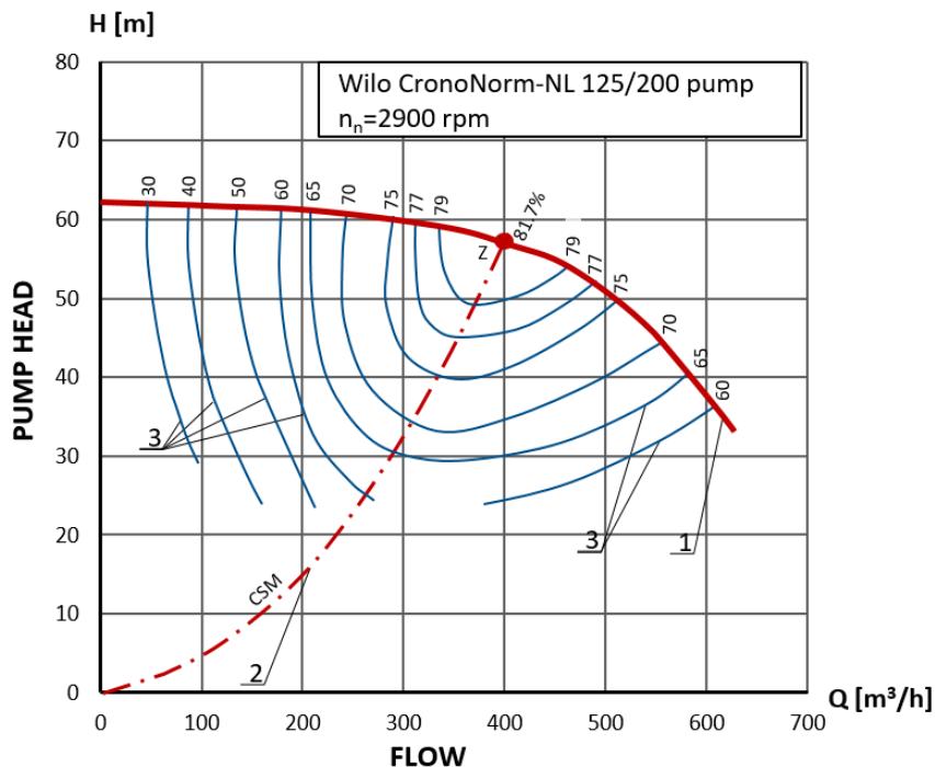 Fig. 2: The Universal (Control) Characteristics of the Pump
1. The head characteristics of the pump $(\mathsf{n}_{\mathrm{c}} = \mathsf{n}_{\mathrm{p}})$
2. A curve of similar modes of the maximal value of efficiency;
3. The efficiency equal level curves.
Fig. 2 displays the head characteristic of the pump (see pos.1) for the nominal rotation frequency of the impeller, the curve of similar modes (CSM) of the maximal value of efficiency (see pos.2) as well as other curves of similar modes (see pos.3), each of which corresponds to a certain level of efficiency.
A visual comparison of the geometrical shapes of the equal level curves of efficiency, which are presented in Fig. 1 and 2, indicates their significant difference. Whereas, the CSM curves received basing on the theory of hydrodynamic similarity (see Fig. 1) present a family of curves (parabolas) which start at the origin of the coordinates; so the equal level curves of efficiency at the universal characteristic are concentric elliptic-and-oval curves with a maximal value (vertex) of efficiency at the Z point. During the shift along the curve of similar modes $(\eta = \eta_{\max})$ from the Z point to the O point (the origin of the coordinates), the actual values of efficiency descend continually (see Fig. 2), while the efficiency along each CSM line remains constant, according to the theory of hydrodynamic similarity (see Fig. 1). An analogous comparison of the curve shapes for pumping units manufactured by various companies reveals a substantial divergence both in the shape and degree of decrease in the maximal values of efficiency along them. The main distinction between the compared characteristics for different pumping units consists only in the degree of intensity of the efficiency reduction along the curves of similar modes for a common value of deviation of the current values of rotation frequency from the nominal one, i.e. the rotation frequency coefficient $\mathsf{K}_{\mathrm{T}}$.
A steady exceedence of the efficiency values calculated using the formulas of hydrodynamic similarity relative to the practical values obtained with the help of the universal characteristics is explained by the violation of the conditions of similarity arising at the deviation of the current rotation frequency of the impeller from the nominal one. This circumstance was pointed to by prof. K. Pfleiderer, one of the founders of the theory of vane blowers, in his monography back in the 30-s of the previous century [8]. He stressed out that "testing of the real pumps does not confirm fully the derived law of efficiency constancy along the parabolas of the constant flow coefficient. The curves of the constant efficiency value usually have an ellipsoidal shape". K. Pfleiderer proposed an empirical formula for taking into account the efficiency reduction along the curves of similar modes:
$$
\eta_{ch} = 1 - (1 - \eta_{n}) \mathrm{x} \left(\frac{n_{n}}{n_{ch}}\right)^{0.2},
$$
$\eta_{N}$ and $\eta_{ch}$ are the efficiencies for the nominal and changed frequencies of the impeller rotation; $n_{H}$ and $n_{ch}$ are the values of the nominal and changed rotation frequency.
The calculations made in compliance with formula (7) for the efficiency change at deviation of the current values of rotation frequency of the impeller from


the nominal and a comparison between them and the actual ones received using the universal characteristics for the curves of the maximal efficiency values have shown their substantial difference. At the same time, the decrease in the efficiency values along the curve of similar modes calculated according to formula (7) is considerably lower than the values obtained using the universal characteristics of the pumping unit. Because of the divergence of the calculated efficiency values calculated along the curves of similar modes, as compared to the efficiency values determined with the help of the universal characteristics, some of the authors have attempted to do extrapolation of the exponent in formula (7) by way of extending the range of its values from 0.1 to 0.25. However, such correction has not permitted us to obtain a generalized formula that could describe fairly adequately the decrease of efficiency relative to the universal characteristics for pumping units of various types from different manufacturers.
Due to the accepted proposal concerning a slight reduction of the efficiency values along the CSM, calculated in compliance with the formulas of the similarity theory, the Euro-zone standard [2], as well as a number of authors [9, 10], have admitted the possibility of substantial broadening of the region of possible operating modes of rotodynamic vane blowers where the reduction of efficiency can be disregarded. Thus, Euro-zone standard [2], for instance, permits one to disregard the efficiency reduction with the decrease of rotation frequency by $20\%$ relative to the nominal one; and the authors of a series of studies [9,10] recommend that the reduction of efficiency at the decrease of rotation frequency up to $33\%$ should not be taken into account.
The significant dispersed opinions and quite contradictory recommendations made by different authors about the technique of determination of the efficiency of rotodynamic vane blowers at variable rotation frequency, as well as the influence on its values exerted by the degree of deviation of the current rotation frequency from the nominal one, are explained by the insufficient attention of the scientific community to this problem. During a fairly long period of time, a rotodynamic vane blower drive has been triggered using asynchronous electric motors operating with a constant frequency of rotation of the rotor shaft. That is why the problem of the impact of the impeller rotation frequency on the efficiency of the rotodynamic vane blower presented a purely theoretical interest without being popular at the market of technologies forrotodynamic vane blowers. The appearance of the variable-frequency drive at the market at the end of the previous century has led to its wide application and transfer of the studied problem from the theoretical to the practical plane.
To study the above problem, the following tasks have been set in the present research that can be relatively divided into two sets:
1. Investigation of the degree of deviation of the current frequency of the impeller rotation from the nominal and its influence on the pump efficiency in a wide range of load variation, characteristics of pipeline systems, and control methods, in particular, for:
- The range of changes in the pump flow from 0.25 to $1.3Q_{\mathrm{opt}}$;
- Correlation of the statistical component of the required head $H_{\mathrm{st}}$ and total head $H_{\mathrm{n}}$ (of the hydraulic factor of pipeline systems) in the limits: $0 \leq a \leq 1$;
- The method of selecting the parameters of the pumping equipment and control method;
2. The study of the possibility of the use of universal (control) characteristics for calculation of the efficiency values of pumps operating with a variable drive, as well as investigation of an algorithm for their determination, which requires the following:
- To apply software for automated digitization of complex curves to a family of isolines of constant values of efficiency which are obtained in Q-H coordinates at the variable rotation frequency of the impeller (the so-called universal characteristics of the pump);
- To work out the algorithms of approximate calculation of the pump efficiency through predigiting of its universal characteristics in the region of supposed modes of the pump operation and specified head characteristics for the nominal rotation frequency of the impeller $(n_{\mathrm{C}} = n_{\mathrm{N}})$, as well as for the rotation frequency that exceeds the nominal by $20\%$ $(n_{\mathrm{C}} = 1,2 n_{\mathrm{N}})$, and at its reduction up to $50 - 55\%$ from the nominal;
- To test the elaborated algorithm by comparing the pump efficiency values obtained with its help, with the efficiency values calculated according to the formulas basing on the theory of hydrodynamic similarity of rotodynamic vane blowers.
- To show the impact of the pump efficiency calculation method on the quality of the estimation of pumping systems' operation.
To solve the above mentioned tasks, the methodology and LAB-MZ computer program for selection of the parameters of the pumping equipment and assessment of the energy efficiency of the pumping equipment were used, which had been elaborated earlier at the SPL "Energosit" [11-14]. This methodology was worked out basing on mathematical modelling of the "pumping unit - variable drive - pipeline network" system.
The carried out comparison and analysis of the methodology made by the authors as well as the method of estimation of the energy efficiency using the EEI index (elaborated in accordance with the concept of ENPA) have shown a variety of advantages of our mathematical model which has been developed by us [15-17].
The key feature of the used mathematical model is its sufficiently complete adequacy to the physical process of the water flow in the piping system that provides obtaining insignificant gradients of basic parameters which define the energy efficiency of the pumping work in the limits of every interval of statistical sampling. These include the useful and consumed power, efficiency, the frequency of rotation of the impeller etc. This circumstance permits one to obtain not only the integral estimation of the efficiency of the pumping work in the limits of the whole range of load change within the defined period of time but also to calculate, with the reasonable for the practical calculations accuracy (1–2%), such parameters as efficiency, the frequency of rotation of the impeller and others for each statistical interval.
The mentioned applicability of methodology of the estimation of pumping systems' energy efficiency worked out by the authors and application of the computer program permit us to use them for solving of the earlier formulated problem of applying the universal (control) characteristics as well, related with its solution task for determining the actual values of efficiency of rotodynamic vane blowers during their operation in the variable load.
When performing the study of the dependence of the deviation of the current frequency of rotation of the impeller from the nominal one for different values of the hydraulic factor, the mathematical model of the WILO-CronoNorm-NL-125/200 pump was used. The values of the statistical head were accepted as follows: 0, 5, 20, 26, 32, 36m 41m, which corresponded to the following values of the hydraulic factor: 0, 0.11, 0.43, 0.56, 0.69, 0.77, and 0.88.
The parameters of the pump under the optimal mode were: $Q_{\mathrm{opt}} = 442m^3 /h$; $H_{\mathrm{opt}} = 56.7\mathrm{m}$; $\eta_{\mathrm{opt}} = 0.809$; and at the operating point: $Q_{\mathrm{op}} = 618m^3 /h$; $H_{\mathrm{op}} = 45.2m^3 /h$; $\eta_{\mathrm{op}} = 0.695$. The flow rate in the pipeline system changed within the range from $Q_{\mathrm{min}} = 140m^3 /h$ to $Q_{\mathrm{max}} = 600m^3 /h$; the distribution of heads was taken in accordance with the actual data of inspections bythe VNS-2 (Balashikha city, Moscow region). The pressure value of the stabilization in the pressure header of the pump was accepted as $P_{\mathrm{stab}} = 4.6\mathrm{t.a}$. The results of the calculation of the $K_{\mathrm{r}}$ frequency rate of rotation for different values of the hydraulic factor and methods of control are presented in Table 1.
Table 1: A List of Tables for this Study: Table 1 Dependence of the Coefficient of Changes in the Rotation Frequency of the Impeller for Different Values of the Hydraulic Factor of a Pipeline System and Control Methods
<table><tr><td rowspan="2">No</td><td rowspan="2">The value of the coefficient of changes in the rotation frequency of the impeller \(K_{\text{T}}\) as a function of the adopted pump control and hydraulic factor of the system</td><td rowspan="2">Units</td><td colspan="7">Correlation of the static component and total head of the pump at the operating point (hydraulic factor of the system)</td><td></td></tr><tr><td>0</td><td>0.11</td><td>0.43</td><td>0.56</td><td>0.69</td><td>0.77</td><td>0.88</td><td></td></tr><tr><td>1</td><td>Throttling of a pipeline system: \(K_{\text{th}}\)</td><td></td><td>1.0</td><td>1.0</td><td>1.0</td><td>1.0</td><td>1.0</td><td>1.0</td><td>1.0</td><td></td></tr><tr><td>2</td><td>Pressure stabilization in the pressure header of a pumping station (\(H_{\text{stab}}=46\text{m}\)): \(K_{\text{stab}}\)</td><td>-/-</td><td colspan="7">\(0.856\leq K_{\text{stab}} \leq 0.996\)</td><td></td></tr><tr><td rowspan="3">3</td><td>Minimization of excessive heads in a pipeline system (proportional control) at selection of the parameters of pumps by the traditional technique:</td><td></td><td></td><td></td><td></td><td></td><td></td><td></td><td></td><td></td></tr><tr><td>- minimal \(K_{\text{min}}^{\text{min}}\)</td><td>-/-</td><td>0.235</td><td>0.321</td><td>0.582</td><td>0.655</td><td>0.721</td><td>0.768</td><td>0.821</td><td></td></tr><tr><td>- maximal \(K_{\text{minh}}^{\text{max}}\)</td><td>-/-</td><td>0.951</td><td>0.952</td><td>0.976</td><td>0.986</td><td>0.991</td><td>0.996</td><td>0.998</td><td></td></tr><tr><td rowspan="3">4</td><td>Minimization of exces-sive heads in a pipeline system at selection of the parameters of a pump by the method-logy of the SPL "Energosit" (using a virtual pump):</td><td></td><td></td><td></td><td></td><td></td><td></td><td></td><td></td><td></td></tr><tr><td>- minimal \(K_{\text{min}}^{\text{opt}}\)</td><td>-/-</td><td>0.392</td><td>0.445</td><td>0.732</td><td>0.818</td><td>0.854</td><td>0.879</td><td>0.878</td><td></td></tr><tr><td>- maximal \(K_{\text{max}}^{\text{opt}}\)</td><td>-/-</td><td>1.22</td><td>1.178</td><td>1.149</td><td>1.117</td><td>1.088</td><td>1.103</td><td>1.032</td><td></td></tr></table>
It is seen from Table 1 that at the throttling of the pipeline system, the pump operates with a constant frequency of rotation of the impeller $(n_{\mathrm{C}} = n_{\mathrm{N}}; K_{\mathrm{T}} = 1)$ which is independent from the hydraulic factor of the pipeline system (a). At the pressure stabilization in the discharge header of the pumping unit, the deviation of the current rotation frequency of the pump's impeller was also non-dependent on the characteristic of the pipeline system, and its maximal value amounted to no more than $15\%$ from the nominal one.
Because the most significant deviations of the working frequency of rotation from the nominal one manifest themselves in the pipeline systems with an insignificant statistical component of the required head, it is of interest to consider such a control method as minimizing of the excessive heads, or its modification – proportional regulation. As our research has shown, the chosen method of selection of the optimal pump parameters produces a considerable influence on the value of the $\mathsf{K}_{\tau}$ coefficient. Therefore, when making this research, two variants of selection of the equipment parameters were considered, namely: the traditional approach for the maximal (peak) load and the authors' method for the most probable load using the mathematical model of a virtual pump.
In a general case, the value of the coefficient $K_{\tau}$ of the change of the rotation frequency is a function of the change between two parameters: $K_{\tau} = f(a, Q_{j})$, where: «a» is the hydraulic factor of the pipeline system; $Q_{j}$ is the pump head. That is why the following algorithm for performing our research was accepted: for the fixed value of the hydraulic factor the value of the $K_{\tau}$ coefficient was defined on the whole possible range of the varying pump head from the maximal $Q_{j} = Q_{\max}$ (the right boundary of the head range) to the minimal $Q_{j} = Q_{\min}$ (left boundary), then other values of the hydraulic factor were accepted for making recalculations. The range of the factor (a) variation covered practically all variants taking place in practice: $0 \leq a \leq 0.88$. The summary of our research is given in Table 1. Of practical interest is to consider the results obtained for the boundary values of the hydraulic factor, i.e., for $a = 0$ and $a = 0.88$.
For the traditional selection of the optimal parameters of the pump, for the maximal (peak) load at the value of the hydraulic factor of the system $(a = 0)$, the values of the $K_{\tau}$ coefficient of the varying rotation frequency were: $K_{\mathrm{minh}}^{\mathrm{max}} = 0.951(Q_{\mathrm{j}} = Q_{\mathrm{max}})$ and $K_{\mathrm{minh}}^{\mathrm{min}} = 0.235(Q_{\mathrm{j}} = Q_{\mathrm{min}})$. The amplitude of variation of $K_{\tau}$ for the fixed value (a) was: $\Delta K_{\mathrm{minh}} = 0.716$ (where: $\Delta K_{\mathrm{minh}} = K_{\mathrm{minh}}^{\mathrm{max}} - K_{\mathrm{minh}}^{\mathrm{min}}$ ). For $a = 0.88$, the values $K_{\mathrm{minh}}^{\mathrm{max}}$ and $K_{\mathrm{minh}}^{\mathrm{min}}$ are equal to 0.998 and 0.821, correspondingly; the amplitude of variation of the factor $K_{\tau}$ was: $\Delta K_{\mathrm{minh}} = 0.117$.
For the case of selection of the optimal pump parameters for the most probable load, the following results of determining the coefficient of change of the current frequency of rotation $\mathsf{K}_{\mathsf{T}}$ were obtained for the hydraulic factor $(a = 0)$:
$$
\mathrm{K} _ {\text{opt}} ^ {\max } = 1.2 2 \left(\mathrm{Q} _ {\mathrm{j}} = \mathrm{Q} _{max}\right) \text{and} \mathrm{K} _ {\text{opt}} ^ {\min } = 0.3 9 2 \left(\mathrm{Q} _ {\mathrm{j}} = \mathrm{Q} _{min}\right)
$$
The amplitude of variation of $\mathsf{K}_{\tau}$ was: $\Delta \mathrm{K}_{\mathrm{opt}} = 0.828$ where: $\Delta \mathrm{K}_{\mathrm{opt}} = \mathrm{K}_{\mathrm{opt}}^{\mathrm{max}} - \mathrm{K}_{\mathrm{opt}}^{\mathrm{min}}$. For $a = 0.88$, the values $\mathrm{K}_{\mathrm{opt}}^{\mathrm{max}}$ and $\mathrm{K}_{\mathrm{opt}}^{\mathrm{min}}$ are equal to 1.032 and 0.878, correspondingly; and the amplitude of variation of the $\mathsf{K}_{\tau}$ coefficient was $\Delta \mathrm{K}_{\mathrm{opt}} = 0.154$.
According to the results of our research (see Table 1), Fig 3. Shows diagrams with the dependencies of the current rotation frequency coefficients $\mathrm{K}_{\mathrm{minh}}$ and $\mathrm{K}_{\mathrm{opt}}$ on the hydraulic factor of the pipeline systems using different methods of selection of the pump equipment. A comparison was made for a wide spectrum of characteristics of the pipeline systems (0 ≤ a ≤ 0.88) and possible operation modes of the pumps (head: from 0.25 to 1.2 $\mathrm{Q}_{\mathrm{opt}}$; the impeller rotation frequency is from 0.235 to 1.22 $\mathrm{n_h}$ ). This covers almost all characteristics of pipeline systems that are of practical interest and operation modes of the pump equipment with a variable-speed drive. It is seen from the given diagrams in the Fig that the area covered by the curves 1 and 2, shifts equidistantly in parallel to the X axis (see the are a covered by curves 3 and 4). This circumstance leads to the fact that for one and the same value of the coefficient (a) of the pipeline system, the coefficient of deviation of the current frequency of rotation of the impeller from the nominal one is reduced significantly (by 15–20%). Mathematical simulation and on-site investigations of the pipeline systems have shown that the decrease of deviation of the current frequency of rotation of the impeller from the nominal one at other equal conditions leads to an increase of the pump efficiency, and consequently, to growth of the efficiency of its operation.
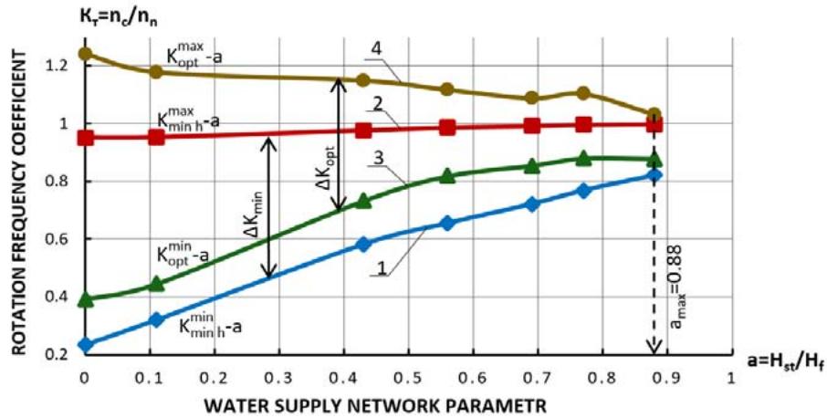 Fig. 3: The dependence of the coefficient of changing the frequent rotation of the impeller
$(\mathsf{K}_{\mathsf{T}})$ on the hydraulic factor (a) at minimizing of the excessive heads for different methods of selection of the optimal parameters of a pumping unit
The method of the selection of the pump parameters: 1, 2 — for the traditional method of selection of the optimal parameters of the pumping unit; 3,4 — for method NPL "ENERGOSIT" at the most possible load In such a case, curve 3 (see Fig. 4) shifts in respect to the X axis to position 4. The value of the Y axis of the curve shift $\Delta K$ is defined by the value of the hydraulic factor of the pipeline system (see Fig. 3). At shifting to position 4 the curve ABC crosses line 1 at the pointBwhere the frequency of rotation of the impeller of the virtual pump is equal to the nominal $(\mathsf{K}_{\tau} = 1)$ and its head is equal to the optimal $(Q_{j} = Q_{opt}^{\mathrm{virt}})$. That is why all the head modes of the pump when operating within the AB area $(Q_{\min} \leq Q_{j} \leq Q_{opt}^{\mathrm{virt}})$ will be underloading, and it is required to reduce the frequency of rotation of the impeller $(n_{C} < n_{N})$ for their support, although overloading under operation in the BC area $(Q_{opt}^{\mathrm{virt}} \leq Q_{j} \leq Q_{max})$, for which the increase of the frequency is required $(n_{C} > n_{N})$. The study of geometric shapes of the universal characteristics of the rotodynamic vane blowers in a wide range of varying rotation of the impeller from 0.5 to $1.3n_{N}$ and heads from 0.25 to $1.5Q_{opt}$ has shown that the deviation of the current frequency of rotation from the nominal towards a greater or lesser value within the limits $\pm 15\%$ ( $0.85 \leq k_{T} \leq 1.15$ ) leads to the decline of the maximal value of efficiency no more than $3 - 5\%$. At the traditional selection of the pump parameters for the maximal (peak) load $(Q_{opt} = Q_{max})$ all the operation modes of the pump relative to $Q_{max}$ are underloading, and as the heads go down to $Q_{min}$ a more significant decrease of the current frequency of rotation of the impeller is required. When selecting the pump parameters according to the most probable load while reducing cost of the virtual pump from $Q_{max}$ to $Q_{opt}^{\mathrm{virt}}$, there is an increase of the efficiency value from $\eta_{j}$ to $\eta_{max}^{\mathrm{virt}}$, and only when $Q_{j} < Q_{opt}^{\mathrm{virt}}$, its decrease begins. The shift of the value of optimal efficiency, with a maximal head inside the range of loads, i.e. in the area of the most probable heads, allows one (see Fig. 4) to reduce the deviation of the current rotation frequency of the impeller from the nominal one significantly. In the example we are examining (see Table 2) the decrease of the deviation of the current frequency from the nominal coefficient across the entire range of the load variation reduced from 19.6 (at $Q_{\mathrm{min}}$ ) up to 20.3 (at $Q_{\mathrm{max}}$ ). This circumstance provides a possibility for increasing the energy efficiency of the pumping systems' operation.
The mathematical model of the pumping system with LOWARA NSC-150-470 unit was used for the investigation of the dependence of the frequency rotation coefficient $\kappa_{\mathrm{r}}$ on the pump head for different variants of the pumping unit control. The range of variation in the flow rate of the pumping system was accepted as from $Q_{\mathrm{min}} = 140m^3 /h$ to $Q_{\mathrm{max}} = 600m^3 /h$; and the probability distribution of the flow rate was accepted the same as in the example with the WILOCronoNorm-NL-125/200 pump. The statistical head in the pipeline system was taken to be $\mathrm{asH}_{\mathrm{st}} = 20m$, the hydraulic factors $a = 0,45$, and the system hydrodynamical resistance as $\beta = 6.596 \cdot 10^{-5}(h^{2} / m^{5})$. The pump parameters selected according to the traditional methodology for the characteristic modes were: at the operation point $Q_{op} = 645m^3 /h$, $H_{op} = 47.5m$, $\eta_{op} = 0.754$; at the optimal head: $Q_{opt} = 540m^3 /h$, $H_{opt} = 54m$, $\eta_{opt} = 0.781$. The parameters of a virtual pump when selecting it according to the most probable load are as follows: $Q_{opt}^{\mathrm{virt}} = 464m^3 /h$, $H_{opt}^{\mathrm{virt}} = 34m$, $\eta_{opt}^{\mathrm{virt}} = 0.781$. The results of the $K_{\mathrm{T}}$ coefficient calculation are shown in Table 2.
Table No 2: Dependence of the Coefficient of Changes in the Rotation Frequency of the Impeller (Kc) on the Flow of the Pump for Different Control Methods
<table><tr><td>No of Parameter</td><td>1</td><td>2</td><td>3</td><td>4</td><td>5</td><td>6</td><td>7</td><td>8</td><td>9</td><td>10</td><td>11</td><td>12</td></tr><tr><td>Q, m3/h</td><td>140</td><td>180</td><td>240</td><td>280</td><td>320</td><td>360</td><td>400</td><td>440</td><td>480</td><td>520</td><td>560</td><td>600</td></tr><tr><td>Kother</td><td>1</td><td>1</td><td>1</td><td>1</td><td>1</td><td>1</td><td>1</td><td>1</td><td>1</td><td>1</td><td>1</td><td>1</td></tr><tr><td>Kstab</td><td>0.827</td><td>0.835</td><td>0.849</td><td>0.860</td><td>0.870</td><td>0.883</td><td>0.897</td><td>0.911</td><td>0.927</td><td>0.944</td><td>0.961</td><td>0.980</td></tr><tr><td>Kminh</td><td>0.560</td><td>0.580</td><td>0.618</td><td>0.646</td><td>0.677</td><td>0.711</td><td>0.746</td><td>0.784</td><td>0.823</td><td>0.863</td><td>0.905</td><td>0.947</td></tr><tr><td>Kopt</td><td>0.756</td><td>0.775</td><td>0.812</td><td>0.840</td><td>0.871</td><td>0.904</td><td>0.941</td><td>0.979</td><td>1.019</td><td>1.040</td><td>1.105</td><td>1.150</td></tr></table>
In compliance with the data from Table 2, Fig. 4 shows diagrams with dependencies of $\mathbf{K}_{\mathrm{T}} = \mathbf{f}(\mathbf{Q})$ for different ways of control. When throttling of the pipeline system takes place, the pump operates with the constant rotation frequency $\mathsf{K}_{\mathrm{T}} = 1$ (see curve 1), and when stabilizing the pressure in the pressure header (see curve 2), the values of the $\mathbf{K}_{\mathrm{T}}$ coefficient were changing within the range from 0.827 to 0.98.
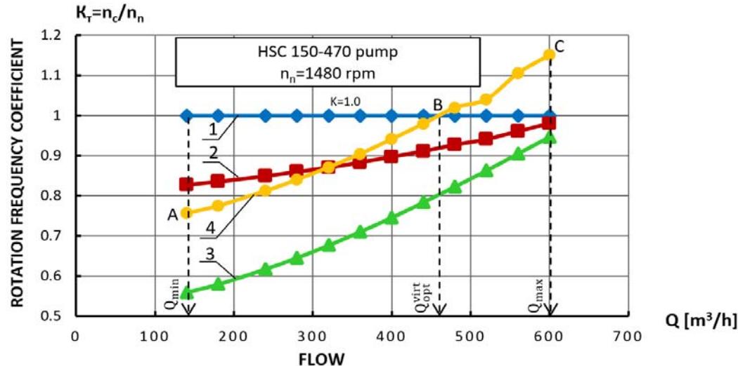 Fig. 4: Dependence of the Coefficient of Changes in the Current Rotation Frequency of the Impeller of the Pump on the Flow for Different Ways of Pump Control with Applying the Variable Frequency Drive
### Control method:
1. Throttling of a pressure header;
2. Stabilization of the pressure in a pressure header;
3. Minimization of the excessive heads;
4. Optimization of the pump parameters using the model of the virtual pump.
The dependencies of the $\mathbf{K}_{\mathrm{T}}$ coefficient for two different cases of the selection of the pump equipment are presented in Fig. 4. In the case of selecting the pump parameters by a traditional way at minimization of excessive heads (see Fig. 4, curve 3), the value of the $\mathbf{K}_{\mathrm{T}}$ coefficient varied from 0.56 (at $Q_{\mathrm{min}} = 140m^3 /h$ ) to 0.947 (at $Q_{\mathrm{max}} = 600m^3 /h$ ). When selecting the parameters at the most probable load with using a virtual pump, the values of the $\mathbf{K}_{\mathrm{T}}$ coefficient changed from 0.756 (at $Q_{\mathrm{min}}$ ) to 1.15 (at $Q_{\mathrm{max}}$ ).
In regard to the above mentioned, of interest is the study of the pump efficiency dependence on the degree of deviation of the current rotation frequency of the impeller from the nominal one, i. e. on the $\mathsf{K}_{\mathrm{c}}$ coefficient. The results of this research with the use of a mathematical model describing a pumping system with HSC-150-470 unit are given in Table 3.
Table No 3: Dependence of the Pump Efficiency on the Coefficient of Changes in the Rotation Frequency at Minimization of the Excessive Heads.
<table><tr><td>No of Parameter</td><td>1</td><td>2</td><td>3</td><td>4</td><td>5</td><td>6</td><td>7</td><td>8</td><td>9</td><td>10</td><td>11</td><td>12</td></tr><tr><td>Q, m3/μ</td><td>140</td><td>180</td><td>240</td><td>280</td><td>320</td><td>360</td><td>400</td><td>440</td><td>480</td><td>520</td><td>560</td><td>600</td></tr><tr><td>Kτ</td><td>0.560</td><td>0.581</td><td>0.618</td><td>0.646</td><td>0.577</td><td>0.711</td><td>0.747</td><td>0.784</td><td>0.823</td><td>0.863</td><td>0.905</td><td>0.947</td></tr><tr><td>η</td><td>0.387</td><td>0.463</td><td>0.553</td><td>0.600</td><td>0.540</td><td>0.673</td><td>0.700</td><td>0.721</td><td>0.739</td><td>0.752</td><td>0.764</td><td>0,768</td></tr></table>
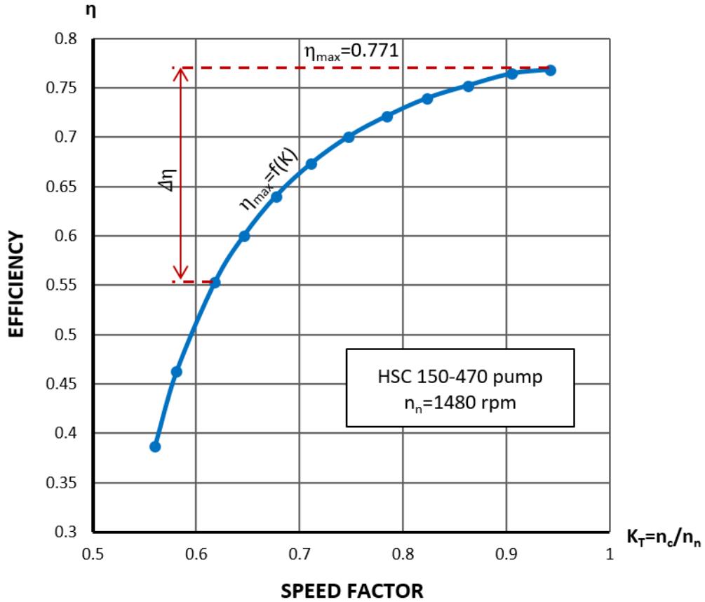
Fig. 5 displays a diagram of the pump efficiency dependence on the $\mathsf{K}_{\mathsf{T}}$ coefficient, i.e. $\eta = f(\mathsf{K}_{\mathsf{T}})$ with the use of data from Table 3.
From the given Figure and Table 3 it can be seen that with a slight reduction of the impeller rotation frequency $(0.75\leq K_{T}\leq 1)$ the dependence $\eta = f(K_{T})$ is close enough to the linear one, but with a subsequent decrease of the rotation frequency; the obtained dependence becomes exponentially vanishing. For a more detailed analysis of the efficiency characteristics dependent on the $\mathsf{K}_{\mathrm{T}}$ coefficient, consideration of the data presented in Table 4 is of certain interest.
Table No 4: Dependence of Intensity of Decrease of the Pump Efficiency on the Range of Changes in the Coefficient of Rotation Frequency of the Impeller.
<table><tr><td>No n/n</td><td>Range of changes in the coefficient of rotation frequency of the impeller Kt=nC/nN</td><td>Current value of the rotation frequency of the impeller, nC=Kr□nN</td><td>Reduction of efficiency (%) in the considered range of the coefficient Kr</td><td>Summary reduction of efficiency (%) for the current frequency nc</td></tr><tr><td>1</td><td>Kt=1</td><td>nC=nN</td><td>nT=nmax=0.771</td><td>-</td></tr><tr><td>2</td><td>0.9÷0.95</td><td>(0.9÷0.95)nN</td><td>1.0</td><td>1.0</td></tr><tr><td>3</td><td>0.85÷0.90</td><td>(0.85÷0.90)nN</td><td>2.0</td><td>3.0</td></tr><tr><td>4</td><td>0.80÷0.85</td><td>(0.80÷0.85)nN</td><td>2.0</td><td>5.0</td></tr><tr><td>5</td><td>0.75÷0.80</td><td>(0.75÷0.80)nN</td><td>2.0</td><td>7.0</td></tr><tr><td>6</td><td>0.70÷0.75</td><td>(0.70÷0.75)nN</td><td>4.0</td><td>11.0</td></tr><tr><td>7</td><td>0.65÷0.7</td><td>(0.65÷0.7)nN</td><td>4.0</td><td>15.0</td></tr><tr><td>8</td><td>0.60÷0.65</td><td>(0.60÷0.65)nN</td><td>10.0</td><td>25.0</td></tr><tr><td>9</td><td>0.55÷0.60</td><td>(0.55÷0.60)nN</td><td>14.0</td><td>39.0</td></tr></table>
It is seen from Table 4 that the entire range of changes in the $\mathsf{K}_{\mathsf{T}}$ coefficient was split into equal intervals with its variation in the limits of each interval equal to $0.05\% \cdot \mathsf{K}_{\mathsf{T}}$. The Table presents for each interval the values of the current rotation frequency, values of
Efficiency reduction in the specified intervals, as well as summary reduction of efficiency at deviation of the current value of rotation frequency from the nominal. As it has been pointed out above, at the linear segment of the curve(see Fig. 5)decrease of efficiency with variation of $\mathsf{K}_{\top}$ by $20\%$ (in the limits from 0.95 to 0.75) amounted approximately to $7\%$, while its further reduction by the same value (from 0.75 to 0.55) led to a decrease in the efficiency value by $32\%$; and the summary reduction of efficiency over the whole range of changes in $\mathsf{K}_{\top}$ amounted to $39\%$.
Thus, the parameters of pumping systems changed within a wide range when performing an investigation of the possible deviations of the impeller rotation frequency from the nominal as well as when controlling the modes of the pumps' operation. So, the possible range of current values of the $Q_{\mathrm{T}}$ flow, for instance, was in the limits from 0.25 up to $1.4$, $Q_{\mathrm{opt}}$; the variation of the hydraulic factor of the pipeline systems $(a = H_{\mathrm{st}} / H_{\mathrm{n}})$ covered practically the whole range of its possible values, that is from 0 to 0.88. At the same time, research was conducted into a broad range of variation of the impeller rotation frequency, which changed in a wide interval of possible operating modes of the pump from 0.55 up to $1.25 \, \mathrm{n}_{\mathrm{N}}$. The $K_{\mathrm{T}}$ coefficient of the rotation frequency variation is an auxiliary factor which allows one to judge indirectly about the efficiency of the pump operation, while the key factor that determines the energy efficiency of the pump operation is its efficiency coefficient. That is why the study of the certainty of determination of the efficiency values for the studied range of variation of the $K_{\mathrm{T}}$ rotation frequency coefficient is of considerable interest. The unit for determination of the pump efficiency that is a part of a computer program for estimation of the energy efficiency of the LAB-MZ pumping systems allowed us to calculate the efficiency values for different operating modes using the formulas of the hydrodynamic similarity theory and curves of similar modes (CSM) which are efficiency's equal value lines. However, in practice, as it was pointed out earlier, the efficiency constancy condition $(\eta = \text{const})$ along the CSM is fulfilled not in full, which leads to deviation of the real efficiency values from the calculated ones. Here, the values of the indicated divergence increase with the growth of the deviation of the current rotation frequency from the nominal, i.e. from the magnitude of the $K_{\mathrm{T}}$ coefficient value.
The only source of obtaining trustworthy values of efficiency under the deviation of the current rotation frequency of the impeller from the nominal one is its universal characteristics, which are received when doing bench tests of a pump with a variable rotation frequency of the impeller. Since the universal characteristics of the pump present a family of curves of complex geometric form, their practical use was most difficult up to a certain moment. The main impediment on the way to their wide application for the analysis of energy efficiency of pumping systems and control in the online mode was their transfer from the geometric form to the analytical one. The appearance over the last years of a series of specialized computer programs for digitizing curves of complex geometric form opens up a way to their practical application.
However, the availability of modern computer software for automated digitizing of single curves of complex geometric forms does not allow one to read the efficiency value from the universal characteristics representing a whole family of such curves. At the same time, the operating point of the pump shifts into the area of possible modes of its operation along the trajectory set by the selected control method.
The trajectory intersects a considerable part of the isolines, each of which corresponds to a certain level of the efficiency value. Therefore, when analyzing the online modes of the pump operation, its greater part may appear in the intervals between the digitized isolines, between which the efficiency gradient can be quite significant, especially for the isolines placed at the periphery off the center with the maximal value of efficiency.
This circumstance has required development of a specialized algorithm and compiling a computer program on its basis for calculating the efficiency with the help of pre-digitized universal characteristics of the pump. Setting up a problem is based on the visual study of examples of the universal and head characteristics of rotodynamic vane blowers, which are presented in the catalogues of manufacturing companies. For the analytical expression of the head characteristic $\mathrm{H} = \mathrm{f}_1(\mathrm{Q},\mathrm{K})$ formula 2 for the nominal rotation frequency of the impeller ( $\mathsf{K}_{\mathsf{T}} = 1$ ) was used, which was extrapolated for broadening of the region of possible modes of the pump by way of enhancing the rotation frequency by 20%, that is $\mathsf{H}_2 = \mathsf{f}_2(\mathsf{Q},\mathsf{K})$, where $\mathsf{K}_{\max} = 1.2$. The worked out algorithm was applied to the mathematical model of the WiloCronoNormNL-125/200 pump, the universal characteristics of which are given in Fig. 2. At the same time, the following conditions of the pump operation were set: the parameters of the pump at the operating point ( $\mathsf{Q}_{\mathsf{op}} = 618\mathsf{m}^3 /\mathsf{h}$, $\mathsf{H}_{\mathsf{op}} = 45.2\mathsf{m}$ ) of the optimal mode ( $\mathsf{Q}_{\mathsf{opt}} = 442\mathsf{m}^3 /\mathsf{h}$, $\mathsf{H}_{\mathsf{opt}} = 56.7\mathsf{m}$, $\eta_{\mathsf{opt}} = 0.809$ ). The statistic head of the pipeline system was taken as equal to $\mathsf{H}_{\mathsf{st}} = 26\mathsf{m}$, the hydraulic factor $\mathsf{a} = 0.56$. The stabilization pressure in the pressure header of the system was taken as follows: $\mathsf{P}_{\mathsf{stab}} = 4.6$ t.a. The range of load fluctuation was in the limits from $\mathsf{Q}_{\min} = 140\mathsf{m}^3 /\mathsf{h}$ up to $\mathsf{Q}_{\max} = 600\mathsf{m}^3 /\mathsf{h}$, the probabilities of flow distribution in the limits of the range were taken according to the statistical data.
Because of the limited volume of this publication, we will confine ourselves to a brief description of the worked out algorithm for determining the pump efficiency using the universal characteristics. The algorithm envisages the following sequence of implementing operations:
- The dimensions of the area of the set-up problem are defined visually at the universal characteristics:
$Q_{\mathrm{max}}$ $Q_{\mathrm{min}}$ and $H_{\mathrm{min}}$. Building of the area of determination begins «from the inside» from the point Z (see Fig. 2), where the maximal value of efficiency $(Q_{\mathrm{opt}}, H_{\mathrm{opt}})$ is achieved. Its coordinates are used for setting up appropriate boundaries of the region from the point of view of possible operation modes of the pump. For the pump used in the example, at specified conditions of its operation the following restrictions were set: by the X-axis — $Q_{\mathrm{min}} = 0.2Q_{\mathrm{opt}}$ $Q_{\mathrm{max}} = 1.6Q_{\mathrm{opt}}$ by the Y-axis — $H_{\mathrm{min}} = 0.2H_{\mathrm{opt}}$. The value $H_{\mathrm{max}}$ was set by its maximal value in the interval $(Q_{\mathrm{max}}; Q_{\mathrm{min}})$ according to the head characteristic of the pump (see formula 2) at $K_{\mathrm{T}} = 1.2$.
- The minimal distance between the isolines is set up by the X-axis $\Delta$. As a grid spacing the expression $(grid^{*}\Delta)$ is used, where the fineness parameter is chosen in the interval $0 < grid < 1$. In the considered algorithm the grid value was taken as equal to $2/5$; consequently, this means that between two any isolines at least two grid nodes will be placed, which leads to a reduction in the error of the approximate calculation of efficiency.
- The number of the nodes along the $X$ -axis is calculated according to the formula $N = 1 + (Q_{\max} - Q_{\min}) / \text{grid}^* \Delta$, with the round-off of the result up to an integer number.
- The position of the coordinate axes is set for digitization.
For a specific operation of the algorithm for calculation of the distances and angles on the XY plane, it is required that the grid spacing along the Y-axis be equal to the grid spacing along the X-axis. This demanded renormalization of the Y-axis with the introduction of scaling parameters: $S = (Q_{\max} - Q_{\min}) / H_{\max} - H_{\min}$. The introduction of the scaling parameter $S$ is equivalent to nondimensionalization of the system of coordinates. Renormalized coordinates $Y_{\min} = SH_{\min}$ and $Y_{\max} = SH_{\max}$ were used as the Y-axes for digitizing the isolines which were set up using the GetData Graph Digitizer program [18]
After this digitizing of the isolines in a certain order is performed, where the vectors are columns with the values for the isoline coordinates X, Y, a special matrix called "lines" can be filled in. Results of automated digitizing of the universal characteristics of the WiloCronoNormNL-125/200 pump are given in Fig.6. The result of automated digitizing is derived using the Get Data Graph Digitizer program with the distance between the points selected far smaller than the grid spacing. In the given example, the number of points, for instance, along line 1, which are placed most closely to the Z point of the maximal efficiency, is equal to 17. It should be noted that at the maximal achievable accuracy of manual digitization of the same curve at the diagram of the A4 format, the number of points equals 6, which is by three times less.
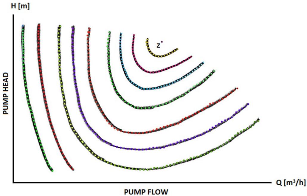 Fig. 6: Automatic Digitalizing of Universal Characteristics of the Pump WILO-CronoNorm-NL125/200 (see
Calculation of the efficiency values in the area of possible operating modes of the pump was done by the method of the "fastest descent" between the isolines of the universal characteristics. In the method of the "fastest descent", it is required to find for a given node the distance from this node to the nearest isolines between which this node is located. If the distance up to the closest isolines with the efficiencies $\eta_{1}$ and $\eta_{2}$ are equal to $d_1$ and $d_2$, respectively, then the value of efficiency can be calculated according to the formula:
$$
\eta = \frac {\eta_ {1} d _ {1} + \eta_ {2} d _ {1}}{d _ {1} + d _ {2}} \tag {8}
$$
The obtained algorithm, firstly, is a linear one and, secondly, a local one as it uses the information only about two neighbouring isolines. Herein lies its advantage, especially in the terms of this task when the number of isolines is insignificant by itself; moreover, the difference in the efficiency values between the neighbouring isolines can be quite inhomogeneous. This circumstance dramatically increases errors at the periphery when any grid algorithms are used. Formula 8 works best in the case if isolines are approximately parallel. The elaborated algorithm permits to obtain a perspective view of the surface of the efficiency values for the studied model of the pump in the R programming environment with an open source code (see Fig. 7).
The developed algorithm and computer program for reading the efficiency values with universal characteristics of the pump were included into a computation unit for its values using the LAB-MZ program for evaluation of the energy efficiency of pumping systems. Introduction of efficiency calculation into the efficiency computation unit in the LAB-MZ program for the algorithm of efficiency determination using the universal characteristics has broadened its possibilities substantially. This circumstance allows one to calculate the pump efficiency, which is necessary for the analysis of the energy efficiency of operation of pumping systems by two independent methods, namely: the traditional one using the formulas of the hydrodynamic similarity theory for vane blowers, as well as by way of pre-digitizing and reading of the actual values of efficiency from the universal characteristics of the studied pump.
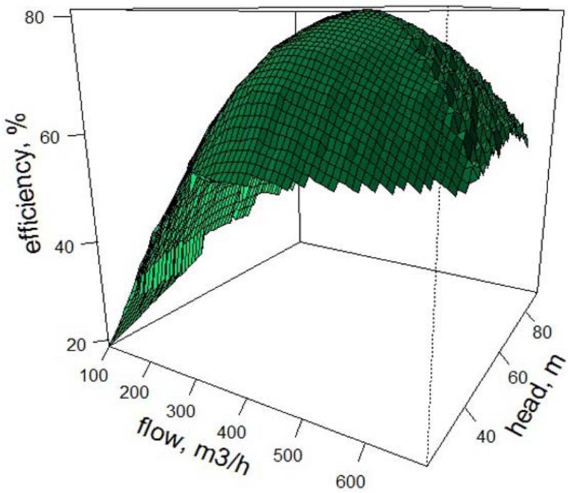 Fig. 7: A Perspective View of the Efficiency Surface
In this connection, a correlation of the efficiency values calculated by two different methods is of interest, as well as other important indices for determination of the energy efficiency during mathematical modelling of the WiloCronoNormNL-125/200 pumping unit in the case of using different control methods. Table 5 presents the energy efficient values for the following control ways: throttling of a pipeline system (pos.1), pressure stabilization in a pressure header (pos.2), minimization of excessive heads (the so-called its modification - proportional control) (pos.3), as well as minimization of the excessive heads using the universal characteristics (pos.4) by way of the transfer of the optimum of its efficiency to the point with the optimal parameters determined at the most probable load using a virtual pump $(Q_{\mathrm{opt}} = 438m^3 /h;H_{\mathrm{opt}} = 36m)$
Table 5 presents the results of calculation of the pump efficiency with the help of the formulas of hydrodynamic similarity of vane superchargers $(\eta_{\mathrm{csm}})$ and digitizing and reading the efficiency from the universal characteristic $(\eta_{\mathrm{ucn}})$, as well as their difference: $\Delta \eta = \eta_{\mathrm{csm}} - \eta_{\mathrm{ucn}}$. In the Table, the values of the coefficient of deviation of the current rotation frequency of the impeller from the nominal one and some other indices are given also.
Table No 5: Correlation of the Values of the Pump Efficiency Calculated using the Formulas of Hydrodynamic Similarity and by Way of Pre-digitizing and Reading its Values from the Universal Characteristics for Different Control Methods
<table><tr><td rowspan="2">Compared parameters for different control methods</td><td rowspan="2">Units</td><td colspan="13">Pump flow Q, m3/h</td></tr><tr><td>140</td><td>180</td><td>220</td><td>260</td><td>300</td><td>340</td><td>380</td><td>420</td><td>460</td><td>500</td><td>540</td><td>580</td><td>600</td></tr><tr><td colspan="15">1. Throttling of the pipeline system</td></tr><tr><td>Head, Hth</td><td>m</td><td>62.6</td><td>62.9</td><td>62.7</td><td>62.2</td><td>61.5</td><td>60.4</td><td>59.1</td><td>57.5</td><td>55.6</td><td>53.5</td><td>51.0</td><td>48.3</td><td>46.5</td></tr><tr><td>Required head, Hq</td><td>m</td><td>27.0</td><td>27.6</td><td>28.4</td><td>29.4</td><td>30.5</td><td>31.8</td><td>33.3</td><td>34.9</td><td>36.7</td><td>38.6</td><td>40.7</td><td>43.0</td><td>44.2</td></tr><tr><td>Supplied power</td><td>kW</td><td>55.0</td><td>58.4</td><td>61.7</td><td>65.2</td><td>68.9</td><td>72.7</td><td>76.7</td><td>81.1</td><td>85.9</td><td>91.1</td><td>97.1</td><td>104.0</td><td>107.9</td></tr><tr><td rowspan="2">Theoretical power of the coef. of rotation frequency Kr</td><td>kW</td><td>12.7</td><td>17.6</td><td>28.4</td><td>29.4</td><td>30.5</td><td>31.8</td><td>33.3</td><td>34.9</td><td>36.7</td><td>38.6</td><td>40.7</td><td>43.0</td><td>44.2</td></tr><tr><td>-/-</td><td>1</td><td>1</td><td>1</td><td>1</td><td>1</td><td>1</td><td>1</td><td>1</td><td>1</td><td>1</td><td>1</td><td>1</td><td>1</td></tr><tr><td>Coefficiency, ηcsm</td><td>%</td><td>43.6</td><td>52.9</td><td>60.9</td><td>67.5</td><td>72.9</td><td>76.9</td><td>79.7</td><td>81.1</td><td>82.1</td><td>79.9</td><td>77.3</td><td>73.5</td><td>71.1</td></tr><tr><td>Coefficiency, ηhist</td><td>%</td><td>48.1</td><td>57.9</td><td>64.0</td><td>69.7</td><td>72.6</td><td>78.0</td><td>80.3</td><td>80.9</td><td>80.9</td><td>80.3</td><td>76.9</td><td>73.7</td><td>70.9</td></tr><tr><td>Δη</td><td>%</td><td>+4.5</td><td>+5.0</td><td>+3.1</td><td>+2.2</td><td>-0.3</td><td>+1.1</td><td>+0.6</td><td>-0.2</td><td>-1.2</td><td>+0.4</td><td>-0.4</td><td>+0.2</td><td>-0.2</td></tr><tr><td>Energy consumed over one year</td><td>kW·h</td><td colspan="13">Sth=691,4thous. kW·h</td></tr><tr><td colspan="15">2. The pressure stabilization in the pressure header</td></tr><tr><td>Coef. of changes in the rotation frequencyKt</td><td>-/-</td><td>0.854</td><td>0.856</td><td>0.859</td><td>0.865</td><td>0.873</td><td>0.884</td><td>0,896</td><td>0,910</td><td>0,976</td><td>0,942</td><td>0,962</td><td>0,983</td><td>0,993</td></tr><tr><td>Coef, ηcsm</td><td>%</td><td>48.3</td><td>57.9</td><td>65.6</td><td>71.6</td><td>76.0</td><td>78.8</td><td>80.8</td><td>80.5</td><td>79.6</td><td>77.9</td><td>75.4</td><td>72.3</td><td>70.5</td></tr><tr><td>Coef, ηhist</td><td>%</td><td>42.3</td><td>52.4</td><td>59.9</td><td>66.5</td><td>71.9</td><td>75.5</td><td>76.8</td><td>77.3</td><td>76.7</td><td>75.7</td><td>73.4</td><td>71.4</td><td>70.1</td></tr><tr><td>Δη</td><td>%</td><td>-6.0</td><td>-5.5</td><td>-5.7</td><td>-5.1</td><td>-4.0</td><td>-3.3</td><td>-4.0</td><td>-3.2</td><td>-2.9</td><td>-2.2</td><td>-2.0</td><td>-0.9</td><td>-0.4</td></tr><tr><td>Energy consumed over one year</td><td>kW·h</td><td colspan="13">Sta=557,5thous. kW·h</td></tr><tr><td colspan="15">3. Minimization of excessive heads (proportional control)</td></tr><tr><td>Coef. of changes in the rotation frequencyKt</td><td>-/-</td><td>0.655</td><td>0.667</td><td>0.683</td><td>0,703</td><td>0,727</td><td>0,754</td><td>0,783</td><td>0,815</td><td>0,849</td><td>0,884</td><td>0,922</td><td>0,960</td><td>0,980</td></tr><tr><td>Coef, ηcsm</td><td>%</td><td>52.6</td><td>61.4</td><td>67.8</td><td>72.2</td><td>74.6</td><td>76.3</td><td>76.8</td><td>76.4</td><td>75.4</td><td>74.1</td><td>72.4</td><td>70.4</td><td>69.4</td></tr><tr><td>Coef, ηhist</td><td>%</td><td>27.8</td><td>39.1</td><td>48.7</td><td>55.6</td><td>60.6</td><td>64.6</td><td>67.0</td><td>69.2</td><td>69.0</td><td>69.5</td><td>69.6</td><td>69.5</td><td>69.3</td></tr><tr><td>Δη</td><td>%</td><td>-24.8</td><td>-22.3</td><td>-19.1</td><td>-16.6</td><td>-14.3</td><td>-11.7</td><td>-9.8</td><td>-7.2</td><td>-6.4</td><td>-4.7</td><td>-2.8</td><td>-0.9</td><td>-0.1</td></tr><tr><td>Energy consumed over one year</td><td>kW·h</td><td colspan="13">Stmin=443,8thous. kW·h</td></tr><tr><td colspan="15">4. Minimization of excessive heads using the universal characteristics of the pump by way of transferring its optimum of the efficiency to the point with optimal parameters determined for a virtual pump (Qvort=438m3/h; Hvort=36m)</td></tr><tr><td>Coef. of changes in the rotation frequencyKt</td><td>-/-</td><td>0.818</td><td>0.832</td><td>0.850</td><td>0.869</td><td>0.891</td><td>0.915</td><td>0.942</td><td>0.970</td><td>1.00</td><td>1.031</td><td>1.644</td><td>1.100</td><td>1,116</td></tr><tr><td>Coef, ηcsm</td><td>%</td><td>52.6</td><td>61.4</td><td>67.8</td><td>72.2</td><td>74.9</td><td>76.3</td><td>76.8</td><td>76.4</td><td>75.4</td><td>74.1</td><td>72.4</td><td>70.4</td><td>69.4</td></tr><tr><td>Coef, ηhist</td><td>%</td><td>44.2</td><td>53.6</td><td>61.9</td><td>69.0</td><td>73.9</td><td>77.7</td><td>80.0</td><td>81.1</td><td>80.6</td><td>78.7</td><td>75.1</td><td>70.9</td><td>68.5</td></tr><tr><td>Δη</td><td>%</td><td>-8.4</td><td>-7.8</td><td>-5.9</td><td>-3.2</td><td>-1.0</td><td>+1.4</td><td>+3.2</td><td>+4.7</td><td>+5.2</td><td>+4.6</td><td>+2.7</td><td>+0.5</td><td>-0.9</td></tr><tr><td>Energy consumed over one year</td><td>kW·h</td><td colspan="13">Sopt=434 thous. kW·h</td></tr></table>
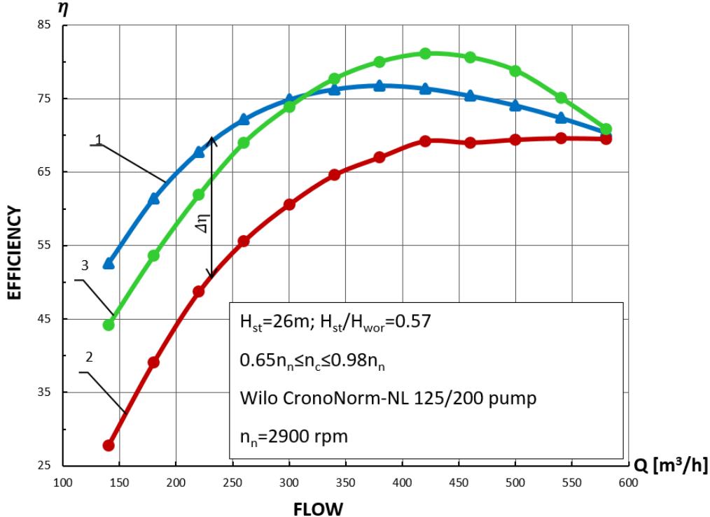
Using the data from Table 5, Fig. 8 presents diagrams with the dependences of the pump efficiency on the flow for different methods of its determination in the case when the pump is controlled by way of minimization of the excessive pressure in the pressure header of the pumping station.
 Fig. 8: Dependence of the pump efficiency on the flow for different methods of its determination when controlling the pump by way of minimization of excessive pressure in the pressure header of a pumping station (the so-called proportional control)
1. by the traditional method using the formulas of the hydrodynamic similarity theory for vane blowers;
2. using the universal (control) characteristics of the rotodynamic vane blower and traditional method of selection of its parameters;
3. using the universal characteristics of the pump by way of transfer of its optimum to the point with the parameters $\mathbf{Q}_{\mathrm{opt}}^{\mathrm{virt}}$ and $\mathbf{H}_{\mathrm{opt}}^{\mathrm{virt}}$ determined for a virtual pump.
The most substantial exceedance of efficiency calculated using the traditional technique (see Fig. 8, curve 1), from the efficiency values derived using the universal characteristics (see Fig. 8, curve 2), was obtained during minimization of excessive (above-normal) values of pressure in a pipeline system. Here, the efficiency exceedance across the entire range of changes in the flow amounted to from $1\%$ up to $23.8\%$. It should be noted that the deviation of the current rotation frequency from the nominal was, respectively, in the range from 0.98 up to 0.65 from $\mathsf{n}_{\mathsf{H}}$. The hydraulic factor of the pipeline system was equal to 0.57. It is evident that for the pumping systems with a smaller value of the hydraulic factor ( $a < 0.57$ ) the deviation of the current rotation frequency from the nominal will be more considerable and, consequently, divergence of the efficiency values computed using the formulas of similarity and with the help of the universal characteristics will be more substantial.
In Table 5 and Fig.8 (curve 3), dependence of the efficiency values read from the digitized universal characteristics of the pump is given for the case of selection of the pump parameters for the existing pipeline system using preliminary calculation of the parameters of a virtual pump $(\mathrm{Q}_{\mathrm{opt}}^{\mathrm{virt}} = 438m^{3} / h; \mathrm{H}_{\mathrm{opt}}^{\mathrm{virt}} = 36m)$. From the data provided in Table 5 (pos.4) and in Fig.8 (curve 3) it is seen that deviation of the current frequency from the nominal at coverage of the underload modes was of the order $18\%$ ( $\mathsf{K}_{\mathsf{T}} = 0.818$ ), and efficiency exceedance computed using the traditional methodology was not more than $8.4\%$ at underload modes ( $\mathsf{Q}_{\mathsf{T}} = 340\mathsf{m}^{3} / \mathsf{h}$ ). At coverage of loads in the range from 340 up to $600m^{3} / h$ the pump efficiency exceeds substantially the efficiency of a pump selected using the traditional technique (up to $5.2\%$ ) at the selection of its parameters by the most probable load. The peak load is then covered here by way of increasing the rotation frequency of the impeller by $12\%$ relative to the nominal ( $\mathsf{K}_{\mathsf{T}} = 1.116$ ).
The determining factor for making a decision concerning the reasonability of investments into the reconstruction of the acting or newly projected pumping systems is the objective evaluation of their energy efficiency. Since the pump efficiency calculation is the
 Fig. 5: Dependence of the Pump Efficiency from the Coefficient of the Rotation Frequency of the Impeller
$(\mathrm{K}_{\mathrm{r}} = n_{\mathrm{o}} / n_{\mathrm{n}})$

Fig 2) using GetData Graph Digitizer Program most significant factor that affects the trustworthiness of the value of energy efficiency of operation of pumping systems, application of the traditional methodology for its determination using the formulas of hydrodynamic similarity can lead to a significant overestimation of their energy efficiency and, consequently, to making wrong decisions about the reasonability of their construction or reconstruction.
In this connection, of interest is the correlation of the indices of energy efficiency of the modelled pumping system with the NL-125/200 pumping unit for different control methods and techniques of selecting its parameters. The energy efficiency of the pumping system on the whole and factors that determine (form) it was calculated using the LAB-MZ computer program. At the same time, the calculation of the energy efficiency was conducted taking into account the use of two variants of calculating the efficiency values, namely, using the formulas of the hydrodynamic similarity theory and by way of pre-digitizing and reading the actual values of efficiency from the universal characteristics of the pump. Results of calculation of the energy efficiency of operation of a pumping system over one year for two compared variants at different control methods are given in Table 6.
Table No 6: Comparison of the Energy Consumed by the Pump for Different Methods of Determination of its Efficiency and Control Methods
<table><tr><td rowspan="2">No</td><td rowspan="2">Method of control of a pumping unit and method of selection of the optimal parameters</td><td colspan="2">Consumed electric power for different methods of calculation of the pump efficiency Sw, thous. kW·h</td><td colspan="2">Increase of the value of consumed electric power at calculation of efficiency using the universal characteristics</td></tr><tr><td>by the formula of the hydrodynamic similarity theory</td><td>using the universal characteristics</td><td>thous. kW·h</td><td>%</td></tr><tr><td>1</td><td>Throttling of the pipeline system</td><td>691.4</td><td>691.4</td><td>0</td><td>0</td></tr><tr><td>2</td><td>Pressure stabilization in the pressure header of the pumping station</td><td>557.5</td><td>581.2</td><td>23.7</td><td>4.2</td></tr><tr><td rowspan="2">3</td><td>Minimization of excessive heads (proportional control) for different methods of selection the optimal parameters: - using the traditional method of selection by the maximal (peak) load</td><td>443.8</td><td>500.2</td><td>56.4</td><td>12.7</td></tr><tr><td>- Optimization of the parameters of the selected equipment using a virtual pump</td><td>420.1</td><td>434.4</td><td>14.4</td><td>3.4</td></tr><tr><td>4</td><td>Theoretical minimally possible energy consumption (minimum of the energy functional)</td><td>405.7</td><td>405.7</td><td>0</td><td>0</td></tr></table>
It is visible from the data provided in Table 6 that the use of the formulas of hydrodynamical similarity for the calculation of efficiency of the pump leads to an overestimation of the expected energy efficiency of its operation. Thus, for instance, at pressure stabilization in the pressure header the exceedance of energy efficiency calculated using the formulas of hydrodynamic similarity was $4.2\%$, while at minimization of the excessive heads the exceedance of the calculated energy efficiency increased up to $12.7\%$. At pressure stabilization, as has been pointed out earlier, deviation of the current rotation frequency from the nominal was insignificant and amounted to $15\%$, increased up to $35\%$ at minimization of the excessive heads, which entailed overestimation of the calculated energy efficiency up to $12.7\%$. That is why, broadening of the flow range (at pressure stabilization) or further decrease of the static component of the required head of the pipeline system (at the minimization of the excessive heads) will lead to a more substantial exceedance of the calculated efficiency relative to the actual one obtained through computation of the efficiency by way of using the universal characteristics of the pump.
As can be seen from Table 6, the largest energy effect is achieved in the case of the maximal binding of the characteristics of the installed pump to the parameters of the network by way of selection of the pump by the most probable load using a virtual pump. The transfer of the optimum of the efficiency of the selected pump to the point with optimal parameters obtained for a virtual pump $(\mathbf{Q}_{opt}^{\mathrm{virt}}$ and $\mathbf{H}_{opt}^{\mathrm{virt}})$ allows one to achieve the maximal yearly energy efficiency $(S_{w} = 434$ thousand kW*h) which ensures the maximal (up to $90\%$ extraction of the energy saving potential, which is not permitted by any of the known methods.
## II. MAIN CONCLUSIONS
1. The question about reduction of the pump efficiency at deviation of the current rotation frequency of the impeller $(n_{\mathrm{T}})$ from the nominal $(n_{\mathrm{H}})$ had theoretical interest during a long time and was brought into the practical plane only with broad application of the variable-frequency drive. Regulation of the operating modes of the pump by way of changing the rotation frequency of the impeller leads to a change of its parameters: head, flow and efficiency, which requires recalculation of its characteristics from the nominal to the current rotation frequency. In connection with the violations of the conditions of hydrodynamic similarity at change of the frequency rotation, the greatest difficulties appear after recalculation of the efficiency of the rotodynamic vane blower, for which formulas of hydrodynamic similarity are traditionally used. The requirements of the Euro-zone standards to the minimally allowed value of the efficiency index (MEI) cover only a rather narrow part of the area of possible modes of the pump operation in the range of flows that are close to the optimal (from 0.75 up to $1.1Q_{\mathrm{opt}}$ ). Due to the narrowness of the range of modes covered by the standard, the deviations of the current frequency from the nominal in this range will be in significant (no more than $10 - 15\%$ ), but in the frequently occurred in practice cases of the substantial widening of the load range (from 0.25 to $1.2Q_{\mathrm{opt}}$ ) as well as in the case of applying more energy efficient ways of the pumping unit control (such as minimization of the exceeded heads or its variety – proportional regulation) will bring more significant deviations of the current rotation frequency from the nominal one. This circumstance will lead to the substantial decrease of the pump efficiency at the underload modes $(Q_{\mathrm{j}} < 0.75Q_{\mathrm{opt}})$ that can level the efficiency of the pump operation entirely at covering the whole range of heads.
2. In order to obtain numerical values of the impact of deviation of the current frequency of the impeller from the nominal $(\mathsf{K}_{\mathrm{T}} = \mathsf{n}_{\mathrm{C}} / \mathsf{n}_{\mathrm{N}})$ on the pump efficiency, the specialized LAB-MZ computer program was used, which was developed by the authors at the SPL "Energosit" (Moscow) earlier and then substantially complemented. This computer software has been designed for evaluation of the energy efficiency value of the pumping systems operating with variable load. One of the distinctive features of the LAB-MZ program is the mathematical model of the water flow process in the pipeline system. This model consists of a number of statistical intervals with distribution of the probabilities of the flows in the statistical selection, which ensures a rather full adequateness of the model and physical process of the water flow. The presence of a sufficient number of statistical intervals provides a possibility to obtain minor gradients in each of them for such important parameters forming the current value of the energy efficiency as: efficiency, head, effective and supplied power, rotation frequency of the impeller, and its deviation from the nominal. This circumstance allows one to calculate the current values of the above listed parameters, as well as the energy efficiency of the pump operation in each interval. The total index of the energy efficiency of the system is considered as a sum of its values in the entire range of the load change. Besides, LAMMZ contains an optimization unit, which executes selection of the pump equipment not by the traditional comparison of the manufactured pumps in the industry but by way of calculating the parameters of the virtual pump model by the most probable load. Then, basing on the parameters obtained for the virtual pump, a real pump with the parameters that are most close to the virtual one is selected. This is done to achieve a rather full compliance of the pump characteristics and parameters of the system, which ensures its maximal energy efficiency that cannot be achieved with the traditional method of selecting the parameters by the single operating point specified by the consumer.
3. The studies of the influence of deviation of the current rotation frequency from the nominal have been conducted on the basis of mathematical modelling of a pumping system with the NL125/200(WILO) unit for a broad flow range (from 0.25 up to $1.4\mathrm{Q}_{\mathrm{opt}}$ ) and a full spectrum of variation of the hydraulic factor a (from 0 up to 0.88, where $\alpha = H_{st} / H_{op}$ ). Research has been done for different methods of control of a pumping unit. The values of deviation of the current frequency from the nominal for pressure stabilization in the pressure header were in the range from 0.856 up to $0.996n_{N}$. A full-scale study of a whole number of objects of water supply systems has shown that in practice there are often cases when the deviation of the current frequency from the nominal at stabilization is more substantial, from 0.55 up to $0.6n_{N}$, which leads to the pump operation with the efficiency not more than 20-30%. Of the greatest interest are the results of the study of the deviation of the current frequency from the nominal at the minimization of excessive (above the normative) heads (the so-called proportional control). Here, the most considerable in its value deviation is observed, especially in the area of underload modes at an insignificant statistical constituent of the required head $H_{st}$. At minimization of excessive heads the deviation of the current frequency from the nominal was in the limits from


$0.235\mathsf{n}_{\mathsf{N}}$ (at $\mathsf{a} = 0$ ) up to $0.821\mathsf{n}_{\mathsf{N}}$ (at $\mathsf{a} = 0.88$ ), while during selection of a pump by the most probable load the minimal value of deviation was from $0.392\mathsf{n}_{\mathsf{N}}$ (at $\mathsf{a} = 0$ ) up to 0.878 (at $\mathsf{a} = 0.88$ ). Since at determination of parameters using a virtual pump underload modes were covered by reduction of the rotation frequency, and maximal flows by way of its increasing in respect to the nominal, the value of the current frequency for the virtual pump was from $1.22\mathsf{n}_{\mathsf{N}}$ (at $\mathsf{a} = 0$ ) up to $1.032\mathsf{n}_{\mathsf{N}}$ (at $\mathsf{a} = 0.88$ ). At the minimization of excessive heads for the HSC-150-470 pump, the pump efficiency dependence on the degree of deviation of the impeller frequency from the nominal was obtained, which was in the interval from 0.56 up to $0.942\mathsf{n}_{\mathsf{N}}$ in the tests. Analysis of the dependence $\eta = \mathsf{f}(K_T)$ has shown that at insignificant deviations of $K_{T}$ in the range from 1.0 up to $0.8\mathsf{n}_{\mathsf{N}}$ it is practically linear, while at further increase of the deviation the dependence becomes considerably nonlinear. If at decrease of the rotation frequency by $20\%$ (from 1.0 up to $0.8\mathsf{n}_{\mathsf{N}}$ ) the efficiency reduction amounted to $7\%$ only, while at its further decrease by the same value ( $20\%$ ) the efficiency reduction was $32\%$, and the total reduction of efficiency in the linear and nonlinear areas amounted to $39\%$ (at $\mathsf{n}_{\mathsf{T}} = 0.56\mathsf{n}_{\mathsf{N}}$ ).
4. The only source of trustworthy information about the actual values of the efficiency of the pump operating with variable rotation frequency of the impeller is its universal (control) characteristics obtained by way of conducting bench tests of pumps at different rotation frequencies of the impeller. The isolines of efficiency of equal value that are given at the universal characteristics of the pump are elliptic and oval curves located concentrically relative to the point with the maximal value of efficiency in the H-Q coordinate system. A simple visual analysis of the efficiency characteristics by way of comparing the curves of similar modes presenting a family of parabolas, which follow from the formulas of hydrodynamic similarity, and the isolines of efficiency of equal level given at the universal characteristics of the pump allow one to find out the substantial qualitative difference for the same types of pumps. This circumstance required performing special research aimed at deriving numerical difference of efficiency values obtained using the formulas of similarity and read out from the universal characteristics of the pumps for a broad spectrum of variation of the parameters of water supply systems and methods of controlling the pumping equipment. Making the required comparison is possible only in the presence of special mathematical models, algorithms and computer programs, which allow us to obtain calculated data for such a comparison.
5. The main impediment on the way to a wide application of the universal characteristics for the mathematical modelling of pumping systems with the goal of determination of their energy efficiency and the use of control of pumping units in the systems is their transfer from the geometric form to the analytic one. The appearance in the last years of a number of specialized computer programs for automatized digitizing of curves of geometric shapes opens up a way to their practical application. However, the availability of such programs does not yet ensure a possibility of reading out the efficiency values from the universal characteristics. Solving this task has required elaboration of a special algorithm and compiling a computer program that permits to read out the efficiency values independently of the trajectory of motion of the operating point of the pump in the area of possible modes of its operation. For automatized digitizing we used the GetData Graph Digitizer program. Calculation of the efficiency values with reading its values from the universal characteristics is performed using the developed algorithm at the displacement of the operating point in the H-Q coordinates for any trajectory specified by the selected method of controlling the pump. The elaborated algorithm allows one to obtain a perspective view of the surface of the efficiency of the studied pump model in the R programming environment (programming language).
6. The elaborated algorithm and computer program for reading the efficiency values from the universal characteristics of the pumps were included into the unit for computing efficiency values using the LAB-MZ program that was considered earlier. This allowed us to calculate the efficiency of the pumps and to evaluate the energy efficiency of operation of pumping systems by two independent methods - using formulas of hydrodynamic similarity and by way of reading the actual values of efficiency from the universal characteristics after their pre-digitizing. Correlation of the efficiency values and energy efficiency indices was done by mathematical modelling of the Wilo-CronoNormNL-125/200 pumping unit for different control methods and technological conditions of its operation. The analysis of comparison of the efficiency values calculated by two different methods has shown a steady tendency towards exceeding the efficiency values derived according to the formulas of hydrodynamical similarity and by way of reading its values from the universal characteristics. Since exceedance of the efficiency values calculated based on the formulas of similarity over the values read out from the universal characteristics achieves its maximal value at the pump operation in underload modes and with a relatively insignificant
static constituent of the required head, consideration of these modes with considerable deviation of the current rotation frequency of the impeller from the nominal presents the greatest interest. So, for instance, at pressure stabilization in the pressure header deviation of the current rotation frequency from the nominal amounted to $n_{\mathrm{C}} = 0.85n_{\mathrm{N}}$, and exceedance of efficiency by the similarity formulas was $5\%$. At the minimization of excessive (above norm) heads the deviation of the current frequency from the nominal was $n_{\mathrm{T}} = 0.65n_{\mathrm{H}}$ and exceedance by the similarity formulas achieved $23.8\%$. At the same time, the value of the hydraulic factor was taken as equal to $a = 0.57$. It is evident that for pumping systems with the least value of the hydraulic factor the required exceedance will be more substantial. Overestimation of the energy efficiency value of the pumping system on the whole due to the overestimation of efficiency at pressure stabilization amounted to $5.3\%$ and to $12.7\%$ at minimization of excessive heads. The obtained values of overestimation of the energy efficiency when traditional methods of efficiency determination are used testify to the necessity of using for estimation of the energy efficiency of pumping systems the efficiency values read out from the universal characteristics. This will allow us to objectively assess the energy efficiency of the pumping equipment proposed for installation (or existing) one in order to prevent adoption of insufficiently justified and wrong decisions about reasonability of investment both into reconstruction of the existing and construction of new pumping systems.
7. In the current time the universal characteristics of rotodynamic vane blowers are used chiefly for manual correction of efficiency at correction of the impeller diameter in the selected pump. The use of the universal characteristics for compiling universal algorithms for automatized reading the efficiency values at the evaluation of the energy efficiency of the pumping unit operation and selection of efficient methods of control of pumping systems revealed the necessity of enhancing the quality of the universal (control) characteristics, namely:
- Broadening of the area of coverage by the isolines of the efficiency of equal value, which are currently concentrated around the centre with the coordinate $(Q_{\mathrm{opt}}$ and $H_{\mathrm{opt}})$. Broadening at the flow shall be from 0.25 up to $1.4Q_{\mathrm{opt}}$; by the head — from 0.25 up to $1.2H_{\mathrm{opt}}$, by the impeller rotation frequency — from 0.5 up to $1.25n_{\mathrm{N}}$.
- Decrease of distance between the isolines placed at the periphery from the centre with the coordinates $(Q_{\mathrm{opt}}$ and $H_{\mathrm{opt}})$; the isolines of the constant efficiency value shall cover the area of possible modes of the pump operation fully enough and evenly; differences of the efficiency gradients between two neighbouring isolines shall not differ substantially at the periphery and at the centre of the characteristics.
- The complete set of the pumping equipment released by a manufacturing company shall contain the universal characteristics, requirements to the quality that are to be determined by the standard. This standard must be worked out in the nearest time.
(2016). Pumps. Minimum required efficiency of rotodynamic water pumps.
(2015). DIN EN ISO 14414:2019-09, Energetische Bewertung von Pumpensystemen (ISO/ASME 14414:2019); Deutsche Fassung EN_ISO_14414:2019.
(2019). DIN EN ISO 14414:2019-09, Energetische Bewertung von Pumpensystemen (ISO/ASME 14414:2019); Deutsche Fassung EN_ISO_14414:2019.
(2015). Energy conservation standards for pumps.
(2013). Enhancing energy efficiency of utilizing waste heat in heat pumps.
K Pfleiderer (1937). Centrifugal and propeller pumps.
I Sarbu,I Borza (1998). Energetic optimization of water pumping in distribution systems.
A Marchi,A Simpson,N Ertugrul (2012). Assessing variable speed pump efficiency in water distribution systems.
V Nikolaev (2008). Influence of selection of the method of control of a vane pump on the determination of its optimal parameters at variable load.
V Nikolaev (2006). Analysis of the energy efficiency of different methods of control of pumping facilities with variable drive.
V Nikolaev (2008). Energy saving methods of controlling the operating modes of a group of vane pumps operating in parallel.
V Nikolaev,G Nikolaev (2021). Updating of the criteria of the energy efficiency of pump operation, the method of choosing of their optimal parameters and control methods.
(2018). Europump guides the European Commission.
V Nikolaev,G Nikolaev (2022). Improvement of the Procedures for Assessing the Energy Efficiency of Pumping Systems.
No ethics committee approval was required for this article type.
Data Availability
Not applicable for this article.
How to Cite This Article
Valentin G. Nikolaev. 2026. \u201cThe use of Universal (Control) Characteristics of Vane Blowers for an Objective Assessment of the Energy Efficiency of Pumping Systems\u201d. Global Journal of Research in Engineering - A : Mechanical & Mechanics GJRE-A Volume 23 (GJRE Volume 23 Issue A4).
Explore published articles in an immersive Augmented Reality environment. Our platform converts research papers into interactive 3D books, allowing readers to view and interact with content using AR and VR compatible devices.
Your published article is automatically converted into a realistic 3D book. Flip through pages and read research papers in a more engaging and interactive format.
Our website is actively being updated, and changes may occur frequently. Please clear your browser cache if needed. For feedback or error reporting, please email [email protected]
Thank you for connecting with us. We will respond to you shortly.