I. INTRODUCTION

a) The problem considered and the motivation for the research

Since proteins are obtained by folding a chain of basic blocks (i.e., amino acids), there are restrictions on the shapes they can take. This means that, by observing their shapes from the outside, we should be able to make some guesses as to how the chains are folded inside. In this paper, we consider the problem using a simple mathematical model proposed in $[1]$, and present two approaches: the previous differential geometric approach and a new category theoretical approach. The author is unaware of similar studies by other researchers. Using the same category theoretical approach, the author has considered the defining equations of proteins in $[2]$. Knowledge of category theory is not required.

Proteins often interact with other molecules in the concave areas of their surface. On the other hand, the shape of the areas depend on their internal structure as mentioned above. Therefore, it is important to investigate the dependence between the surface and the internal structure of proteins.

Until now, the structural analysis of proteins has been carried out mainly by biologists who are familiar with the structures of various molecules. This reminds me of the history of cryptography. That is, many of the cryptographers of the past were linguists who knew a lot of languages. Then, William Friedman realized that mathematics would be useful in cryptography and hired many mathematicians $[4]$. The

Multiple sheets of regular flows motivation for this study is to explore the usefulness of mathematical approaches in the field of protein structure analysis.

b) The

In our model, protein molecules are represented as closed trajectories of n-simplices. For simplicity, we will only consider the case where n = 2. Closed trajectories of 2-simplices are then referred to as loops of triangles.

Ref

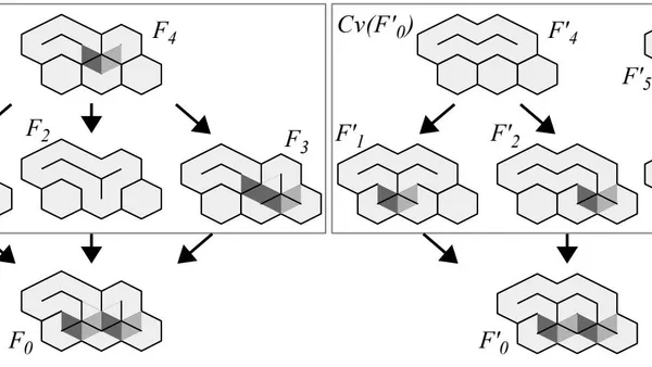
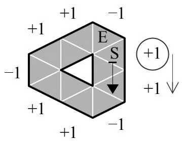
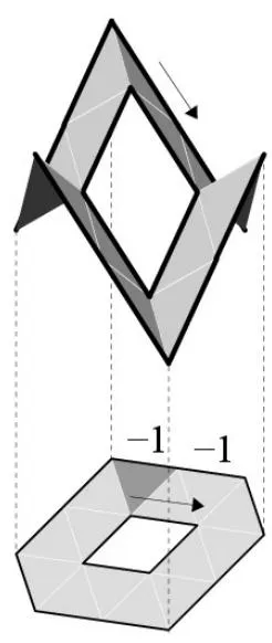
Figure 1 illustrates the two approaches using a simple example (Figure 1 (a)). As you can see, there is an "isolated" triangle inside the loop. In the previous approach proposed in [1] and [3], we examine the outer contour of a loop to detect the presence of singular triangles inside. Specifically, the "pitch" of a loop is calculated as follows. First, divide the outer contour into a set of edges of triangles. Then, moving clockwise, assign either "+1" or "-1" to each edge of the contour. The rule of assignment is "change the sign if the direction of the edge changes". The "pitch" of a loop is then defined as the sum of all the "+1"s and "-1"s assigned.

In this example, the outer contour of the loop is made up of 9 edges. First, select the starting edge (S in Figure 1 (a)) and assign it "+1". Then, move down and assign "+1" again to the adjacent edge. This is because the direction of the edge is the same as the previous one. Move down further and assign "-1" to the next edge. This is because the direction of the edge is different from the previous one. In this way, we get a sequence of "+1"s and "-1"s, as shown in Figure 1 (a). Adding up all the "+1"s and "-1"s, we obtain the "pitch" of the loop:

(a)

(b)

(c) Figure 1: Comparison of the previous approach and the new approach. (a) A loop of triangles around an "isolated" triangle. (b) A schematic view of the previous differential geometric approach. (c) A schematic view of the new category theoretical approach.

It is easy to show that the pitch will be zero if there are no singular triangles (such as "isolated" triangles) inside. Therefore, we now know that there are singular triangles inside the loop.

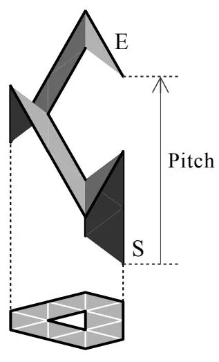
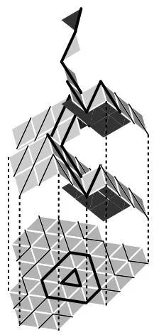
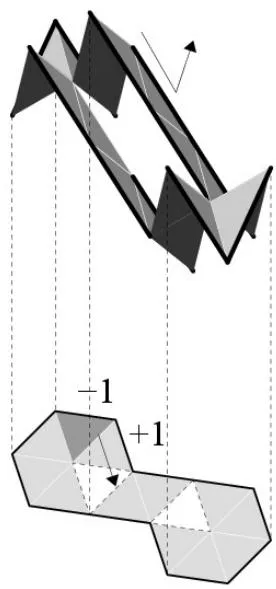
Shown in Figure 1 (b) is the mechanism of the calculation. Note that each "flat" triangle in the loop has three different directions (the lower part of the figure). Correspondingly, there are three types of "slant" triangles with different tilt directions (the upper part of the figure). Each "flat" triangle is assigned a "slant" triangle, depending on the direction of the loop at the triangle. The loop is then lifted to a trajectory of "slant" triangles in a three dimensional space. As you can see, "+1"s (resp. "-1"s) assigned to the loop correspond to the ascent (resp. descent) along the lifted trajectory. In particular, the pitch of a loop is nothing but the pitch of the lifted trajectory, i.e., the pitch of a spiral of "slant" triangles.

c) The new category theoretical approach

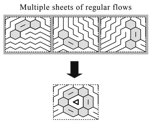
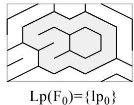
On the other hand, in the new approach proposed in this paper, we consider a set of loops that encloses a given loop (Figure 1(c) below). In this example, the given loop is enclosed by six loops. We then embed as many loops of the six enclosing loops as possible in a "regular" flow (i.e., a flow without "singular" triangles). However, it is not possible to embed all of them into a "regular" flow at once if there is a "singular" triangle inside. That is, we need multiple sheets of "regular" flows.

The "multiplicity" of a loop is the minimum number of sheets of "regular" flows required to embed all enclosing loops. In this case, three "regular" flows are required to embed the six enclosing loops (Figure 1 (c) above). On the other hand, it is easy to show that the "multiplicity" of a loop will be one if there are no singular triangles inside. Therefore, we see again that there are singular triangles inside.

Remark. In a flow of triangles, a singular loop causes a turbulence in the flow around itself, which can be detected by considering the "pitch" or the "multiplicity" of the loop. In physics, on the other hand, a particle causes a distortion in the space-time around itself. That is, the "pitch" measures the "mass" of a loop, and the "multiplicity" measures the "distortion" of the flow.

d) About this paper

In what follows, the author tries to present the two approaches outlined above in a self-contained manner using simple examples. The rest of the paper is organized as follows. Section 2 gives a brief description of Category theory. Section 3 gives a brief review of the previous approach. Section 4 gives an introduction to the new approach proposed. Section 5 summarizes our main results. Finally, Section 6 presents discussion and some suggestions for future research.

(b) Figure 2: Flow of triangles: (a) The base space $B$. (b) Regular and singular triangles. (c) A singular vector field on $B$. (Normal edges are shown as thick black lines.)

(c)

Ref

II. ABOUT CATEGORY THEORY

Category theory is the language of mathematics, appearing almost everywhere and often being a natural approach to a deeper understanding of mathematics $[5,6,7]$. Before the advent of categories, we were used to dealing with sets that had a given structure and studying their properties. On the other hand, in Category theory, the stress is placed not upon the structure of objects, but on the relations between objects within the category. In our case, the focus is on relations between proteins rather than structures of proteins.

A "category" is an embarrassingly simple concept $[7]$. In category theory, a mathematical system (i.e., a "category") is represented by a diagram of arrows. Each vertex represents an "object" of the category. Each arrow represents a "relation" between two objects. The properties of the objects of the category are then represented as properties of the diagram. The strength of this language lies in its ability to unify various branches of mathematics and to create unexpected links between seemingly different subjects.

III. THE DIFFERENTIAL GEOMETRIC APPROACH

a) Flow of triangles

To define flows of triangles, we first define trajectories of triangles. Roughly speaking, trajectories of triangles are obtained by connecting adjacent triangles by their common edge (Figure 1 (a)).

We start with the definition of the space of triangles, on which we define flows of triangles. We denote by $E^n$ the n-dimensional Euclidean space.

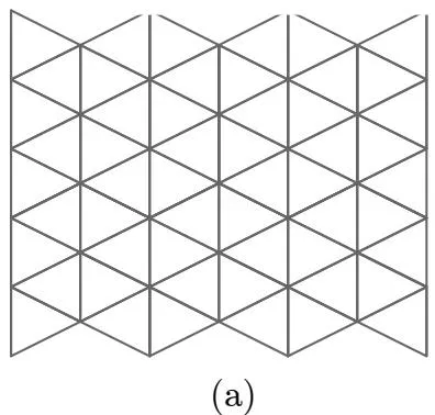
Definition 3.1 (The base space B of triangles). The base space B is the set of the triangles obtained by dividing $E^2$ into triangles. As shown in Figure 2 (a), the partitioning is done along an equilateral triangular lattice. Note that the vertices of each triangle are not contained in the interior of the edges of other triangles.

Triangles of B have a relative positional relationship due to the underlying lattice structure. To specify connections between triangles at a given triangle, we define a discrete version of the "normal vector" at the triangle.

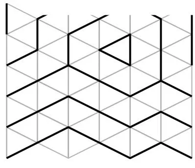
Definition 3.2 (Normal edge). Given a triangle $b\in B$. A normal edge of b is an edge of b through which b is not connected to any other triangle. In other words, adjacent triangles are connected if their common edge is not a normal edge. In the figures, normal edges are shown as thick black lines (Figure 2 (b)). Note that triangles of B may have more than one normal edge. We denote by $N(b)$ the set of normal edges assigned to $b\in B$.

Using normal edges, trajectories of triangles are defined as follows.

Definition 3.3 (Trajectory of triangles). Let $I=[0,\overline{I}]$ be an integer interval. Let

Notes be a series of triangles. Suppose that triangles $b[i](i\in I)$ are assigned normal edges. Then, T is called a trajectory in B if each successive pair has a common edge that is not a normal edge, i.e.,

for all $i,i+1\in I$. A trajectory is called closed if $b[l]$ and $b[0]$ have a common edge that is not a normal edge. Closed trajectories are simply referred to as loops. A trajectory is called open if it is not closed. A trajectory is called maximal if it cannot be made any longer. Loops are maximal.

Definition 3.4 (Regular and singular triangles). Triangles are called regular if they have exactly one normal edge. A regular triangles is connected to two adjacent base triangles (Figure 2 (b)). Triangles are called singular if they are not regular. Triangles with no normal edges are called branch triangle. They are connected to all three adjacent triangles. Triangles with two normal edges are called terminal triangle. They are connected to only one adjacent triangle. Triangles with three normal edges are called isolated triangle. They are not connected to any other triangles.

(0,y,0)

Example 3.5. Figure 1 (a) shows a loop of length 12 around an isolated triangle.

Flows of triangles are obtained by assigning normal edges to all triangles of B. We denote by PQR the triangle with vertices P, Q, and R. The three edges of PQR are then denoted by PQ (or QP), QR (or RQ), and RP (or PR).

Definition 3.6 (Vector field of triangles). A vector field V on B is an assignment of normal edges to all triangles of B, i.e., for any $PQR\in B$,

A vector field V is called singular if there is $b\in B$ such that $V(b)$ contains more than one normal edge. A vector field is called regular if it is not singular.

Example 3.7. A singular vector field is shown in Figure 2 (c).

Definition 3.8 (Flows of triangles). Let V be a vector field on B. By connecting all pairs of adjacent triangles by their common edges not in V, we obtain a set of trajectories in B. We call them the flow (of triangles) in B defined by V. A flow is called singular if the corresponding vector field is singular. A flow is called regular if the corresponding vector field is regular.

Ref

Example 3.9. The vector field of Figure 2 (c) defines a flow that includes the loop of Figure 1 (a).

b) Flow of lifted triangles

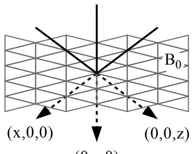
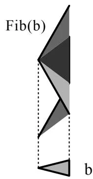
By lifting trajectories in B to trajectories in a three-dimensional space, we can compute flows in B instantly $[1]$. Moreover, we can characterize loops in B using the pitch of the corresponding spiral trajectory in the three-dimensional space. To lift trajectories upward, we first place B on the plane

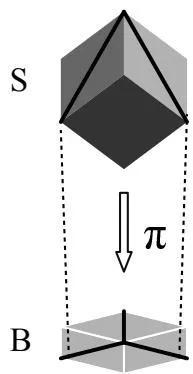
as shown in Figure 3 (a). We then stack three-dimensional unit cubes diagonally over B (i.e. in the direction from $(+\mathrm{\infty },+\mathrm{\infty },+\mathrm{\infty })$ to $(-\mathrm{\infty },-\mathrm{\infty },-\mathrm{\infty })$ ). Note that only three faces of a unit cube are visible from $(-\mathrm{\infty },-\mathrm{\infty },-\mathrm{\infty })$ (Figure 3 (b)). We call the three faces the upper faces of the unit cube. We denote by $\pi$ the diagonal projection from $E^8$ onto $B_0$, i.e.,

The three-dimensional integer lattice $Z^3$ are projected onto the set of all vertices of triangles in B by $\pi$.

Definition 3.10 (Slant triangles). Slant triangles are the triangles obtained by dividing the upper faces of a unit cube by their vertical diagonal lines. That is, a slant triangle is composed of two edges of a unit cube and the vertical diagonal of an upper face of the unit cube (Figure 3 (b)). We denote by S the set of all slant triangles. S is projected on B by $\pi$, i.e.,

Notes

(a)

(b) Figure 4: Flows in S defined by vector fields on B. (a) A singular flow in S (left) defined by the vector field on B (right). In the right figure, triangles are painted according to the direction of their normal edges. (b) A regular flow in S (left) defined by the vector field on B (right).

Remark. To distinguish between the triangles of B and the lifted triangles of S, we often refer to the former as base triangles or flat triangles.

Example 3.11. By dividing the three upper faces of a cube by the vertical diagonals, we obtain six slant triangles. The six slant triangles are then projected onto a hexagonal region of $B_0$ consisting of six base triangles (Figure 3 (b)).

Definition 3.12 (Fiber space of slant triangles over a base triangle). Let $b\in B$. The fiber space $\text{Fib}(b)$ of slant triangles over $b$ is defined by

(Figure 3 (c)).

Definition 3.13 (The normal edge of slant triangles). Let $s\in S$. The normal edge of s is the edge that corresponds to the vertical diagonal. In the figures, normal edges are shown as thick black lines. Unlike triangles of B, the normal edge of s is uniquely determined by its slope (Figure 3 (b)). We denote by $N(s)$ the normal edge of s. We denote by $\pi (N(s))$ the corresponding edge of $\pi (s)\in B$ i.e.,

where $s=PQR\in S$ and $N(s)=PQ$.

Remark. Let $s\in S$ and $b\in B$. $N(s)$ is an edge, but $N(b)$ is a set of edges. Using normal edges, trajectories in $S$ are defined in the same way as trajectories in $B$.

Definition 3.14 (Trajectory of slant triangles). Let $I=[0,I]$ be an integer interval. Let

be a series of slant triangles. Then, T is called a trajectory in S if each successive pair has a common edge that is not a normal edge, i.e.,

for all $i,i+1\in I$. A trajectory is called closed if s[0] and s[l] have a common edge that is not a normal edge. Closed trajectories are simply referred to as loops. A trajectory is called maximal if it cannot be made any longer. Loops are maximal.

Let $T=\{s[i]\Vert i\in I\}$ be a trajectory in $S$, where $I$ is an integer interval. Let $\pi (T)$ be the image of $T$ by $\pi$, i.e.,

Normal edges are then assigned on $\pi (T)$ by

Example 3.15. In Figure 1 (b), an open trajectory in S (above) is projected on a loop in B (below).

Example 3.16. Let $PQR\in B$ be an isolated triangle. $\text{Fib}(PQR)$ gives a maximal open trajectory in $S$ over $PQR$ (Figure 3 (c)), i.e.,

Definition 3.17 (Flows of slant triangles). Let $F_S$ be a set of maximal trajectories in $S$, i.e.,

where $K$ and $I_k$ ( $k\in K$ ) are integer intervals. The fiber ${\mathrm{Fib}}_{F_S}(b)$ of $F_S$ over $b\in B$ is defined by

$F_S$ is called a flow in $S$ if $Fi{b}_{F_S}(b)$ is defined for all $b\in B$.

Definition 3.18 (Vector field induced by flows in $S$ ). Let $F_S$ be a flow in $S$. The vector field induced on $B$ by $F_S$ is defined by

for $b\in B$

Definition 3.19 (Flow in S defined by a vector field on B). Let V be a vector field on B. Let $F_B$ be the flow in B defined by V. By lifting the trajectories of $F_B$, we obtain a flow $F_S$ in S. $F_S$ is called a flow in S defined by V.

Example 3.20. In Figure 4 (a), a flow in S (left above) is defined by the vector field in B on the right. The flow is spiraling around the fiber over the isolated triangle in B. The flow in S has no loop.

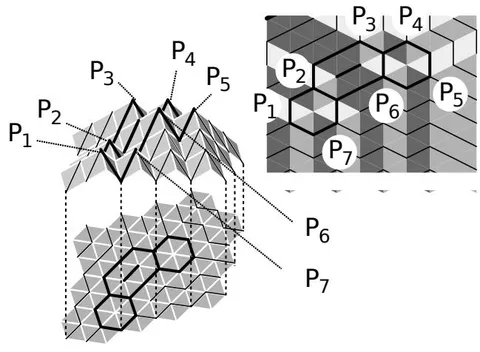
Example 3.21. In Figure 4 (b), a flow in S (left above) is defined by the vector field in B on the right. The flow in S has three loops. As you can see, the flow in S forms a "mountain range" like shape. In particular, by piling up unit cubes diagonally in $E^8$, we obtain a flow in S.

Definition 3.22 (Affine flow of slant triangles). Let M be a union of triangular cones obtained by piling up unit cubes in $E^8$ in the direction from $(+\mathrm{\infty },+\mathrm{\infty },+\mathrm{\infty })$ to $(-\mathrm{\infty },-\mathrm{\infty },-\mathrm{\infty })$. If we give the set of top vertices of the cones, M is uniquely determined. Note that only the slant triangles on the surfaces of M are visible from $(-\mathrm{\infty },-\mathrm{\infty },-\mathrm{\infty })$. The Flow in S defined on the surfaces of M are called the affine flow in S defined by M.

Example 3.23. Figure 4 (b) above is an affine flow in S defined by seven triangular cones.

Definition 3.24 (Affine flow of base triangles). Let M be a union of triangular cones. A regular flow in B is obtained by projecting the affine flow in B defined by M by $\pi$. The regular flow in B is called the affine flow in S defined by M. The corresponding regular vector field is called the affine vector field on B defined by M. A flow in B is called locally affine if it is obtained by pasting together regions of affine flows in B.

Proposition 3.25. For each loop $L_B$ in an affine flow in $B$, there is a loop $L_S$ in $S$ such that $\pi (L_S)=L_B$.

Proof. It follows immediately from the definition.

The author does not have a proof of the following assertion.

Assertion 3.26. Every regular flow in $B$ is an affine flow.

Remark. It is easy to show that every regular flow in B is locally affine.

c) The pitch of loops in $B$.

Finally, we define the "pitch" of a loop in B. In the previous approach, loops of flows in B are characterized by their "pitch" (Figure 1 (b)).

Let $V$ be a vector field on $B$. Let

be a loop of the flow in B defined by V, where $l\in Z$. Let

be a trajectory in S such that

In general, $T_s$ is not a loop.

Remark. Let $V$ be an affine vector field. Then, $T_s$ is a loop by Proposition 3.25.

Remark. Let V be a singular vector field. Then, it depends on the case whether or not $T_s$ is a loop.

Definition 3.27 (Height of a slant triangle). Let $s=PQR\in S$, where $P=(x_0,y_0,z_0)$, $Q=(x_1,y_1,z_1)$, and $R=(x_2,y_2,z_2)$. The height function $h$ on $S$ is defined by

Note that $|x_0+y_0+z_0|$ is the distance from point P to the plane $B_0$ defined above. Definition 3.28 (Pitch of a loop in B). Let

be a loop of a flow in $B$, where $l\in \mathbb{Z}$. Let

be a trajectory in S such that

Notes

The pitch of $T_B$ is defined by

The "pitch" of loop $T_B$ is nothing but the pitch of the spiral $T_S$ in S. The value of $ptch(T_B)$ dose not depend on the choice of $T_S$. Note that $ptch(T_B)=0$ if and only if $T_S$ is a loop (i.e., closed trajectory) in S.

Example 3.29. The loop of Figure 1 (a) is lifted to the trajectory of Figure 1 (b) above. Because of the isolated triangle at the center, the lifted trajectory in S is not closed. We have calculated the pitch of the loop in the introduction, i.e., $\mathrm{ptch}(T_B)=3$. See subsection 3.4 below.

Proposition 3.30. Let $T_B$ be a loop of a regular flow in $B$. Then,

(a)

(b)

(c) Figure 5: Calculation of the pitch of loops in B. (a) A loop enclosing an isolated triangle. (b) A loop enclosing two terminal triangles. (c) A loop enclosing two branch triangles. Starting from the dark grey triangle in the direction of the arrow, two first values assigned are shown. Note that "+1" (resp. "-1") corresponds to upstream (resp. downstream) of the lifted trajectory in S.

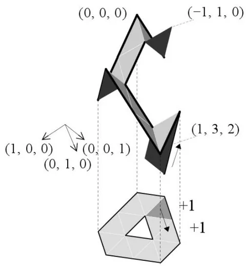
Proof. (Sketch of the proof) Let F be a regular flow in B. Let $T_B$ be a loop of F. Let $T_S$ be the slant trajectory on $T_B$ such that $\pi (T_S)=T_B$. Suppose that the pitch of $T_B$ is not zero. This would create a tear in the "cover" formed by the triangle of $T_S$. However, the starting point of the tear gives a singular base triangle.

d) Singular triangle detection by the pitch.

In the introduction, we examined the contour of a given loop from outside, and detected the presence of a singular triangle in the loop. Here we show that what we have calculated is nothing but the pitch of the loop.

Lemma 3.31. Let $I$ be an integer interval. Let

be a loop in $B$. Let $b[j]$, $b[k]\in T_B$ be adjacent triangles. Suppose that $b[j]$ and $b[k]$ are assigned the same normal edge (i.e., the edge shared by $b[j]$ abd $b[k]$ ). Then, $b[j-1]-b[j]-b[j+1]$ and $b[k-1]-b[k]-b[k+1]$ go in opposite directions.

Proof. Suppose that the two local flows go in the same direction. Then, the triangles in $T_B$ are connected in the following order:

In particular, two triangles $b[j-1]$ and $b[k+1]$ are separated by the closed chain

This means that the loop $T_B$ intersects with itself, which is a contradiction.

Proposition 3.32. A loop in B goes in the same direction on its contour. In particular, if you follow its contour along the loop stream, you will be going around the region occupied by the loop.

Proof. It follows from lemma 3.31 immediately.

Corollary 3.33. The pitch of a loop is obtained as follows:

Step 1 Divide the outer contour into a set of edges of triangles,

Step 2 Moving clockwise, assign either "+1" or "-1" to each edge of the contour. The rule of assignment is "change the sign if the direction of the edge changes".

The pitch of a loop is then obtained as the sum of all the "+1"s and "-1"s assigned.

Example 3.34. Let

(b)

(a)

Notes

(c) (d) Figure 6: Relation between flows. (a) Interaction "+" between loops. (b) Relation "<" between flows. (c) An upper bound $F_0$ of $\{F_1,F_2\}\subset F{W}_B$ (left) and the corresponding flows in S (right). (d) An upper bound $F_0$ of $\{F_1,F_2\}$ shown in a hybrid diagram be the loop in Figure 5 (a) below. This is the example considered in the introduction. Starting from the dark grey triangle, we obtain a $\{+1,-1\}$ -valued sequence of length 9:

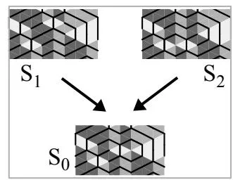
Summing them up, we obtain 3. On the other hand, let

be the lifted trajectory of $T_B$ (Figure 5 (a) above). Then,

Therefore,

Example 3.35. Let $T_B$ be the loop shown in Figure 5 (b) below. Starting from the dark grey triangle, we obtain a $\{+1,-1\}$ -valued sequence of length 12:

Summing them up, we obtain 0. On the other hand, the lifted trajectory of $T_B$ is a loop (Figure 5 (b) above). Therefore, $\mathrm{ptch}(T_B)=0$.

Example 3.36. Let $T_B$ be the loop shown in Figure 5 (c) below. Starting from the dark grey triangle, we obtain a $\{+1,-1\}$ -valued sequence of length 10:

Summing them up, we obtain 0. On the other hand, the lifted trajectory of $T_B$ is a loop (Figure 5 (b) above). Therefore, $ptch(T_B)=0$.

Ref In the last two examples, we were not able to detect the presence of singular triangles inside using the differential geometric approach. In the next section, we will show that a new approach can be used to detect both of the singular triangles.

IV. THE CATEGORY THEORETICAL APPROACH

In the previous approach, we examine the shape of the contour of a given loop. In the new approach, we will consider the interactions between a given loop and other loops in order to infer its internal structure. "Relations" between flows are then defined using the interactions between loops. The interactions between loops are determined only by their shape.

a) Relation between flows

Proteins are known to form protein-protein complexes as they perform their tasks. Also recognized recently is the importance of droplets of proteins (i.e., transient liquid-like assemblies of proteins) called "protein condensates" in protein-protein interactions $[8,9]$. In our mathematical toy model, proteins are represented as loops of triangles. Protein condensates then corresponds to a set of coexisting loops, i.e., (a region of) a flow of triangles. In order to model the interactions between proteins, we first define the interaction between loops as follows.

(a)

(b) (c) Figure 7: Suprema $\vee F_i$ and infima $\wedge F_i$ of flows in $B$. (a) Lower bounds and infima of $\{F_4,F_5\}$, upper bounds and suprema of $\{F_2,F_3\}$. (b) $\wedge$ -decomposition of $F_1^{\prime }$. (c) $\vee$ -decomposition of $F_2^{\prime }$. ( $F_i\to F_j$ denotes the relation $F_i⩽F_j$.)

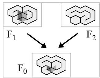
Definition 4.1 (Interaction between loops). Let

be loops of $B$ ( $n\in \mathbb{Z}$ ). We say that $l{p}_1,l{p}_2,\dots ,l{p}_n$ interact to form $l{p}_0$ if $l{p}_0$ contains all the triangles contained in $l{p}_1,l{p}_2,\dots ,l{p}_n$. Then, we denote the interactions using "+", i.e.,

We often write $\sum _{i=1,n}l{p}_i$ as an abbreviation for $l{p}_1+\dots +l{p}_n$.

Remark. Loops that are contained inside another loop are considered a part of the surrounding loop.

Remark. Since there may be multiple loops with the same contour, loop $\sum _{i=1,n}l{p}_i$ is not uniquely determined. However, the contour of $\sum _{i=1,n}l{p}_i$ is uniquely determined.

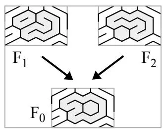
Example 4.2. In Figure 6 (a), two loops $l{p}_1$ and $l{p}_2$ interact to form a loop. Note that $l{p}_1+l{p}_2$ contains a loop of length 6 inside. In this case, $l{p}_1+l{p}_2$ is uniquely determined.

In order to characterize a protein by its interaction with other proteins, it is necessary to take into account a droplet of proteins that contains the protein. In our model, we need to consider flows that contain the given loop. The "category" of flows is defined as follows.

Definition 4.3 (The set $F{W}_B$ of all flows in B). We de note by $F{W}_B$ the set of all flows in B. $F{W}_B$ is the "object" we consider in the new approach. Let $F\in F{W}_B$. We denote by $Lp(F)$ the set of all loops of F. In the following, we will identify F with $Lp(F)$ since we do not consider interactions between loops (i.e., closed trajectories) and open trajectories. Let $F_1,F_2\in F{W}_B$. We write

if $Lp(F_1)=Lp(F_2)$. " $\mathrm{\Xi }$ " gives an equivalence relation on $F{W}_B$. We denoted by Z the flow with no loop. Z is unique up to " $\mathrm{\Xi }$ ".

Using the interaction "+" between loops, we define a relation on $F{W}_B$.

Definition 4.4 (Relation " $⩽$ " on $F{W}_B$ ). Let $F_1,F_2\in F{W}_B$. We define a binary relation " $⩽$ " on $F{W}_B$ by

if and only if, for any $l{p}^{\prime }\in Lp(F_2)$, there is a set

Notes

$(n\in \mathbb{Z})$ such that

We write if $F_1⩽F_2$ and $F_1\ne F_2$. By the conventions of Category theory, we often write $F_1\to F_2$ instead of $F_1⩽F_2$ (especially in the figures).

Example 4.5. In Figure 6 (b), since $l{p}_0=l{p}_1+l{p}_2$.

b) Covering flow of regular flows.

"Suprema" (i.e., least upper bounds) and "infima" (i.e., greatest lower bounds) are defined as follows.

Definition 4.6 (Upper bound and lower bound). Let $C\subset F{W}_B$. Let $M\in F{W}_B$. $M$ is called an upper bound of $C$ if for all $F\in C$. $M$ is called a lower bound of $C$ if for all $F\in C$. An upper (resp. lower) bound $M$ is called regular if $M$ is a regular flow.

Remark. An upper bound (resp. lower bound) $M$ of $C$ is not contained in $C$.

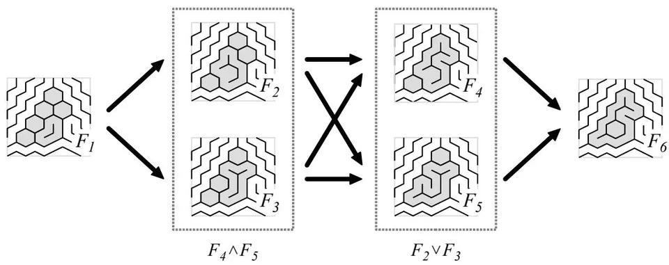
Example 4.7. In figure 6 (c) left, $F_0$ is an upper bound of $\{F_1,F_2\}$. In figure 6 (c) right, the flow $S_0$ (resp. $S_1,S_2$ ) in S corresponds to the flow $F_0$ (resp. $F_1,F_2$ ) in B. As you can see, $S_0$ is obtained by putting a cube on $S_2$. $S_1$ is then obtained by putting one more cube on $S_0$. In this way, we can compute fusion and fission of loops immediately. In Figure 6 (d), the added cubes are drawn to show the process of computation.

Remark. In the following, "Figure 6 (d)"-style figures will be often used instead of "Figure 6 (c)"-style figures when describing the relation between flows.

Definition 4.8 (Supremum $\vee$ ). Let $C\subset F{W}_B$. Let $M\in F{W}_B$ be an upper bound of $C$. $M$ is called a supremum of $C$ if $M⩽M^{\prime }$ for any upper bound of $C$. We denote by $\vee C$ the set of all suprema of $C$. If $C=\{F_1,F_2,\dots ,F_n\}$, we often write $F_1\vee F_2\vee \cdots \vee F_n$ or ${\nu }_{i=1,n}{F}_i$ instead of $\vee \{F_1,F_2,\dots ,F_n\}$. $C$ often has more than one supremum.

Definition 4.9 (Infimum $\mathrm{\Lambda }$ ). Let $C\subset F{W}_B$. Let $N\in F{W}_B$ be a lower bound of $C$. $N$ is called an infimum of $C$ if $\dot{N}⩽N$ for any lower bound $\dot{N}$ of $C$. We denote by $\wedge C$ the set of all infima of $C$. If $C=\{F_1,F_2,\dots ,F_n\}$, we often write $F_1\wedge F_2\wedge \cdots \wedge F_n$ or ${\wedge }_{i=1,n}{F}_i$ instead of $\wedge \{F_1,F_2,\dots ,F_n\}$. $C$ often has more than one infimum.

Example 4.10. In figure 7 (a), $F_4\wedge F_5=\{F_2,F_3\}$ and $F_2\vee F_3=\{F_4,F_5\}$. Since $F_2\setminus F_1,F_1\in /F_4\wedge F_5$. Since $F_6⩽̸F_4$, $F_6\notin F_2\wedge F_3$.

Example 4.11. ( $\wedge$ -decomposition) In Figure 7 (b), all upper bounds of $F_1^{{}^{\prime }}$ are shown in the rectangle. Using three of them, we have $\{F_1^{\prime }\}=F_3^{{}^{\prime }}\wedge F_4^{{}^{\prime }}\wedge F_5^{{}^{\prime }}$. (Let $F_a$ and $F_b$ be flows with one loop. Then, $F_a\vee F_b=\{Z\}$. For example, $F_2^{{}^{\prime }}\vee F_3^{{}^{\prime }}=\{Z\}$.)

Example 4.12. (V-decomposition) In Figure 6(c), all lower bounds of ${\overrightarrow{F}}_2$ are shown in the rectangle. Using three of them, we have $\{F_2^{\prime }\}=F_1^{\prime }\vee F_7^{\prime }\vee F_8^{\prime }$.

In order to characterize the contour of a given loop $lp$, we consider the set of all lower bounds of a flow $F$ such that $Lp(F)=\{lp\}$. (Note that $F$ has no upper bound other than $Z$.)

Notes

Definition 4.13 (Covering flow of a flow in B). Let $F\in F{W}_B$. We denote by $Cv(F)$ the set of all regular lower bounds of F, i.e.,

Flows of $Cv(F)$ are called covering flows of F. The minimum elements of $Cv(F)$ are called generators of $Cv(F)$. The dimension of $Cv(F)$ is defined as the number of its generators.

Lemma 4.14 (V-decomposition). Let $F\in F{W}_B$ be a regular flow. Then, $\{F\}=\vee Cv(F)$.

Proof. It follows immediately from the definition.

Remark. If F is a singular flow, then $Cv(F)=\mathrm{\varnothing }$. We will consider covering flows of a singular flow in section 4.4 below.

By considering the set of all covering flows, we can distinguish loops with similar contours, as the following examples show.

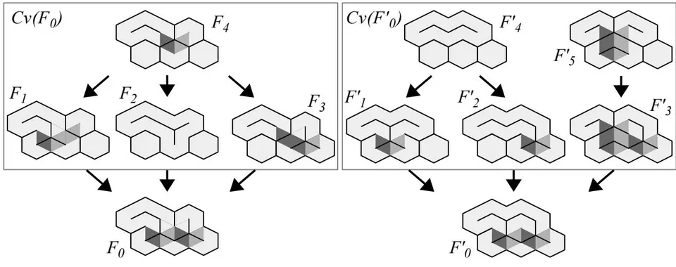
Example 4.15. In Figure 8 (a), $F_0$ is a flow such that $Lp(F_0)$ consists of one loop. $Cv(F_1)$ consists of four flows. $Cv(F_1)$ has one generator $F_4$. The dimension of $Cv(F_1)$ is one. Moreover,

(a) (b)

Notes

(c) (d) Figure 8: Covering flows. (a) and (b) Covering flows of flows in B. (c) and (d) Covering flows of regions of B.

Example 4.16. In Figure 8 (b), $F_0^{\prime }$ is a flow such that $Lp(F_0^{\prime })$ consisting of one loop. $Cv(F_1)$ consists of five flows. $Cv(F_1)$ has two generators $F_4^{\prime }$ and $F_5^{\prime }$. The dimension of $Cv(F_1^{\prime })$ is two. Moreover,

c) Closure of $F{W}_B$ with respect to "V".

Let $C\subset F{W}_B$. Then, $\vee C$ often contains no flows other than $Z$, i.e., $\vee C=\{Z\}$. For example, let $C$ be the set of all flows such that their loops sweep a given region collectively. Then, $\vee C=\{Z\}$ if there is no loop with the contour of the region. However, since we want to treat both protein complexes and proteins seamlessly, we treat the "contour made up of multiple loop contours" in the same way as the "contour of a single loop".

Definition 4.17 (Covering flow of a region of B). Let R be a region of B. We denote by $Cv(R)$ the set of all regular flows such that the region swept by their loops matches the region R. Flows of $Cv(R)$ are called covering flows of R. The minimum elements of $Cv(R)$ are called generators of $Cv(R)$. The dimension of $Cv(R)$ is defined as the number of its generators.

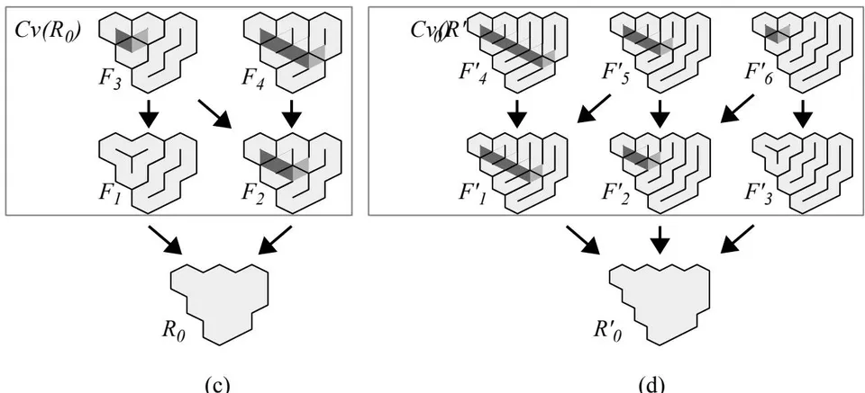
Example 4.18. In Figure 8 (c), $Cv(R_0)$ consists of four flows. Since it has two generators, its dimension is two. Since there is no loop whose contour matches the contour of $R_0$, $\vee Cv(R_0)=\{Z\}$.

Example 4.19. In Figure 8 (d), $Cv(R_0^{\prime })$ consists of six flows. Since it has three generators, its dimension is three. Since there is no loop whose contour matches the contour of $R_1$, $\vee Cv(R_0^{\prime })=\{Z\}$.

Now let us extend $F{W}_B$ to include "virtual" loops with contours made up of multiple contours of loops.

First, we identify the set $F{W}_B$ of flows in B with the set of $\{0,1\}$ -valued functions on $F{W}_B$.

Definition 4.20 (Hom-Sets). Let $F_1,F_2\in F{W}_B$. In the language of Categories, the set of all the possible relations between $F_1$ and $F_2$ is denoted by $\mathrm{Hom}(F_1,F_2)$, i.e.,

Notes where 1 denotes a set with one element and 0 denotes a set with no element. We define a binary relation on $\{0,1\}$ by

We write $a⩽b$ if or $a=b$. We define multiplication "." on $\{0,1\}$ by

We often write ${}^{ab}$ instead of $a\cdot b$ when there is no risk of confusion.

Remark. Let $F,X\in F{W}_B$ Roughly speaking, X is a "refinement" of F if $Hom(X,F)=1$. X is a "component" of F if $Hom(F,X)=1$.

Remark. $\{0,1\}$ is a category equipped with two objects $\{0,1\}$ and three relations 0<1,0=0, and 1=1.

Hom-sets provide two types of $\{0,1\}$ -valued functions on $F{W}_B$: one is order-preserving function and the other is order-reversing function.

Definition 4.21 (Hom functions on $F{W}_B$ ). Let $F,X,Y\in F{W}_B$.

(1) Order-preserving function $k(F)$ on $F{W}_B$ is defined by

Note that $X⩽Y$ implies $k(F)(X)⩽k(F)(Y)$.

Note that $X⩽Y$ implies $h(F)(X)⩾h(F)(Y)$.

Definition 4.22 ( $F{W}_B^{\vee }$ and $F{W}_B^{\wedge }$ ). (1) We denote by $F{W}_B^{\vee }$ the set of all order-preserving functions from $F{W}_B$ to $\{0,1\}$. Let $h_0,h_1\in F{W}_B^{\vee }$. We then define a binary relation " $⩽$ " on $F{W}_B^{\vee }$ by

for all $X\in F{W}_B$.

for all $X\in F{W}_B$

Note that k is a function defined by

$h$ is a function defined by

Ref

We can then identify $F{W}_B$ as a subcategory of $F{W}_B^{\vee }$ (resp. $F{W}_B^{\wedge }$ ) by k (resp. h). Recall that $F\equiv G$ if and only if $Lp(F)=Lp(G)$.

Proposition 4.23. (1) k is a one-to-one function (up to "≡"). (2) h is a one-to-one function (up to "≡").

Proof. It follows from the the Yoneda lemma ([6]).

Functions in $F{W}_B^{\vee }$ (or $F{W}_B^{\wedge }$ ) are called "representable" if they correspond to "actual" flows in B. That is,

Definition 4.24 (Representable function on $F{W}_B$ ). (1) Let $c\in F{W}_B^{\vee }$. $c$ is called representable if there is a flow $F\in F{W}_B$ such that

$F$ is called a representation of $c$.

(2) Let $c\in F{W}_B^{\wedge }$. $c$ is called representable if there is a flow $F\in F{W}_B$ such that

$F$ is called a representation of $c$.

Example 4.25. In the case of Figure 8 (c), define $h_0\in F{W}_B^{\wedge }$ by

Then,

Since $h(F_1)(F_2)=0$, $h_0\ne h(F_1)$. Since $h(F_2)(F_1)=0$, $h_0\ne h(F_2)$. Since $h(Z)(X)=1$ for all $X\in F{W}_B$, $h_0\ne h(Z)$. Moreover, $h_0$ is not representable. Thus, we can regard $h_0$ as the "virtual" loop whose contour matches the contour of $R_0$.

Ref

Example 4.26. In the case of Figure 8 (d), define $h_1\in F{W}_B^{\wedge }$ by

Then,

Since $h(F_1^{\prime })(F_2^{\prime })=0$, $h_1\ne h(F_1^{\prime })$. Since $h(F_2^{\prime })(F_1^{\prime })=0$, $h_1\ne h(F_2^{\prime })$. Since $h(F_3^{\prime })(F_1^{\prime })=0$, $h_1\ne h(F_3^{\prime })$. Since $h(Z)(X)=1$ for all $X\in F{W}_B$, $h_1\ne h(Z)$. Moreover, $h_1$ is not representable. Thus, we can regard $h_1$ as the "virtual" loop whose contour matches the contour of $R_1$.

Example 4.27 (Heyting algebra [10]). Let A be the flow obtained by dividing B into a hexagonal lattice. That is, $L_p(A)$ consists of an infinite number of hexagonal shaped loops of length 6. Let $X,Y\in F{W}_B$. We define the negation $\mathrm{\neg }X$ of X and an exponential $Y^X$ by

In general, neither is representable.

d) Branched covering of singular flows.

Here we define "extended covering flows" of a singular flow. For simplicity, we will only consider the flows of $F{W}_B$, not the flows of $F{W}_B^{\vee }$ or $F{W}_B^{\wedge }$

Definition 4.28 (Regular loop). A loop is called regular if it contains no singular triangles inside.

Remark. We can embed a regular loop in a regular flow.

Definition 4.29 (Relation " ${⩽}_X$ " on $F{W}_B$ ). Let $F_1,F_2\in F{W}_B$. We define a binary relation " ${⩽}_X$ " on $F{W}_B$ by

Notes

if and only if, for any regular loop $l{p}^{\prime }\in Lp(F_2)$ there is a set

$(n\in \mathbb{Z})$ such that

We write if $F_1{⩽}_X{F}_2$ and $F_1\ne F_2$.

We then extend the relation " ${⩽}_X$ " on the set $P(F{W}_B)$ of all subsets of $F{W}_B$.

Definition 4.30 (Relation " ${⩽}_X$ " on $P(F{W}_B)$ ). Let $P_1,P_2\in P(FL{W}_B)$. We define a binary relation " ${⩽}_X$ " on $P(F{W}_B)$ by

if and only if, for any regular loop $l{p}^{\prime }\in Lp(F^{\prime })$ of $F^{\prime }\in P_2$, there are $F\in P_1$ and

$(n\in \mathbb{Z})$ such that

We write if $P_1{⩽}_X{P}_2$ and $P_1\ne P_2$.

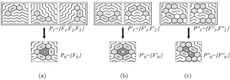
Example 4.31. In Figure 9, , , and .

Aligned

Not aligned

(a)

(c) Enclosed

Not enclosed

(b) Loop neighborhood

Singular flow

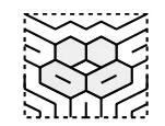
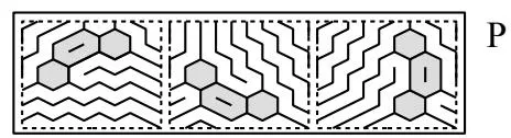
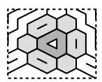
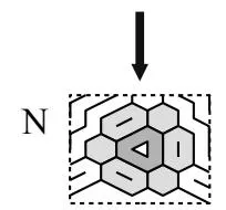
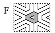
Figure 10: Multiplicity of signular flows. (a) Aligned flow. (b) Enclosing neighborhood of a loop. (c) Computation of the multiplicity of a loop

Definition 4.32 (Branched lower bound). Let $C\subset P(F{W}_B)$. Let $P\in P(F{W}_B)$. $P$ is called a branched lower bound of $C$ if

Flows contained in a branched lower bound P are called the sheets of P. A branched lower bound P is called regular if P consists only of regular flows.

Example 4.33. In figure 9, $P_1$ (resp. $P_1^{{}^{\prime }}$, $P_1^{{}^{″}}$ ) is a branched lower bound of one-element set $P_0$ (resp. $P_0^{{}^{\prime }}$, $P_0^{{}^{″}}$ ). $P_1$ contains three sheets. $P_1^{{}^{\prime }}$ and $P_1^{{}^{″}}$ contains two sheets.

Notes

Definition 4.34 (Branched covering of a flow). Let $F\in F{W}_B$. We denote by $BCv(F)$ the set of all regular branched lower bounds of $\{F\}$, i.e.,

Elements of $BCv(F)$ are called branched covering of F. Roughly speaking, the sheets of a branched covering collectively cover F. The multiplicity $m(P)$ of a branched covering P is defined as the number of sheets of P.

Example 4.35. In Figure 9, $P_1$ (resp. $P_1^{{}^{\prime }}$, $P_1^{{}^{″}}$ ) is a branched covering of $F_0$ (resp. $F_0^{{}^{\prime }}$, $F_0^{{}^{″}}$ ). Then, $m(P_1)=3$, $m(P_1^{\prime })=2$, and $m(P_1^{\prime \prime })=2$.

e) Multiplicity of loops.

Let $F\in F{W}_B$. Let $lp\in Lp(F)$. To capture the "turbulence" of the flow $F$ around the loop $lp$, we consider a set of loops surrounding $lp$.

Definition 4.36 (Aligned flow). Let $F\in F{W}_B$. $F$ is called aligned if, for any pair $l{p}_1$, $l{p}_2\in Lp(F)$, the vertices of the contour of $l{p}_1$ are not contained in the interior of the edges of the contour of $l{p}_2$ (Figure 10 (a)).

Definition 4.37 (Enclosing neighborhood of a flow). Let $N,F\in F{W}_B$. $N$ is called an enclosing neighborhood of $F$ if $Lp(F)\subset Lp(N)$ and the contour of the region swept by $Lp(N)$ dose not contain the vertices of the contour of $Lp(F)$.

Example 4.38. In Figure 10 (b), F consists of one flow (colored dark grey). In Figure 10 (b) left, the dark grey loop is enclosed by a set of six loops. On the other hand, in Figure 10 (b) right, a part of the grey loop is exposed outside.

Remark. $N{⩽}_{X}F$ if N is an enclosing neighborhood of F.

Definition 4.39 (Loop neighborhood of a loop). Let $F\in F{W}_B$. Let $N$ be an enclosing neighborhood of $F$. $N$ is called a loop neighborhood of $F$ if $N$ is aligned.

Definition 4.40 (Multiplicity of a flow). Let $F\in F{W}_B$. The multiplicity $\text{mul}(F)$ of flow $F$ is defined by

If $Lp(F)=\{lp\}$, $mul(F)$ is called the multiplicity of loop $lp$ and denoted by $mul(lp)$.

Remark. The multiplicity of an affine flow is one.

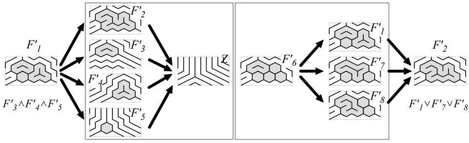
Figure 10 (c) shows the computation process of the singular loop considered in the introduction (Figure 1). Suppose that we are given a flow F consisting of the singular loop (lower right).

First, find a loop neighborhood N of the flow (lower left). In this case, N contains three regular loops of length six, three regular loops of length 10, and the singular loop.

Next, find a branched covering P of N (upper left). In this case, P has three sheets. Because of the overlap of the lifted trajectories in S, two of the three regular loops of length 10 cannot be embedded in one sheet at the same time. That is,

With a little consideration, we can see that N give the minimum multiplicity, i.e.,

Remark. Let $N,N^{\prime }$ be two loop neighborhoods of the same flow $F$. The author dose not know whether

or not.

f) Singular triangle detection by the multiplicity

Recall that the aim of this paper is to detect the presence of singular triangles inside by examining the outer contour of a given loop. Since we can compute the multiplicity of a loop from the outside, we can use the multiplicity of the loop for that porpose.

Proposition 4.41. Let $F\in F{W}_B$.

(1) If , then $F$ is a singular flow.

(2) If $mul(F)=1$, then $ptch(lp)=0$ for all $lp\in Lp(F)$.

Proof. It follows immediately from the definition.

Corollary 4.42. Let lp be a loop of B. If , then there are singular triangles inside lp.

Example 4.43. In Figure 9 (a), the dark grey loop lp of $F_0$ contains singular loops inside since . Note that $F_0$ is a loop neighborhood of a flow consisting only of lp.

Example 4.44. In Figure 9 (b), the dark grey loop $l{p}^{\prime }$ of $F_0^{\prime }$ contains singular loops inside since . Note that $F_0^{\prime }$ is a loop neighborhood of a flow consisting only of $l{p}^{\prime }$.

Example 4.45. In Figure 9 (c), the dark grey loop $l{p}^{″}$ of $F_0^{″}$ contains singular loops inside since . Note that $F_0^{″}$ is a loop neighborhood of a flow consisting only of $l{p}^{″}$.

Recall that in the last two examples, the differential geometry approach failed to detect the presence of singular triangles inside (Example 3.35 and 3.36).

V. CONCLUSION

Using a simple mathematical model, we have presented two approaches to inferring the internal structure of proteins from the outside. One is the differential geometric approach proposed in [1]. The other is a new category theoretical approach proposed in this paper.

In the former approach, we calculate the pitch of a given loop. In the latter approach, we compute the multiplicity of a neighborhood of a given loop. We then showed that the new approach can detect more singular triangles inside than the previous approach.

VI. DISCUSSION

This research is intended to be applied to the structural study of proteins. First, we represented proteins as a loop of triangles (i.e., 2-simplices). Second, we proposed a new method to infer the internal structure of a protein (i.e., a loop) from the turbulence of a droplet (i.e., a loop neighborhood) surrounding the protein. Third, as an example, we considered the detection of singularities (i.e., singular triangles) in a protein.

In relation to these three points, three issues come to mind for discussion: first, how to approximate the shape of a protein using the loops of n-simplices; second, how to measure the turbulence (multiplicity) of a droplet of biomolecules surrounding a protein; and third, why we considered singular triangle detection. Let us discuss these issues in turn.

(1) Due to strong constraints on the geometry of loops of n-simplices, it is not straightforward to approximate the folded structure of proteins using a loop of n-simplices. However, it is this simplification that allowed us to obtain a simple mathematical model of the relation between the internal structure and the external shape of proteins. The author hopes that this research will serve as a stepping stone to obtain better mathematical models of proteins in the future, which can handle the internal structure and the external shape simultaneously.

(2) In recent years, droplets of biomolecules have been witnessed everywhere in cells. In particular, the idea that their functions emerge from the collective behaviors of the molecules has become the central concept in condensate biology ([9]). However, since droplets are often formed transiently, it is difficult to measure their movement. Nevertheless, the author believes that even ridiculous needs can lead to the development of novel measurement techniques for droplets.

Finally, the author would like to mention some future research topics.

(3) Flows in higher dimensions. When applied to protein structure analysis, we need to consider loops of tetrahedra. There seems to be a large gap in difficulty between the study of flows of triangles and the study of flows of n-simplices . However, because of the simplicity of the model, the author believes that we can jump over the gap and think about flows in higher dimensions. Even with this simple model, the gap may produce interesting results in higher dimensions.

Conflict of Interest

The author declares that there is no conflict of interest regarding the publication of this paper.