Type Ii Half Logisitic Exponentiated Lomax Distribution

Bukoye Abdulwasiu; Bada Olatunbosn; Muritala Abdulkabir; Ajadi, A.Akeem

I. INTRODUCTION

Lomax distribution can also be called Pareto Type II distribution and its application can be found in many fields like actuarial science, economics, and so on Al-Zahrani and Al-Sobhi (2013). The distribution was defined by Lomax (1954) and it is a heavy-tailed distribution. It has also been considered to be useful in reliability and life testing problems in engineering and in survival analysis as an alternative distribution Kilany (2016), Hassan and Al-Ghamdi (2009).

Modified and extended versions of the Lomax distribution have been studied; examples include the weighted Lomax distribution by Kilany (2016), exponential Lomax distribution by El-Bassiouny et al (2015), exponentiated Lomax distribution by Salem (2014), gamma Lomax distribution Cordeiro et al (2015), transmuted Lomax distribution by Ashour and Eltehiwy (2013), Poisson Lomax distribution by Al-Zahrani and Sagor (2014), McDonald Lomax distribution by Lemonte and Cordeiro (2013), Weibull Lomax distribution by Tahir et al (2015), and power Lomax distribution [12]. Besides, estimation of the parameters of Lomax distribution under general progressive censoring has also been considered by Al-Zahrani and Al-Sobhi by Al-Zahrani and Al-Sobhi (2013).

The half logistic distribution is a member of the family of logistic distributions which is introduced by (Balakrishnan, 1985) which has the following cumulative distribution function (CDF)

Hassan et al. (2017) use the half logistic generator instead of the gamma generator to obtain type II half logistic family, which is denoted by TIIHL-G. Then the CDF and pdf of TIIHL-G is defined as follows

Notes

Where $\lambda$ is the shape parameter and $g(x;\lambda)$ , and $G(x;\lambda)$ is the baseline distribution, respectively.

However, the TIIHLEE has tractable properties, especially for simulation, since its quantile function takes a simple form.

Where u is a uniform distribution on the interval $(0,1)$ and $G^{1}$ (.) is the inverse function of $G(\cdot)$

Our aim in this work is to study a modified statistical distribution that will be suitable to fit positively skewed and unimodal data and to check the flexibility of the existing and proposed distribution.

II. TYPE II HALF LOGISTIC EXPONENTIATED LOMAX DISTRIBUTION

The cumulative density function (CDF) and probability density function (pdf) of exponentiated Lomax distribution (EE) are defined as follows:

Substituting 6 and 7 in 4 and 3 then we define probability density function (pdf) and cumulative density function (CDF) Type II Half Logistic Exponentiated Lomax Distribution (TIIHLEL) as follows:

Henceforth, a random variable with probability density function (pdf) is denoted by $X \sim TIIHLEL(\alpha, \beta, \lambda, \theta)$

Notes

a) Hazard Function of TIIHLEL

b) Survival Function of TIIHLEL

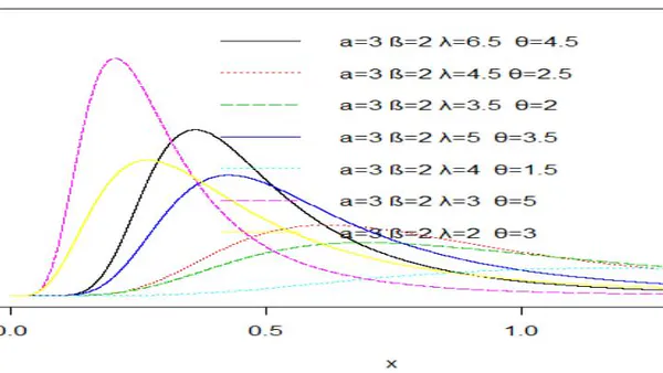
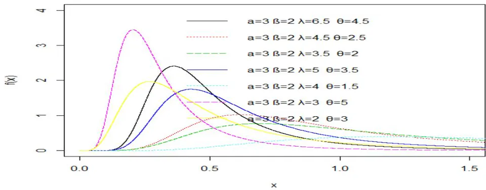
Plots of the density function (8) can be represented through Fig. 1. As it seems from Fig. 1 that the pdf of TIIHLEL can take different shapes according to different values of $\theta$ and $\lambda$ . It can be symmetric, right-skewed, unimodal

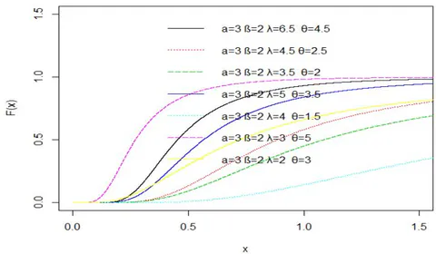
Figure 1: Plot of the Density function of TIIHLEL

Plots of cumulative distribution function (9) for the TIIHLEL distribution are displayed in Fig. 2. The CDF graph tends to move at a constant value from 0 to 1 on the x-axis before projecting to one on the y-axis

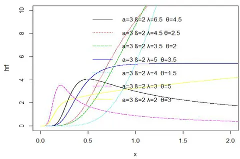
Figure 2: Plot of the Distribution function (CDF) of TIIHLEL

Plots of hazard function (10) for the TIIHLEL distribution are displayed in Fig. 3 It was examined from Fig. 3 show that the shape of the h(x) of the TIIHLEL shows the hazard functions can be constant, increasing or decreases, depending on the shape and scale parameters.

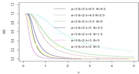
Figure 3: Plot of the Hazard function of TIIHLEL

Plots of survival function (11) for the TIIHLEL distribution are displayed in Fig. 4. It was deduced from Fig. 4 that the shape parameters have a strong effect on the survival plot. A decrease in the shape parameter tends to reduce the movement of the line on the y-axis, and no plot is exceeding the benchmark of 1

Figure 4: Plot of the Survival function of TIIHLEL

c) Some Special case of TIIHLEL

When $\alpha=1$ , the TIIHLEL model reduces to Type II half Logistic Lomax (TIIHLL) model with $\lambda$ and $\theta$ as shape parameters and $\beta$ as a scale parameter.

Notes

When $\beta=1$ , the TIIHLEL model reduces to Type II half Logistic Exponentiated Pareto (TIIHLEP) model with $\lambda$ , $\theta$ , and $\alpha$ as shape parameters.

When $\lambda=1$ , the TIIHLEL model reduces to Half Logistic Exponentiated Lomax (HLEL) model with $\alpha$ and $\theta$ are shape parameters $\lambda$ is scale parameter.

When $\alpha=\beta=1$ , the TIIHLEL model reduces to Type II Half Logistic Pareto (TIIHLP) model with $\lambda$ and $\theta$ as shape parameters.

When $\alpha=\lambda=1$ , the TIIHLEL model reduces to Half Logistic Lomax (HLL) model with $\lambda$ and $\theta$ and $\alpha$ are shape parameters.

When $\alpha=\lambda=\beta=1$ , the TIIHLEL model reduces to Half Logistic Pareto (HLP) model with $\theta$ as a scale parameter.

Table 1: Summary of Sub-Models from the TIHLEL distribution

Distribution	$\alpha$	$\beta$	$\lambda$	$\theta$
TIIHLL	1	$\beta$	$\lambda$	$\theta$
TIIHLEP	$\alpha$	1	$\lambda$	$\theta$
HLEL	$\alpha$	$\beta$	1	$\theta$
TIIHLP	1	1	$\lambda$	$\theta$
HLL	1	$\beta$	1	$\theta$
TIIHLEL	1	1	1	$\theta$

Table 1 depict some existing model obtained when some parameters of the proposed distribution are relaxed.

III. MATHEMATICAL PROPERTIES FOR TIIHLEL

a) Infinite Linear Combination

Let $v = \lambda a$

Notes

Let

b) Moment of Proposed TIIHLEL Distribution

It is imperative to derive the moments when a new distribution is proposed. They play a significant role in statistical analysis, particularly in applications. Moments are used in computing measures of central tendency, dispersion, and shapes, among others.

Suppose the $r^{th}$ moment for the TIIIHL-G family is derived.

Let

Notes

Beta function is given

Therefore $y=\theta_{k}+\theta_{i}+\theta-r$

Comparing 3.79 and 3.80 we have

The mean of the proposed TIIHLEL distribution is gotten by making $\mu^{r}$ moment equal to one (—r=1)

When $r = 2$

When $r = 3$

When $r=4$

The variance of TIIHLEL is obtained.

Substituting equation 17 and 18 into 21 to obtain the variance of TIIHLEL

Standard Deviation of TIIHLEL

Coefficient of Variation of TIIHLE (Theta)

c) Moment Generating Function of TIIHLEE Distribution

A random variable x with pdf f(x) is defined as a

d) Incomplete Moment

The incomplete moment plays an important role in computing the mean deviation, median deviation.

The $r^{th}$ incomplete moment of the TIIHLEL is given by

Where B(..) is the incomplete beta function and r=1,2,3.....

The variation in a population can be measured to some degree by the totality of deviations from the mean and the median. If the random variable X follows the TIIHLEL distribution, then the mean and the median deviations are given as

Notes

Where $\int_0^\mu xg(x)dx$ is simplified using the first incomplete moment

a) Renyi Entropy

Entropy plays a vital role in science, engineering, and probability theory, and has been used in various situations as a measure of variation or uncertainty of a random variable (Renyi, 1961). The Renyi entropy of TIIHLEL is given as

b) Quantile and Median

Simulation methods utilize quantile function to produce simulated random variables for classical and new continuous distributions.

The inverse of the CDF in (6) yields the quantile function of the

When p = 0.25, 0.5 and 0.75 we obtain the first quantile, median and third quartile of TIIHLEL distribution In particular $Q(0.5) = F^{-1}(u)$ is the median of the probability distribution given as

The median of TIIHLEL Distribution can be obtained by equating equation 28 to 0.5

c) Order of Statistics

Let $Y_1, Y_2, \ldots, Y_n$ be independently and identically distributed (i.i.d) random variable with their corresponding cumulative function (cdf) $F(x)$ . Let $X_{(1)}$ be the smallest (first-order statistic) of the $Y_1, Y_2, \ldots, Y_n$ , $X_{(2)}$ is the second-order statistics greater than $X_{(1)}$ , and $X_{(n)}$ is the largest order statistics. Hence, $X_{(1)} < X_{(2)} \ldots < X_{(n)}$ is the order statistics corresponding to random variable $Y_1, Y_2, \ldots, Y_n$ (see Kapur and Sexena (1960)).

Notes

The density $f_{n:i}(x)$ of the ith order statistics, for $i = 1, \ldots, n$ , from independent identical distribution random variable $Y_{1} \ldots Y_{n}$ is given by

i. Order Statistic of TIIHLEL

$B(.,.)$ is the beta function. The pdf of the $\mathbf{r}^{\mathrm{th}}$ order statistic for TIIHLEL distribution is derived by substituting (6) and (7) in (30) as follows.

Applying the binomial expansion (12) in (31), then we have

Again, using the binomial expansion (12) in the previous equation, then the pdf of the $r^{th}$ order statistic for TIIHLEE distribution is obtained as follows.

The distribution of the smallest and largest order statistics are obtained by putting r=1 and r=n in (32) respectively as follows.

However

ii. Skewness and kurtosis of the TIIHLEL distribution

Skewness is used to measure the asymmetry, and kurtosis is used to measure the peakedness of probabilistic models. Both measures are the descriptive measures of the shape of the probability distribution.

The skewness and Kurtosis of TIIHLEE are given as follows:

Notes

And

a) Maximum Likelihood Estimator (MLE) for TIIHLEL

Let $x_{1}; x_{2}; \ldots, x_{n}$ be a random sample of size n from the TIIHL family of distributions $(\alpha; \beta; \lambda, \theta)$ . The log-likelihood function for the vector of parameters $L = (\alpha; \beta; \lambda, \theta)^{T}$ can be expressed as

The log-likelihood function is expressed as and let $w = (1 + \beta x)^{-\theta}$

Taking the first partial derivatives of $\ell(x;\alpha,\beta,\lambda,\theta)$ of (36) with respect to $\alpha,\beta,$ and $\lambda$ and letting them equal zero, we obtain a nonlinear system of equations.

Notes

The above-derived equations are in the complex form; therefore, the exact solution of ML estimator for unknown parameters is not possible. So it is convenient to use nonlinear Newton Raphson algorithm for exact numerically solution to maximize the above likelihood function.

However, the above equation cannot be solved analytically, and statistical software can be used to solve them numerically using iterative methods.

Solving the nonlinear system of the equation of $\frac{\partial l}{\delta\alpha}=0\frac{\partial l}{\delta\beta}=0\frac{\partial l}{\delta\lambda}=0$ , and $\frac{\partial l}{\delta\theta}=0$ we then obtain the Maximum likelihood estimate $\alpha$ , $\beta$ , $\lambda$ , and $\theta$ respectively. Information matrix of 4x4 will be obtained through

The solution to the above equation inverse dispersion matrix yields the asymptotic variance and covariance of the maximum likelihood estimators $\hat{\alpha},\hat{\beta},\hat{\lambda}$ and $\theta$

b) Confidence Interval for the Parameters

The approximate confidence intervals for $100(\alpha - 1)\%$ for $\alpha$ , $\beta$ and $\lambda$ is given respectively by

Where the $Z_{\frac{\alpha}{2}}$ is the $\alpha^{th}$ percentiles of the standard normal distribution.

VI. SIMULATION STUDY FOR TIIHLEL DISTRIBUTION

A simulation study was carried out to check MLE of TIIHLEL for different sample size n=10 and 100 in order to obtain Mean, Median, Standard Deviation, Skewness, and Kurtosis of the parameters. The quantile function of TIIHLEL used for simulation studies is given in (28) with $\alpha$ , $\theta$ , and $\lambda$ as shape parameters while $\beta$ is a scale parameter.

Table 2: The Mean, Median and Standard of TIIHLEL Distribution for

\beta = 2

, 4 and 6 for

n = 10

α	λ	θ	β=2			β=4			β=6
α	λ	θ	Mean	Median	SD(σ)	Mean	Median	SD(σ)	Mean	Median	SD(σ)
0.5	0.5	0.5	0.4568	0.1146	1.1677	-0.0612	-0.0378	0.0769	-0.1373	-0.0853	0.1412
		0.8	72.4466	-0.000	321.5256	36.1165	-0.0098	160.6742	24.006	-0.0201	107.0571
		2.5	3.6512	-0.0056	15.774	1.7188	-0.0401	7.7977	-0.1627	-0.0956	0.1772
		5	0.0246	-0.0332	0.3320	-0.1373	-0.0853	0.1412	-0.1341	-0.0942	0.1322
	0.8	0.5	-0.1341	-0.0942	0.1322	-0.1088	-0.0976	0.0949	-0.2155	-0.1901	0.1574
		0.8	73.5713	-0.0064	325.9628	36.6245	-0.04936	162.9039	24.3089	-0.0681	108.551
		2.5	187.2195	0.1497	829.0332	1.6962	-0.1042	7.9176	1.0233	-0.1337	5.2270
		5	-0.0145	-0.0783	0.3475	-0.1684	-0.1486	0.1606	-0.2197	-0.1763	0.1596
	2.5	0.5	-0.2416	-0.2967	0.1691	-0.4400	-0.5243	0.1643	-0.4400	-0.5243	0.1643
		0.8	0.6782	0.2158	1.8055	-0.1262	-0.1435	0.1140	-0.1810	-0.3735	0.5405
		2.5	0.0746	-0.0577	0.5156	-0.2693	-0.3163	0.0931	-0.3823	-0.4944	0.1715
		5	-0.2266	-0.2808	0.0830	-0.2680	-0.3727	0.2282	-0.4827	-0.5773	0.1776
	5	0.5	-0.4969	-0.5906	0.1889	-0.3401	-0.3798	0.0684	-0.5510	-0.6165	0.1233
		0.8	0.7013	0.2536	1.9227	-0.0302	-0.2838	0.9234	-0.2741	-0.4728	0.5955
		2.5	0.0424	-0.0785	0.5637	-0.3597	-0.4515	0.2536	-0.4937	-0.5756	0.1713
		5	-0.2921	-0.3274	0.0760	-0.5270	-0.5864	0.1100	-0.6053	-0.6763	0.1326
5	0.5	0.5	40.1796	11.4196	101.1856	20.0006	5.6108	50.5207	13.274	3.674	33.6324
		0.8	3.3826	1.7471	6.8894	1.6021	0.7746	3.3698	1.0086	0.4504	2.1969
		2.5	0.0964	0.0587	0.1796	-0.0409	-0.0597	0.0365	-0.0867	-0.1124	0.0623
		5	-0.0228	-0.0334	0.0199	-0.1006	-0.1182	0.0852	-0.1630	-0.1448	0.1127
	0.8	0.5	53.7698	20.9489	123.6435	26.7355	10.2928	61.7434	17.7240	6.7407	41.1101
		0.8	4.8107	3.2056	8.3631	4.0964	1.4211	2.2559	1.4043	0.8263	2.6748
		2.5	0.1383	0.1077	0.2196	-0.0802	-0.1200	0.0608	-0.1531	-0.2063	0.0899
		5	-0.044	-0.0671	0.0332	-0.1718	-0.217	0.1118	-0.2142	-0.2658	0.1455
	2.5	0.5	77.5903	41.6750	154.4153	-0.3633	-0.4321	0.1223	-0.2030	-0.2482	0.0960
		0.8	7.5588	6.3782	10.3526	38.4897	20.4759	77.1446	25.4562	13.4095	51.3878
		2.5	0.2047	0.2143	0.2922	3.4740	2.8275	5.0995	2.1124	1.6439	3.3496
		5	0.2047	0.2143	0.2922	-0.1159	-0.1368	0.05306	-0.3389	-0.4053	0.1065
	5	0.5	-0.4458	-0.5291	0.1601	-0.1581	-0.1632	0.0657	-0.4600	-0.5050	0.0834
		0.8	85.2087	48.9973	162.5146	42.2233	24.0734	81.2140	27.8949	15.7655	54.1138
		2.5	8.4942	7.4992	10.8653	3.8661	3.3244	5.3776	2.3234	1.9327	3.5490
		5	0.2146	0.2520	0.3287	-0.2736	-0.2952	0.1119	-0.4364	-0.4752	0.0812

Table 3: The Skewness and Kurtosis of TIIHLEL Distribution for

$\beta = 2$ , 4 and 6 for $n = 10$

α	λ	θ	β=2		β=4		β=6
α	λ	θ	Skewness	Kurtosis	Skewness	Kurtosis	Skewness	Kurtosis
0.5	0.5	0.5	3.5464	11.9068	-0.0399	-0.4102	4.1274	15.0420
		0.8	4.1293	15.0517	4.1293	15.0518	4.1293	15.052
		2.5	4.1253	15.0308	4.1273	15.0411	-1.0789	0.2465
		5	4.0212	14.4969	-0.8080	0.5781	-0.7710	-0.4931
	0.8	0.5	-0.7710	-0.4931	0.2994	-0.5633	-0.3013	-1.3714
		0.8	4.1292	15.0514	4.1292	15.0516	4.1293	15.0517
		2.5	4.1237	15.0220	4.1261	15.0348	4.1259	15.0341
		5	3.9634	14.1964	0.4488	-0.0229	-0.4095	-1.2322
	2.5	0.5	-0.0479	-0.6149	1.1663	0.0356	1.1663	0.0356
		0.8	2.5930	4.8830	-0.9425	0.7085	2.5043	4.5680
		2.5	2.5668	4.8055	1.3855	0.5407	0.9324	-0.7940
		5	0.9981	0.4693	1.9109	2.4284	1.2256	0.1210
	5	0.5	1.0998	-0.0543	1.6549	1.6896	1.5630	1.1823
		0.8	2.5547	4.7666	2.6107	4.9391	2.5879	4.8580
		2.5	2.4724	4.5225	2.3406	3.9807	1.5861	1.0848
		5	1.3736	0.1968	1.6657	1.6172	1.6161	1.3417
5	0.5	0.5	2.6423	5.0353	2.6428	5.0370	2.6434	5.0387
		0.8	2.5618	4.7875	2.5767	4.8328	2.5910	4.8764
		2.5	2.4756	4.5230	0.3896	-1.6530	0.2895	-1.1503
		5	0.3994	-1.6633	-0.6531	0.1630	-0.8860	0.5991
	0.8	0.5	2.6187	4.9623	2.6197	4.9656	2.62083	4.9688
		0.8	2.4570	4.4742	4.5589	2.4858	4.6407	2.5134
		2.5	2.2635	3.9013	0.5666	-1.4616	0.8356	-1.0938
		5	-1.4278	0.5930	-0.9532	0.3123	-0.7628	0.0933
	2.5	0.5	2.5637	4.7951	1.4043	0.6012	1.5816	1.0399
		0.8	3.7904	2.2164	38.4897	20.4759	2.5669	4.8047
		2.5	1.5624	2.0875	2.2603	3.9102	4.0278	2.3027
		5	2.0875	1.5624	1.6408	1.3026	1.3312	0.6895
	5	0.5	1.2398	0.2087	1.7410	2.6698	2.2363	1.8416
		0.8	4.7364	2.5441	4.7402	2.5454	4.7440	2.5467
		2.5	3.5655	2.1331	2.5454	4.7402	2.2019	3.7486
		5	1.2211	1.1634	3.6576	2.1680	1.3464	0.0667

Table 4: The Mean, Median and Standard of TIIHLEL Distribution for

$\beta = 2$ , 4 and 6 for $n = 100$

α	λ	θ	β=2			β=4			β=6
α	λ	θ	Mean	Median	SD(σ)	Mean	Median	SD(σ)	Mean	Median	SD(σ)
0.5	0.5	0.5	-0.5481	-0.5647	0.0866	-0.0599	-0.0232	0.0714	-0.1157	-0.0426	0.1413
		0.8	20.8214	-0.0022	197.9756	10.3249	-0.0124	98.9463	6.8260	-0.0189	65.9366
		2.5	1.0874	-0.0049	8.6688	0.4579	-0.0215	4.2889	0.2480	-0.0272	2.8305
		5	-0.0196	-0.0169	0.1671	-0.0956	-0.0351	0.1206	-0.1209	-0.0472	0.1448
	0.8	0.5	-0.1343	-0.0476	0.1683	-0.1027	-0.0723	0.0855	-0.1859	-0.1244	0.1626
		0.8	21.2299	-0.01517	200.310	10.4804	-0.0548	100.118	6.8972	-0.0717	66.7204
		2.5	1.12112	-0.02616	8.7772	0.4259	-0.0764	4.3465	0.1942	-0.0957	2.8718
		5	-0.05502	-0.0574	0.1772	-0.1620	-0.1094	0.1430	-0.1977	-0.1274	0.1699
	2.5	0.5	-0.2474	-0.2515	0.0827	-0.1865	-0.2321	0.2013	-0.4139	-0.4190	0.1417
		0.8	21.6878	-0.0906	202.9944	10.5537	-0.2745	101.4752	6.8423	-0.3432	67.6354
		2.5	1.09779	-0.1650	8.9141	0.2586	-0.3251	4.4306	-0.0210	-0.3913	2.9379
		5	-0.2136	-0.1389	0.1920	-0.3834	-0.39937	0.1384	-0.4491	-0.4471	0.1529
	5	0.5	10.51839	-0.1848	95.5571	-0.3265	-0.3458	0.0694	-0.5363	-0.5473	0.0956
		0.8	21.7714	-0.1782	203.6345	10.5126	-0.4272	101.8038	6.7597	-0.5033	67.8602
		2.5	1.0558	-0.2301	8.9529	0.1548	-0.4592	4.4596	-0.1454	-0.5473	2.9627
		5	-0.2613	-0.3182	0.2144	-0.5036	-0.5268	0.1151	-0.5844	-0.6068	0.1096
5	0.5	0.5	-0.6062	-0.6182	0.1136	-0.0020	-0.010	0.0850	-0.0868	-0.0370	0.099
		0.8	2047.148	0.9040	19528.85	1023.488	0.4232	9764.385	682.2681	0.2629	6509.56
		2.5	20.9390	0.2003	154.3769	10.3837	0.0714	77.1404	6.8652	0.0284	51.395
		5	0.18371	0.0005	0.5985	0.0060	-0.0171	0.2319	-0.0531	-0.0320	0.1384
	0.8	0.5	-0.1150	-0.0439	0.1383	-0.0207	-0.0347	0.0920	-0.1449	-0.0982	0.1169
		0.8	2088.702	2.6374	19758.93	1044.216	1.2348	9879.42	696.0546	0.7672	6586.26
		2.5	22.5256	0.5845	156.2336	11.1282	0.2083	78.0714	7.3291	0.0829	52.0175
		5	0.2173	0.0014	0.6242	-0.0258	-0.0604	0.243	0.1069	-0.0906	0.153
	2.5	0.5	-0.1863	-0.1281	0.1593	-0.1020	-0.1394	0.1166	-0.3412	-0.3527	0.1003
		0.8	2143.59	8.8757	20022.4	1071.505	4.1554	10011.19	-0.3020	0.3438	0.1745
		2.5	25.2476	1.9671	158.325	12.3336	0.7011	79.1334	8.0289	0.2791	52.7363
		5	0.2546	0.0049	0.6716	-0.1629	-0.2382	0.2800	-0.3020	-0.3438	0.1745
	5	0.5	-0.4209	-0.4160	0.1352	0.6716	-0.1394	0.1166	-0.3412	-0.3527	0.1003
		0.8	2143.59	8.8757	20022.43	1071.505	4.1554	10011.19	714.1431	2.5819	6674.113
		2.5	25.2476	1.9671	158.325	12.3336	0.7011	79.1334	8.0289	0.2791	52.7363
		5	0.25460	0.0049	0.6716	-0.1629	-0.2382	0.2800	-0.3020	-0.3020	0.1745

Table 5: The Skewness and Kurtosis of TIIHLEL Distribution for

$\beta = 2,4$ and 6 for $n = 100$

α	λ	θ	β=2		β=4		β=6
α	λ	θ	Skewness	Kurtosis	Skewness	Kurtosis	Skewness	Kurtosis
0.5	0.5	0.5	1.1736	0.7588	-0.6676	-0.1583	-1.2238	0.2005
		0.8	9.8457	94.9622	9.8460	94.9670	9.8464	94.9714
		2.5	9.7617	93.853	9.7968	94.3173	9.8155	94.5665
		5	8.9969	84.1612	-0.5674	0.5139	-1.1980	0.1487
	0.8	0.5	-1.3157	0.5088	-0.1719	-0.8034	-0.7097	-0.7971
		0.8	9.8447	94.9494	9.8451	94.9550	9.8455	94.9601
		2.5	9.7357	93.5077	9.7761	94.0432	9.7947	94.2936
		5	8.3285	75.7668	-0.1286	-0.2565	-0.6729	-0.8766
	2.5	0.5	1.5456	3.8865	7.4744	64.3324	0.3906	-0.8094
		0.8	9.8432	94.9296	9.8435	94.9342	9.8438	94.9384
		2.5	9.6867	92.8574	9.7221	93.3273	9.7405	93.5753
		5	-0.7875	-0.6494	1.6503	5.0171	0.5092	-0.7558
	5	0.5	9.8342	94.8121	3.5722	20.1740	0.9609	0.2476
		0.8	9.8427	94.9235	9.8429	94.9266	9.8432	94.9295
		2.5	9.6668	92.5942	9.6934	92.9465	9.7117	93.1910
		5	7.1334	59.3632	3.9842	24.2980	1.5016	2.6275
5	0.5	0.5	0.0257	0.8155	8.3230	74.7721	-1.0862	-0.1474
		0.8	9.8463	94.9701	9.8463	94.9702	9.8463	94.9702
		2.5	9.7379	93.5376	93.5752	9.74078	9.7435	93.6121
		5	7.0477	57.7457	8.9977	83.6560	6.8053	58.3758
	0.8	0.5	-1.1905	0.1152	7.3446	62.3746	-0.5338	-1.0873
		0.8	9.8455	94.9598	9.8455	94.9598	9.8455	94.95993
		2.5	9.7074	93.1331	9.7108	93.1786	9.71424	93.223
		5	6.3999	49.7371	8.4331	76.2919	5.8779	47.5133
	2.5	0.5	-0.6689	-0.8557	36.3640	5.2628	0.8337	-0.2018
		0.8	9.844	94.9448	9.84	94.9448	0.8337	-0.2018
		2.5	9.6638	92.5563	9.6668	92.5952	9.6697	92.6338
		5	5.3529	37.72	9.8443	94.9449	6.4528	52.3660
	5	0.5	0.4957	-0.6774	5.2628	36.3640	0.8337	-0.2018
		0.8	9.8443	94.9448	9.8443	94.9448	9.8443	94.9449
		2.5	92.5563	9.6638	9.6668	92.5952	9.6697	92.6335
		5	5.3529	37.7232	6.9774	57.2513	6.4528	52.3660

From the above table 2, and 4 present simulation study for sample 10 and 100 respectively, this observed that the mean, standard deviation, and median are increasing, and decreasing functions of the shape parameters $\theta$ when the other parameters are held constant, an increase in scale parameter $\beta$ increases the mean, standard deviation and median for fixed $\alpha$ , $\lambda$ , and $\theta$ . Also, Table 3 and 5, Skewness, and kurtosis is an increasing function as the scale parameter $\beta$ increases when the shape parameters are held constant. An increase in the shape parameters reduces the values of skewness and kurtosis when the scale parameter is held constant.

VII. APPLICATIONS OF TIIHLEL DISTRIBUTION

In this section, the flexibility of the TIIHLEL Distribution is illustrated employing two (2) real data sets are demonstrated. We compare the fits of the TIIHLEL distribution with some distribution namely; Type II half Burr X (TIIHLBX), Type I half Burr X (TIHLBX), Type II half exponential (TIIHLE), Exponential distribution, Exponentiated Exponential (EE), Pareto Distribution.

The Log-likelihood (LL), Akaike Information Criterion (AIC), Bayesian Information Criterion (BIC), Anderson-Darling ( $A^{*}$ ), Cramér-von Mises ( $W^{*}$ ) and Kolmogorov-Smirnov (K-S) are computed to compare the fitted model, the smaller the value of these statistics the better the fit to the data.

Table 6: First data set: Here apply the data consist the remission times (in months) of a random sample of 128 bladder cancer patients studied by Lee et al. (2003) reported by Cordeiro and Lemonte (2013) and Oluyede et al. (2014) as presented in Table 4.5 Source: Lee et al. (2003)

0.080	0.200	0.400	0.500	0.510	0.810	0.900	1.050	1.190	1.260	1.350	1.400	1.460	1.760
2.020	2.020	2.070	2.09	2.230	2.260	2.460	2.540	2.620	2.640	2.690	2.690	2.750	2.830
2.870	3.020	3.25	3.310	3.360	3.360	3.480	3.520	3.570	3.640	3.700	3.820	3.880	4.180
4.230	4.260	4.330	4.340	4.400	4.500	4.510	4.870	4.980	5.060	5.090	5.170	5.320	5.320
5.340	5.410	5.410	5.490	5.620	5.710	5.850	6.540	6.760	6.930	6.94	6.970	7.090	7.260
7.280	7.320	7.390	7.590	7.620	7.630	7.660	7.870	7.930	8.260	8.370	8.530	8.650	8.660
9.020	9.220	9.470	9.740	10.06	10.34	10.66	10.75	11.25	11.64	11.79	11.98	12.02	12.03
12.07	12.63	13.11	13.29	13.80	14.24	14.76	14.77	14.83	15.96	16.62	17.14	18.10	19.13
21.73	22.69	23.63	25.74	25.82	26.31	32.15	34.26	36.66	43.01	46.12	79.05

Empirical density

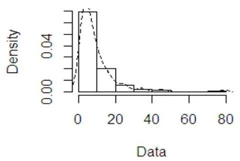
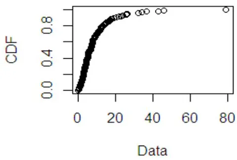
Table 8 shows the parameters estimates obtained from the proposed distribution and it sub distributions

Table 7: Descriptive Statistics Bladder Cancer Patient The Summary statistics of data in table 6 displayed in table 7 shows that the first data set on a bladder cancer patient is over-dispersed and right-skewed, Correlation matrix of TIIHLEL

Min	Max	Mean	SD	Median	Q1	Q3	Skewness	Kurtosis
0.080	79.050	9.366	10.5083	6.395	3.348	11.840	3.2866	15.4831

Notes

1.0000000	0.008513745	-0.999555798	0.006030967
0.008513745	1.0000000	0.006280632	-0.978044473
-0.999555798	0.006280632	1.0000000	-0.004450433
-0.006030967	-0.006030967	-0.004450433	1.0000000

The above correlation matrix indicates the pairs which have negative and positive correlation coefficient depending on the combination of the parameters.

Table 8: Maximum Likelihood Estimates of Parameters and their Standard Errors for Bladder Cancer Patient

	Estimated Parameter
Distributions	$\hat{\alpha}$	$\hat{\beta}$	$\hat{\lambda}$	$\hat{\theta}$
TIIHLEL	8.0874(34.3684)	0.0161(0.0108)	0.2017(0.8573)	7.4603(4.2817)
TIIHLBX	0.1758(0.6831)	0.0432(0.0039)	2.7817(10.8111)
TIHLBX	0.1758(0.6831)	0.0432(0.0039)	2.7817(10.8111)
TIIHLE	1.5988(0.2032)	0.1454(0.0149)
EE	1.2186(0.1489)	8.2466(0.9228)
E	6.0891(0.3999)

Table 9: Goodness-of-fit Statistics, Log-likelihood and Information Criteria for Bladder Cancer Patient

Distribution	AIC	BIC	LL	$A^*$	$W^*$	K-S
TIIHLEL	828.4315	839.8397	-410.2158	0.1971	0.0279	0.0385
TIIHLBX	847.7955	856.3516	-420.8978	2.8260	0.5545	0.1242
TIHLBX	847.7955	856.3516	-420.8978	45.9030	9.8390	0.5000
TIIHLE	973.9203	979.6243	-484.9601	5.6365	0.9516	0.1365
EE	830.8943	835.8593	-413.0776	0.7110	0.1272	0.0723
E	1023.348	1026.2000	-510.6739	11.2831	1.9938	0.1792

Table 9 revealed that the TIIHLEE distribution provides a better fit to the bladder cancer patient data than other competitive models, the TIIHLE, HLEE, HLE, and the E distribution. The TIIHLEE distribution has the highest log-likelihood and the smallest K-S, W*, A*, AIC, and BIC values compared to the other models. Although the TIIHLEE distribution provides the best fit to the data and the EE distribution is alternatively good model for the data since it measures of fit value are close to that of the TIIHLEE distribution.

The estimated asymptotic variance-covariance matrix of the TIIHLEL distribution for the bladder cancer patient data is given by

I_{ij}^{-1} = \begin{pmatrix} 1.181187e+03 & 3.178176e-03 & -2.945031e+01 & -0.88750073 \\ 3.178176e-03 & 1.179766e-04 & 5.848234e-05 & -0.04548612 \\ -2.945031e+01 & 5.848234e-05 & 7.349316e-01 & -0.01633609 \\ -8.875007e-01 & -4.548612e-02 & 1.633609e-02 & 18.33346935 \end{pmatrix}

Notes

However, the confidence interval at 95% for the estimate $\hat{\alpha}$ , $\hat{\beta}$ , $\hat{\lambda}$ and $\hat{\theta}$ are (-59.2747, 75.44947), (0.0052, 0.0379), (-1.4786, 1.8819) and (-0.9319, 11.7421) respectively. The confidence interval for the parameters contains zero. Thus, all the estimated parameters of the TIIHLEL distribution were significant at the 5% significance level

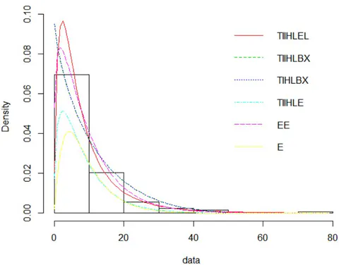
Histogram and theoretical densities Fig. 6: Fit Plot of TIIHLEE Model with other Models for Bladder Cancer Patient

Fig 6 shows the histogram of the bladder cancer data set along with the fitted model. The theoretical density of TIIHLEL distribution has a better spread to the right than other existing models on the data set.

Table 10: Second Data Set

17.88	28.92	33.00	41.52	42.12	45.60	48.80	51.84
51.96	54.12	55.56	67.80	68.44	68.64	68.88	84.12
93.12	98.64	105.12	105.84	127.92	128.04	173.40

Table 10 Represents the number of million revolutions before failure for each of twenty-three (23) deep groove ball bearings in the life tests. The data set was given by Lawless (1982).

Table 11: Summary Statistics of Deep Groove Ball Bearings

Min	Max	Mean	SD	Median	Q1	Q3	Skewness	Kurtosis
17.88	173.40	72.23	37.4804	67.8	47.20	95.88	0.9419	0.4889

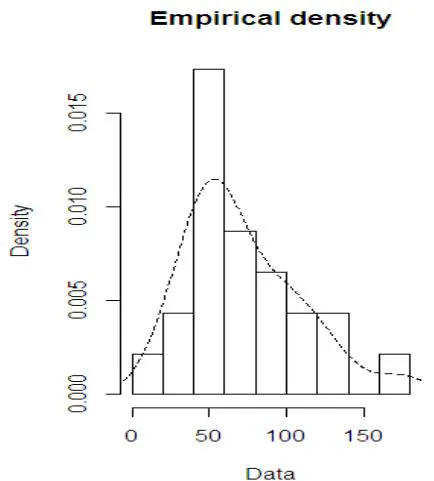
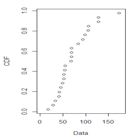
figure 5 shows that the data set is right skewed. Cumulative distribution

Fig. 7: Histogram and CDF Plots of an Empirical Distribution for deep groove ball bearings

Figure 7 shows the empirical plot of data set in table 10 which is right skewed Correlation matrix of TIIHLEL Distribution

1.0000000	0.06631924	-0.93493249	0.05851001
0.06631924	1.0000000	0.06631901	-0.70226965
-0.93493249	0.06631901	1.0000000	0.05850993
0.05851001	-0.9368186	0.05850993	1.0000000

The above correlation matrix indicates the pairs which have negative and positive correlation coefficient depending on the combination of the parameters.

Table 12: Maximum Likelihood Estimates of Parameters and their Standard Errors for Deep Groove Ball Bearings Table 12 shows the parameters estimates obtained from the proposed distribution and it sub distributions.

	Estimated Parameter
Distributions	$\hat{\alpha}$	$\hat{\beta}$	$\hat{\lambda}$	$\hat{\theta}$
TIIHLEL	2.6919(2.9647)	0.0056(0.0018)	2.5214(2.7769)	6.3149(1.8623)
TIIHLBX	0.5337(3.1771)	0.0119(0.0017)	2.7063(16.1097)
TIHLBX	0.5337(3.1771)	0.0119(0.0017)	2.7063(16.1097)
TIIHLE	5.7321(2.2575)	0.0332(0.0065)
EE	5.2936(2.0542)	30.9302(6.1506)
PARETO	0.2399(0.0500)

Table 13: Goodness-of-fit Statistics, Log-likelihood and Information Criteria for Deep Groove Ball Bearings

Distribution	AIC	BIC	LL	A*	W*	K-S
TIIHLEL	438.8069	446.2917	-215.4034	0.1681	0.0241	0.0740
TIIHLBX	452.346	457.9596	-223.1730	1.5815	0.2769	0.1572
TIHLBX	452.346	457.9596	-223.1730	15.6856	3.3333	0.5000
TIIHLE	439.8658	448.6082	-217.9329	0.5730	0.0798	0.0963
EE	442.8943	446.6367	-219.4471	0.8629	0.1301	0.1169
PARETO	593.7705	595.6417	-295.8853	16.9144	3.6482	0.5483

Notes

The TIIHLEL distribution provides a better fit to the data set compared to the other models. From Table 13, the TIIHLE distribution has the highest log-likelihood and the smallest K-S, W*, A*, AIC, and BIC values compared to the other fitted models.

The asymptotic variance covariance matrix for the estimated parameters is

I_{ij}^{-1} = \begin{pmatrix} 8.7894149234 & 3.583368e-04 & 7.6968938753 & 0.32304036 \\ 0.0003583368 & 3.321573e-06 & 0.0003356335 & -0.00238354 \\ -7.6968938753 & 3.356335e-04 & 7.7109968035 & 0.30257389 \\ 0.3230403634 & -2.383540e-03 & -0.3025738897 & 3.46811291 \end{pmatrix}

The confidence interval at 95% for the estimate $\hat{\alpha}$ , $\hat{\beta}$ , $\hat{\lambda}$ and $\hat{\theta}$ are (-3.1189, 8.5028), (0.0055, 0.0167), (-2.92126, 7.9641) and (2.6648, 9.9649) respectively.. It can be observed that the confidence intervals for the parameters do not contain zero, this shows that all the parameters of the TIIHLEL distribution were significant at the 5% significance level.

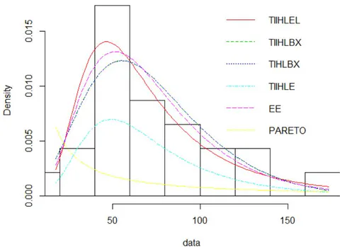
Histogram and theoretical densities Fig. 8: Fit Plot of TIIHLEL Model with other Models for Deep Groove Ball Bearings Discharge

Fig 8 also shows the histogram of the Deep Groove Ball Bearings data set along with the fitted model. The theoretical density of TIIHLEL distribution has a better spread to the right than other competing models on the data set.

VIII. CONCLUSIONS

In this study, we have derived, studied the properties and applications Type II Half Logistic Exponentiated Lomax (TIIHLEL). Some structural mathematical properties; Moment Incomplete moments, Probability Weighted Moment, Order Statistic, and Rényi entropy of the derived model are investigated. A simulation study is carried out to estimate the behavior of the shape and scale model parameters. Also, maximum likelihood estimators were investigated. The application of two real-life data set shows that the TIIHLEE strong and better fit as compare to other existing distribution. However, we hope that this distribution will attract wider applications in the areas of sciences and applied sciences.