

I. INTRODUCTION
In nonlinear optimization, quadratic programming is the most simple optimization problem, and its applications have been widely studied [1], which are ranged from engineering [2, 3, 4] to business [5, 6, 7]. For allocating resources, the quadratic programming problem, which has an objective function in the quadratic form and subject to a set of constraints, is employed. Consequently, a quantitative decision could be made by referring to the optimal solution obtained from solving the quadratic programming problem, especially with the fuzzy parameters [8, 9, 10]. Also, the computational techniques for solving the quadratic programming problem under the probabilistic environment [11] and the related robust solution [12] are actively studied.
By the use of quadratic programming, this paper aims to discuss the uncertain parameters, which are presented in quadratic programming problem without constraints. In doing so, a general unconstrained quadratic programming problem is considered, and the analytical solution is discussed. In the uncertain parameters, the analytical solution does not exist unless an assumption of knowing these uncertain parameters is made. Hence, the quadratic programming problem could be handled practically, where the uncertain parameters are assumed to be normally distributed. On this basis, the simulation is performed on the uncertain parameters to give a possible optimal solution to the quadratic programming problem.
The paper is organized as follows. In Section 2, the unconstrained quadratic programming problem is described in general, and the analytical solution is provided. In Section 3, the presence of the uncertain parameters in the quadratic programming problem is taken into consideration. These parameters are assumed from the normal distribution, and the simulation is made to identify these parameters. The solution procedure is then summarized. In Section 4, an illustrative example is further discussed. Finally, a concluding remark is made.
II. PROBLEM STATEMENT
Consider a general unconstrained quadratic programming problem [13, 14], given by
Minimize
where is an n-vector of decision variables, is a symmetry positive definite matrix, is an n-vector of coefficients, and is a constant. Under the certainty situation, the values for parameters A, b, and c are known and complete. Thus, to determine the optimal solution of the problem in (1), the first-order necessary condition [15, 16],
is derived from giving
Note that (3) is a system of linear equations, and its solution can be obtained from
However, the analytical solution given by (4) would not exist if the parameters A, b, and c are unknown and incomplete information. From this point of view, a computational procedure is required to handle these uncertain parameters, so the unconstrained quadratic programming could be solved in practice.
III. OPTIMIZATION MODELLING APPROACH
Now, assume that the uncertain parameters are normally distributed, where mean and covariance are known necessarily . Therefore, a simulation procedure is properly performed in handling these uncertain parameters. It is followed by using any optimization gradient techniques to solve the unconstrained quadratic programming problem for the possible optimal solution.
a) Uncertain Parameters Simulation
Suppose the values of the elements in the matrix and the vector , for , and , are unknown, and these values are defined in the uncertainty set U, that is,
where
are assumed to be normally distributed with is the mean vector and is the covariance matrix for the elements of the matrix , and is the mean vector and is the covariance matrix for the elements of the vector .
By considering the simulation of the normal distribution, the uncertain parameters are determined from
where is the confidence level, is the z-score at the confidence level for the parameters , and is the z-score at the confidence level for the parameters .
b) Calculation Solution Procedure
After the simulation is carried out to the uncertain parameters, the unconstrained quadratic programming problem is solved by using the optimization gradient approach , which is given by
where represents the step size at the iteration number k, calculated from
and
is the gradient function at , that is,
From the discussion above, the calculation procedure for solving the unconstrained quadratic programming problem, where uncertain parameters exist, is summarized as follows.
Algorithm 1
Data A, b, c, , , , and . Set the iteration number k = 0, the initial value , the tolerance , and the number of simulation trials n.
Step 1 Simulate the uncertain parameters and , respectively, from (7) and (8). Step 2 Calculate the gradient from (12).
Step 3 Compute the parameter from (10).
Step 4 Obtain the optimal solution from (9).
Step 4 Evaluate the value of the objective function
Step 5 Update the simulation trial number. If , stop the calculation, else, set , and repeat from Step 1.
Remark
The optimal solution to the unconstrained quadratic programming problem would be different for each simulation cycle. Hence, the simulation values for the decision variable are determined by solving the unconstrained quadratic problem. For this reason, the possible optimal solution shall be preferred in this situation.
IV. ILLUSTRATIVE EXAMPLE
Consider a quadratic programming problem with no constraint [14, 16] given by
This problem is solved by using the risk simulator software [18, 19, 20]. With the complete information of the matrix A and the vector b, the optimal solution is , and the objective function has a minimum value of 1.50.
For the uncertain situation, two cases are further investigated. In Case 1, only the matrix A is assumed to have an uncertain value of entries, while in Case 2, both matrix A and vector b are assumed to have uncertain entries. The number of simulation trials is set to 500, and the number of optimization runs is set to 20.
Case 1:
Assume that the parameters in matrix A have mean and standard deviation given by
Suppose and c=10 are known.
Suppose and c=10 are known. The simulation results for the decision variables and the objective function are shown in Table 1 and Table 2.
| Decision Variable | Initial Value | Final Value | Mean Value |
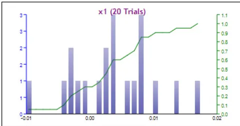
| -0.00105 | 0.00068 | 0.000277 | |
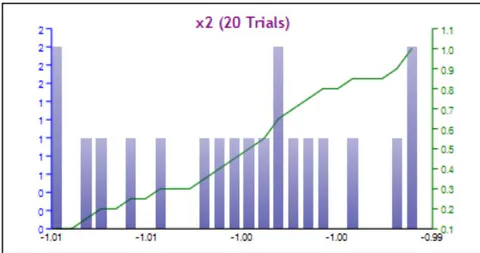
| -1.00107 | -1.01098 | -1.00118 | |
| -0.99732 | -0.99795 | -0.99865 |
| Objective Function | Initial value | Final Value | Iteration Numbers |
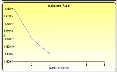
| f | 1.46040 | 1.46006 | 6 |
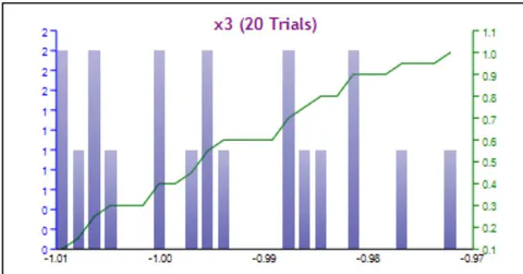
The graphical result for the objective function is shown in Fig. 1, while the simulation values for decision variables , and are shown in Figs. 2, 3, and 4, respectively. Notice that the figures' bars represent the respective simulation values, and the lines show the relative cumulative distribution values.
Case 2:
To observe the possible results that might be obtained under the uncertainty, consider the entries of the matrix A has mean and covariance as given in (14), and assume the entries of the vector b is normally distributed with mean and variance given by
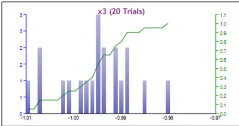
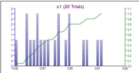
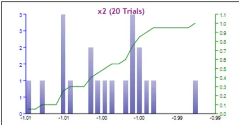
Table 3 and Table 4 show the simulation results for the decision variables and the objective function, respectively.
| Decision Variable | Initial Value | Final Value | Mean Value |
| -0.01137 | -0.00226 | -0.0019 | |
| -1.00806 | -0.99402 | -1.00016 | |
| -0.97891 | -0.98902 | -0.99607 |
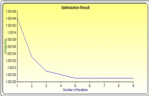
| Objective Function | Initial value | Final Value | Iteration Numbers |
| f | 1.63204 | 1.63127 | 9 |
The graphical result of the objective function and the simulation values for the decision variables , , and are shown in Figs. 5, 6, 7, and 8, respectively.
Therefore, assuming the uncertain parameters are normally distributed and applying the simulation procedure, the unconstrained quadratic programming problem could be solved in advance. The possible optimal solution obtained mainly depends on the simulation performed to the uncertain parameters and the gradient approach used.
V. CONCLUDING REMARKS
This paper has discussed the unconstrained quadratic programming problem with the presence of uncertain parameters. It is assumed that these parameters are normally distributed, and their values are determined from the simulation process. Accordingly, the unconstrained quadratic programming problem is solved by using the optimization gradient approach. The resulted simulation values of decision values are identified to obtain the possible optimal solution to the problem. In conclusion, the computation procedure used could handle the uncertain quadratic programming problem practically. For future research direction, it is recommended to cover the constraints, both for equality and inequality constraints, in solving the quadratic programming problems.
ACKNOWLEDGMENT
The authors would like to thank the Ministry of Education Malaysia (MOE) for supporting this research under the Fundamental Research Grant Scheme Vot No. FRGS/1/2018/STG06/UTHM/02/5 and partially sponsored by Universiti Tun Hussein Onn Malaysia.