## I. INTRODUCTION Energy utilization in structures is perhaps one of the quickest developing areas. Roughly $41\%$ of the all-out energy in Europe is consumed by structures (families and administrations) [1]. Studies and states' mandates about limiting energy utilization and utilizing sustainable power expanded consistently with the decrease of petroleum derivatives, the line contacts with eastern nations like Russia, and the increment of different natural issues. In light of this, the European association, with a new order [2], has the objective to raise EU energy utilization created from sustainable assets to $20\%$, to lessen by $20\%$ the EU ozone-depleting substance discharges and to improve by $20\%$ the EU's energy productivity. This implies speculations to requalify old structures, new nation regulations, and energy analysis, yet in addition, new productivity frameworks from the pre-owned apparatuses. Determining energy requests has become one of the significant exploration fields in the energy divisions since it can assist with gassing utility organizations and families. Gas utilities purchase gas from pipeline organizations on an everyday basis, so they need to know the necessities ahead of time to be cutthroat. Organizations and families have the point of decreasing energy utilization and increment effectiveness. Lately, enormous organizations like Google have also shown their premium in this new market, creating indoor regulators that consequently control the house environment and putting together choices with respect to the client's timetable. Home, an organization procured by Google, pronounced that clients saved the $11.3\%$ of AC-related energy use without compromising solace [3], because of the programmed learning carried out in their indoor regulators. On the off chance that, on the one hand, the programmed indoor regulator program setting in light individuals conduct can assist them with setting aside cash, peculiarity location can diminish the energy utilization. It is displayed by [4] and [5], that business structures consume from $15\%$ to $30\%$ more energy than needed due to ineffectively kept up with, corrupted, and inappropriately controlled hardware. These inconsistencies can turn out to be simply fixable issues with a dependable shortcoming location and conclusion (FDD) framework. In this paper, an automatic outlier detection system is proposed, where days/hours with abnormally high and low gas consumption are labeled and reported to the building manager. He can further analyze and fix the HVAC system, minimizing the energy waste caused by the outliers. Gas consumption is very irregular and not easily predictable with classic methods. The outlier detection system presented is based on predictions made by a hybrid ARIMA-ANN, which can model linear and non-linear behavior of the data with very reliable results and a comparison between the predicted value/trend and the actual one to find outliers. Since the definition of outlier is highly application dependent, in section II they are defined. In the same section, ANNs and ARIMA are briefly explained because they will be lately used in the proposed solution (section IV), based on a gas consumption forecaster. In section III some related works are discussed. In section V, some experiments on synthetic and real data are shown. Section VI presents some future ideas for the readers based on techniques that the author didn't have the time to apply. ## II. BACKGROUND ### a) What is an outlier An exception, by definition [6], is a perception that goes astray fundamentally from different perceptions, so it makes doubt that various elements made it. Regardless of this overall definition, the more fitting approach to characterizing exceptions is exceptionally application-subordinate since even similar situations might require various judgments of anomalies. In this paper, exceptions are firmly connected with the issue of time-series gauging since anomalies are proclaimed based on deviations from expected (or estimated) values. In this unique circumstance, a worth is viewed as an exception due to its relationship to its connected information (contextual exception [7] or contingent oddities [8]). An unexpected pinnacle (fig. 1) in a period series is a contextual exception in light of the fact that its worth is totally different from the upsides of its nearby items. At the point when a gathering of focuses are proclaimed exceptions, it is alluded as collective peculiarity or anomaly [7]. It initially shows up at a point, and afterward, it influences the qualities promptly close to it. Sooner or later, this impact vanishes, passing on the time series to a typical way of behaving. This situation is normally difficult to identify. Outliers can have distinct main reasons: 1. Defective system (e.g., a defective heater in a room). 2. Bad human behavior (e.g., people who leave open the window in a room while the system is trying to heat it). 3. Defective monitoring system, where the system monitors different values from the real one due to a malfunction, computing process errors, or recording negligence. In literature, outliers are also referred to as abnormalities, deviants, novelties or anomalies.  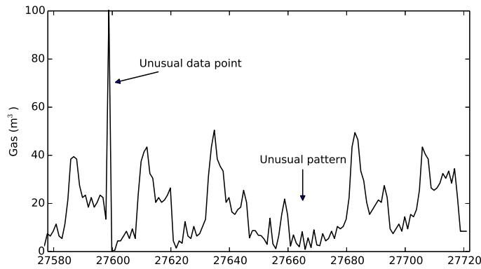Fig. 1: Different Types of Outliers. On the Left an Unusual Data Point is Presented, on the Right an Unusual Pattern of Changes can be Recognized if Compared to the other Days Shape ### b) Artificial Neural Networks Counterfeit Brain Organizations (ANNs) were initially evolved to impersonate the mind's usefulness. There is definitely not a broadly acknowledged definition yet by [9]: "A brain network is a circuit made out of an extremely huge number of straightforward handling components that are neurally based. Every component works just on nearby data. Moreover, every component works nonconcurrently; in this manner, there is no general framework clock." From section II-B, it is feasible to see a completely associated ANN with five sources of info, 3 neurons on the secret layer (purported on the grounds that the ANN resembles a black box), and one result. The data sources are additionally called elements, and they address the attributes to portray the result. The secret neurons will plan this connection. Every association has an initiation that addresses the significance (weight) of the associated neuron. ANNs with something like a 1-stowed away layer can plan nondirect relations. The hidden neurons are usually represented with logistic sigmoid units, which internally calculate the sigmoid function of the inputs, but also with a hyperbolic tangent. Recent findings argued that rectifier units seem to be more biologically plausible [10], and they also seem to perform better in ANNs.  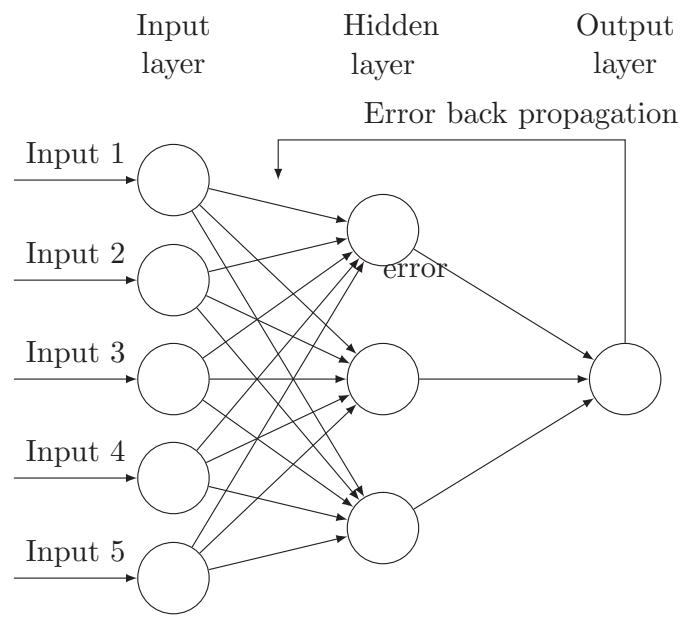Fig. 2: Artificial Neural Network with Backpropagation. Example with 5 Inputs, 3 Hidden Neuron in the First Hidden Layer, and One Output (in the Case of This Paper, the Gas Consumption Value) The ANNs are commonly applied with the Stochastic Gradient Descent algorithm, which tries to find the right weights of each connection to have the right output value. It is usually combined with the Backpropagation algorithm which calculates the error in the output layer and then backpropagates it to the previous layers in order to adjust the weights [11]. More information can be found in [12]. Nowadays, ANNs are a state-of-the-art technique that has many applications. ### c) Autoregressive Models Let $X_{1}, X_{2}, \ldots, X_{t}$ be the values in an univariate time-series. In the Auto-Regressive Moving Average model, the value of $X_{t}$ is defined in terms of the values of the last window of length $p$ and $q$ moving average terms. $$ X_{t} = \sum_{i=1}^{p} \varphi_{i} X_{t-i} + \sum_{i=1}^{q} \theta_{i} \varepsilon_{t-i} + c + \varepsilon_{t}. $$ The left-hand part is called the auto-backward part since it relies upon the past (slacked) values $X_{t - 1}, X_{t - 2}, \ldots, X_{t - p}$, the right-hand part is called moving normally in light of the fact that the blunder at time $t$ is the direct mix of the past mistakes $\varepsilon_t - _1, \varepsilon_t - _2, \ldots, \varepsilon_t - _q$. These techniques are applied to stationary time-series, alleged when the mean, fluctuation, and autocorrelation structure don't change over the long run. Tragically, many time series make occasional impacts or patterns. Specifically, arbitrary strolls, which describe many sorts of series, are non-fixed. Differencing the information focuses can frequently change a non-fixed time series into a fixed one. In view of the Crate Jenkins models of the 1970s, ARIMA models are separate, where a series with deterministic patterns ought to be differentiated first, and then an ARMA model is applied. ARIMA models are typically referenced as ARIMA (p, d, q), to show the ARMA boundaries and the $d$ request of difference. ARIMA models are likewise fit for displaying a lot of information. $$ \operatorname{ARIMA} (p, d, q) (P, D, Q) _ {m} $$ where $m$ is the quantity of periods per season. The capitalized documentation is utilized for the occasional pieces of the model, and the lower-case documentation for the nonoccasional pieces of the model. The decision of the boundaries $p, d, q$ is exceptionally application ward, and it depends on a hypothesis that is past the extent of this paper. More data can be found in [13]. ## III. RELATED WORK Since this paper declares outliers based on deviations from the expected (or forecast) value, this section is divided into related work in forecasting and outlier detection. ### a) Outlier Detection Outlier detection systems are a wide range of areas, from introduction detection systems to fraud detection systems, law enforcement systems to earth science anomaly detection systems. Outlier detection can be supervised when available data is labeled indicating previously known examples of anomalies, semi-supervised, where only examples of normal data or anomalies are available, or unsupervised, where previous examples of interesting anomalies are not available. Typically, most of the unsupervised outlier mechanisms use a measure of outlierness of a data point, such as sparsity of underlying region, nearest neighbor distance, or the fit to underlying distribution [7]. In these cases, a data point is unusual due to one or more variables rather than a specific one (like in the supervised methods). In energy consumption outlier detections, literature is usually based on the Gaussian error theory, stating that when the measurement accord with normal distribution, the probability that the residual falls in three times the variance is more than $99.7\%$. Therefore, the residuals falling outside can be considered outliers. In [14], the author further improved this system by considering a rolling window median, which seems to improve the results when the distribution is not fixed. Supervised methods are usually based on classifications using trees, ANNs, and other different algorithms, thanks to the presence of previous examples of anomalies. In the energy consumption field, unsupervised methods are usually based on clustering, where an algorithm tries to find similarities between points/trends and cluster them into groups, calculating the distance between them. A cluster is considered good when the intra-cluster distance is minimized, and the intra-cluster distance is maximized. Popular methods in this group are kmeans, one-class SVM, and self-organizing maps. For example, in [15], some clustering methods, like CART, $k$ -means, and DBScan, were applied to detect outliers in the office lighting energy consumption. The author showed different techniques applied with the Generalized Extreme Studentized Deviate (GESD) and listed some irregularities found. He also stated that the clustering methods were not able to detect faults strongly related to time variables. Clustering methods are very difficult to apply in timeseries data, and the results are usually poor. For this reason, this paper will build a prediction algorithm, where outliers are declared based on deviations from expected (or forecast) values. The more accurate the predictor, the more abnormal data points will be detected. ### b) Forecasting Traditionally, several techniques have been used for energy use forecasting, but short-term, medium-term, and long-term energy forecasting needs to be differentiated. The former usually refers to prediction with a horizon of hours or days; the second refers to weeks, and the latter refers to a monthly or annual horizon. Long-term forecasting usually deals with data that rarely presents significant distortions and irregularities, so they have a small effect on the overall value. On the contrary, short-term forecasting has to deal with irregularities and sudden changes in values (due to weather changes, human behavior, etc.). There are essentially five types of prediction models [16]: Engineering methods, Statistical methods, Artificial Neural networks, Support Vector Machines, and Grey models. Engineering methods use physical principles to calculate thermal dynamics and energy behavior of the building, Statistical methods build empirical models to apply a regression to a time series of values, Neural networks try to predict energy using an artificial intelligence network of interconnected neurons, Support vector machines are based in a machine learning algorithm and Grey models apply a mixture of the models. All the principal methods are extensively reviewed in [16] and [17]. Several techniques have been traditionally applied for energy use forecasting, and among the statistical methods, Kalman filtering and ARIMA/ARMAX time-series techniques are the most famous. The first reports about applications of Artificial Neural Networks (ANNs) were published in the early 1990s [18]. Since then, the number of publications increased steadily. Kalogirou et al. [19] used back propagation neural networks to predict the required heating load of 225 buildings; Ekici and Aksoy used the same model to predict building heating loads in three buildings. Nizami and Al-Garni [20] tried a simple feedforward NN and related the electric energy consumption to weather data and population, Taylor and Buizza [21] used an ANN with weather data (51 variables) to predict load of 10 days ahead. Gonzales [22] built an ANN to predict hourly energy consumption. Some researchers tried to specialize the ANNs: Neto and Fiorelli [23] compared generic ANNs with working days ANNs and week-end ANNs, Lazzerini and Rosario [24] specialized them to predict electric lighting with weather data. Some researchers have also tried to apply a hybrid model to increase the performance of the ANN. One example above all is [25] which applied a hybrid ARIMA and neural network model to forecast electricity use, another one is [26] who improved the previous one. This paper is based also on his work. Until now, only electric forecasting was presented because the majority of the existing forecasters are related to electric forecasting. There are only a few of them are about natural gas forecasting: Brown et al.[27] built one of the first predictors for natural gas consumption, and Khotanzad et al. [28] developed a two-stage system ANN with very good results. Even if ANNs might outperform traditional methods, the researchers are still not convinced about the results of ANNs in this field. Nevertheless, it is also stated that "a significant portion of the ANN research in forecasting and prediction, lacks validity" [29] and that most of the papers seem misspecified models that had been incompletely tested (no standard benchmarks, no synthetic data, etc.) [17]. This paper will try to avoid these mistakes. It also needs to be pointed out that ANNs are multistep ahead forecasters, while Auto-Regressive methods are potentially useless in long ahead data points. ## IV. PROPOSED SOLUTION As stated before, this paper proposes a regression algorithm in which outliers are declared based on deviations from the expected (or forecast) value. A time-series is a sequence of data-points typically measured at successive points of a uniform time interval $t$ (eq. (1)). $$ \{x \left(t _ {0}\right), x \left(t _ {1}\right), \dots x \left(t _ {i}\right), x \left(t _ {i + 1}\right) \dots \} \tag {1} $$ where $x$ is the value and $t$ the time. Time-series forecasting is about predicting future values given past data (eq. (2)). $$ \hat {x} (t + s) = f (x (t), x (t - 1) \dots) \tag {2} $$ where $s$ is the step size. A multivariate time-series is a $(n\times 1)$ vector of $n$ time-series variables. It can be seen that in academic and industry research, linear regression-based systems are the standard "de facto" of energy forecasting, and in recent works, this problem is treated by combining weather forecast data. However, this relationship is clearly nonlinear [17]. Consequently, even if some papers have acceptable results with measured datasets, these systems cannot adequately capture the relationship in all the situations and data. Since ANNs are the state-of-the-art technique of many machine learning problems where there is complex nonlinear hypotheses, the proposed solution is composed of a multilayer feedforward neural network with backpropagation. Table I: Buildings used <blockquote><table><tr><th>Building name</th><th>Date interval</th><th>Number of rows</th></tr><tr><td>Hva 740 - NTH</td><td>01/2008 - 03/2014</td><td>54.725</td></tr><tr><td>Hva 761 - KMH</td><td>01/2009 - 09/2013</td><td>40.407</td></tr><tr><td>Hva 882 - WBW</td><td>01/2008 - 03/2014</td><td>54.647</td></tr></table></blockquote> <blockquote><table><tr><th>Building name</th><th>Date interval</th><th>Number of rows</th></tr><tr><td>Hva 740 - NTH</td><td>01/2008 - 03/2014</td><td>54.725</td></tr><tr><td>Hva 761 - KMH</td><td>01/2009 - 09/2013</td><td>40.407</td></tr><tr><td>Hva 882 - WBW</td><td>01/2008 - 03/2014</td><td>54.647</td></tr></table></blockquote> ### a) Experimental Data Ebatech gathers the energy utilization datasets utilized in various structures of the Hogeschool van Amsterdam. The Universiteit van Amsterdam gave these datasets to this undertaking. These structures are situated in Amsterdam, the capital city of The Netherlands. This city has a sea environment like Britain, firmly impacted by the North Ocean. Winters are genuinely cold, and summers are seldom sweltering, according to European guidelines. Amsterdam is described by the normal presence of downpours and wind, and the weather patterns change frequently. Ebatech gathered various sorts of elements in every structure, with various granularity. For this undertaking, three structures are utilized: Hva 740 - NTH, Hva 882 - WBW, and Hva 761 - KMH. In these structures, the organization gathered the energy utilizations and the gas utilizations as different factors. It should be noted that gas is utilized exclusively to warm the structures. The weather data was collected by KNMI¹ in Schipol, the Amsterdam airport 16 km far from the tested buildings. The dataset, findable on the website, consists of over 21 variables collected hourly. The proposed solution only uses a few of them, as explained in the section IV-B, and they are used as forecast values: the measured weather conditions are linked to the previous hour of energy consumption. It is necessary to consider that there will be an error in the built model since the weather data is collected in a different location from the building's positions, and in practice, the error will be larger than those obtained in this simulation due to the effect of the weather forecast uncertainty [30], [31]. The advice is to keep it in mind before applying the methods contained in this paper with days forecasting. The gas consumption data is highly seasonal: daily and weekly cycles are quite perceptible, as it can be seen from fig. 4 and fig. 3. From the latter, the weekly behavior is clear: the last two days of the week (Saturday and Sunday) are completely different from the others, and Monday seems a bit different from the rest of the days. Every day, around 4:00-5:00 AM, the system seems to react by turning on the heating system, whereas in the previous hours of the night, it seems only to keep a minimum temperature. The system reveals to us that after a couple of hours, it decreases the consumption again. In fig. 4 the Temperature has a clear daily/hourly relation with the gas consumption while in fig. 5 the electric consumption is shown to be very smoothed and more regular than the gas one.  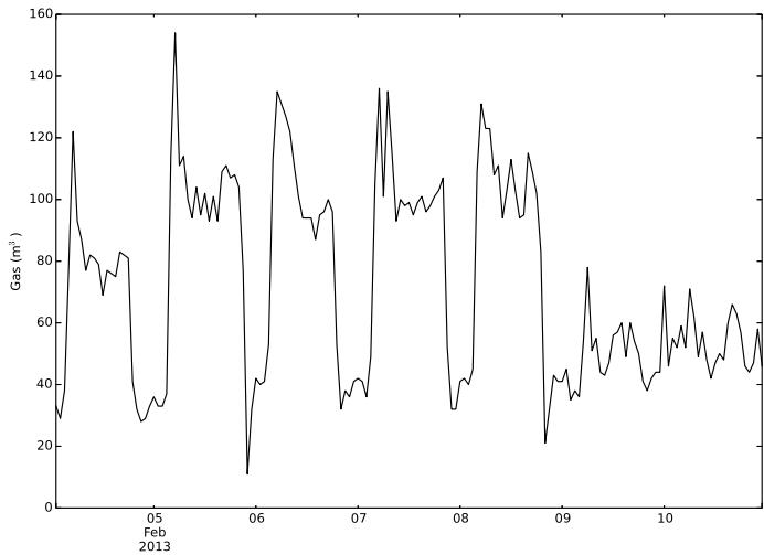Fig. 3: Typical weekly and daily gas consumption behavior in building 740NTH. The weekly pattern can be noticed by observing that the last two days of the week (Saturday and Sunday) have a completely different shape than the others. 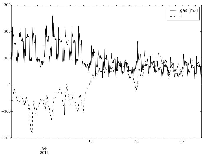During the week, the daily behavior is very similar, with one peak around 4:00-5:00 AM  Fig. 4: Typical Monthly gas Consumption Behaviour in Building 740-NTH and its Relation with the Temperature on Building 740-NTH Missing and repeated data points represent some problems in the data collection that will be further investigated.  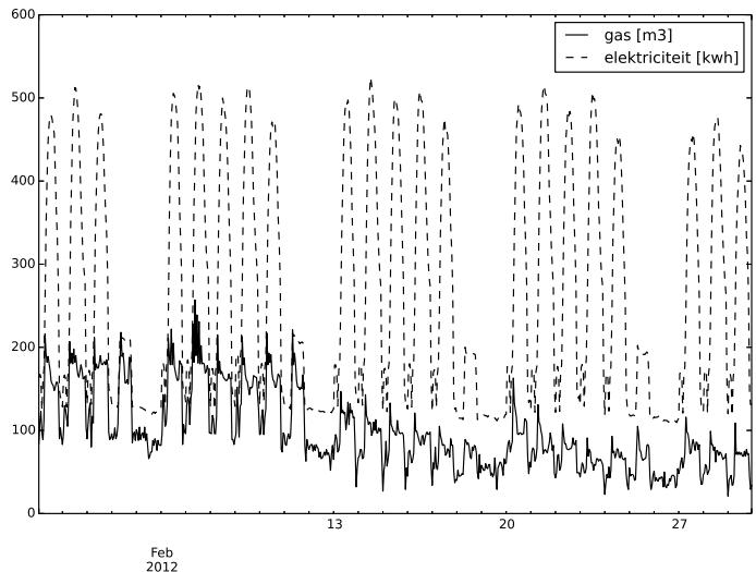Fig. 5: Relation between Electric and Gas Consumption in Building 740-NTH ### b) Artificial Neural Network Forecaster Time series are characterized by more or less complex dependencies: Known dependencies like datetime dependencies. Hidden dependencies include the behavior of the HVAC system (when it starts, when it raises the temperature, etc). Short/long -term dependencies between variables. Data scientists and experts are focused on known dependencies, while the proposed ANNs will be focused on the hidden ones. The short/long-term dependency is realized by a moving window containing a "memory" of the previous states for the interesting variables, using a Tapped delay line memory [32]. These memories form a new set of states- $$ \{\bar {x} _ {1} (t), \bar {x} _ {2} (t), \dots \bar {x} _ {n} (t) \} $$ from the original states $$ \{x (1), x (2) \dots x (n) \} $$ where $\vec{x}_i(t) = x(t - i + 1)$. The window types will be explained later in this section. Since the value to predict is time-dependent, the first element to consider is adding the time feature. Energy consumption depends on the hour of the day but also on the day of the week and the seasonality of the year (month and day of the year) (as explained in section IV-A1, fig. 4 and fig. 3). The day of the week is a number from 0 to 6, where 0 is Monday and 6 is Sunday. Since the behavior of the holidays was considered similar to the weekends (particularly similar to Sundays), a function encoded all the holidays as weekend days². In the future, this can be improved by asking for a timetable list for the buildings, indicating when these are closed. The day of the year is a number between 0 and 366, and the first one is the first of January. All these date-time features by means of their sine and cosine values as usual, reported in literature [33], [34], [22]. This transforms the time component into a cyclic feature that spans a fixed length (a single day for the hour), and it is bounded in $[-1,1]$. Another added feature was the current system load, which is the energy consumption at the $k$ state when the load at $k + 1$ needs to be predicted. This was believed to be an important measure for determining building usage and holidays. Many elements influence the energy needs of structures. These variables can be separated into three principal bunches, specifically the physical environmental, the artificial planning parameters, and the human warm discomfort. The first is made out of weather conditions related to boundaries like open-air temperature, wind speed, sun-powered radiation, and so forth. The artificial planning parameters are connected with the structure development: straightforwardness proportion, direction, and so on [35]; however, these factors were inaccessible in the dataset. The human impression of warm discomfort is connected not exclusively to the temperature but also to different factors, for example, relative stickiness, illumination, and wind speed. Regardless of whether this large amount of information was accessible, the main climate factors found were the temperature and the breeze speed. The framework utilization was accepted to be connected with the distinction of the open air temperature between two moments (eq. (3)), addressing a positive/negative difference in the outer natural circumstances. $$ \Delta T _ {k + 1} = T _ {k + 1} - T _ {k} \tag {3} $$ where $T_{k+1}$ is the predicted temperature for the period $k + 1$ and $T_k$ is the value measured in the instant $k$. It needs to be noted that the real behavior of the system was unknown, so it was not possible to know if this change would have an immediate effect on the HVAC system and/or its reaction time. Gas usage has a daily cycle but there are also secondary weekly and annual cycles that the ANN may not be able to capture. Gas usage $u(t)$ is defined as $u(t) = s(t) + f(t) + r(t)$ $$ u (t) = s (t) + f (t) + r (t) $$ where $s(t)$ is the seasonality at time $t$, $f(t)$ is the trend and $r(t)$ is called remainder, irregular component or difference. The time series were analyzed by the STL decomposition by LOESS [36](fig. 6), which decomposes a time series into seasonal, trend, and irregular components by an additive method. Since the ANN is interested in the remainder and the trend can be found from the historical part, the daily, weekly, and yearly remainders were added as features. For the same reason also, the Temperature, the wind speed, and the electric consumption were decomposed by the STL decomposition, resulting in a stationary time series added to the input.  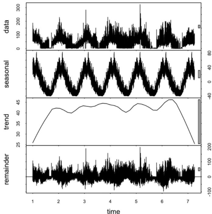Fig. 6: Yearly STL Decomposition by LOESS in Building 740-NTH In Zhang et al. [37], it is expressed that ANN models truly enjoy benefits while managing a lot of verifiable burden information with non-direct trademarks. Yet, the scientists ignored the straight relations, including the information. Hence a cross breed approach is proposed, where the ANN will be helped in direct guaging by the famous strategy ARIMA (autobackward coordinated moving midpoints), generally known as the Container Jenkins approach. To apply ARIMA, the time series was handled iteratively with a moving window of 21 days where the ARIMA model was fitted. After the fitting, the upsides of the following 24 hours were determined prior to moving the window and doing the same for the following day. The occasional ARIMA fitting was finished by the assistance of the Figure R bundle [38] and its auto.arima technique, which finds the best ARIMA $(p,d,q)(P,D,Q)_m$ boundaries by looking at the Akaike data criterion (AIC) of the tried models. Only for the peruser interest, the most fitted model was ARIMA $(3,0,3)(2,0,1)_{24}$. An ARIMA model with temperature sham factors was tried. However, it did not advance the ANN: the least complex models were liked. Taking into account the points made in this section, the ANN is predicting the gas consumption "seeing" without knowing its shape and its behavior in the previous hours/days. This limit is surpassed by some rolling windows, which will somehow simulate the Recurrent neural networks' behavior. Two rolling windows were created for the gas consumption, memorizing the sum and the peak load of the previous five hours, and two moving rolling windows were created for the STL yearly residuals, memorizing sum and peak of them. Table II: Ann Features <table><tr><td>Variable</td><td>Data</td></tr><tr><td>Electricity load</td><td>E(t)</td></tr><tr><td>Hour</td><td>sin(2π(h)/24); cos(2π(h)/24)</td></tr><tr><td>Week day</td><td>sin(2π(wDay)/6); cos(2π(wDay)/6)</td></tr><tr><td>Month</td><td>sin(2π(mon)/12); cos(2π(mon)/12)</td></tr><tr><td>Year day</td><td>sin(2π(d)/366); cos(2π(d)/366)</td></tr><tr><td>Temperature</td><td>T(t)</td></tr><tr><td>Gas peak&#x27;</td><td>max1≤k≤5 G(t-k)</td></tr><tr><td>Gas sum&#x27;</td><td>∑i=15 G(t-i)</td></tr><tr><td>Gas mean&#x27;</td><td>1/288 ∑i=1288 G(t-i)</td></tr><tr><td>Gas peak&#x27;&#x27;</td><td>max1≤k≤24 G(t-k)</td></tr><tr><td>Gas sum&#x27;&#x27;</td><td>∑i=124 G(t-i)</td></tr><tr><td>Electricity peak&#x27;&#x27;</td><td>max1≤k≤5 E(t-k)</td></tr><tr><td>Electricity sum&#x27;&#x27;</td><td>∑i=15 E(t-i)</td></tr><tr><td>Temp peak</td><td>max1≤k≤5 T(t-k)</td></tr><tr><td>Temp sum</td><td>∑i=15 T(t-i)</td></tr><tr><td>Wind speed</td><td>FH(t)</td></tr><tr><td>ΔTk+1</td><td>Tk+1 - Tk</td></tr><tr><td>ARIMA forecast</td><td>forecast(ARIMA(3,0,3)(2,0,1)24)</td></tr><tr><td>STL year res.</td><td>YearRes(t)</td></tr><tr><td>STL day res.</td><td>DayRes(t)</td></tr><tr><td>STL E res.</td><td>Res(E(t))</td></tr><tr><td>ARIMA peak&#x27;</td><td>max1≤k≤5 ARIMA(t-k)</td></tr><tr><td>ARIMA sum&#x27;</td><td>∑i=15 ARIMA(t-i)</td></tr></table> All the features that were not between the limits $[-1,1]$ were scaled to have a faster convergence [39] of the Stochastic Gradient Descent (eq. (4)).(4) $$ x_{i}^{ ext{\prime}} = \frac{x_{i} - \frac{\operatorname*{max}(x) + \operatorname*{min}(x)}{2}}{\frac{\operatorname*{max}(x) - \operatorname*{min}(x)}{2}} \tag{4} $$ where $x_{i}$ is the original value and $x_{i}'$ is the scaled one. Many practical tricks like the shuffling of the elements, the normalization and initialization were taken from [39], [40]. All the process described so far is also called feature engineering and was done almost iteratively, cumulatively introducing and removing features from the model and comparing the performance. Choosing a number of hidden units for the ANN is always a tricky task. As stated by[41]and[42], using early stopping in an oversized Backpropagation ANN, where the number of hidden neurons is higher than the number of features, makes it easier to find the global optimum and avoid bad local optima. For this reason, the number of hidden units was chosen to be greater than$2 \times |features|$and then tested, with training early stopped to prevent overfitting. Architecture: ANNs are trained trying to minimize a cost function of the form $$ E = \frac {1}{N} \sum_ {i = 1} ^ {n} p (r _ {i}) ^ {2} $$ where the error function $p$ is symmetric and continuous, $r_i = Y_i - Y_i'$ is the residual between the actual value and the forecast one, and $N$ is the number of training patterns.  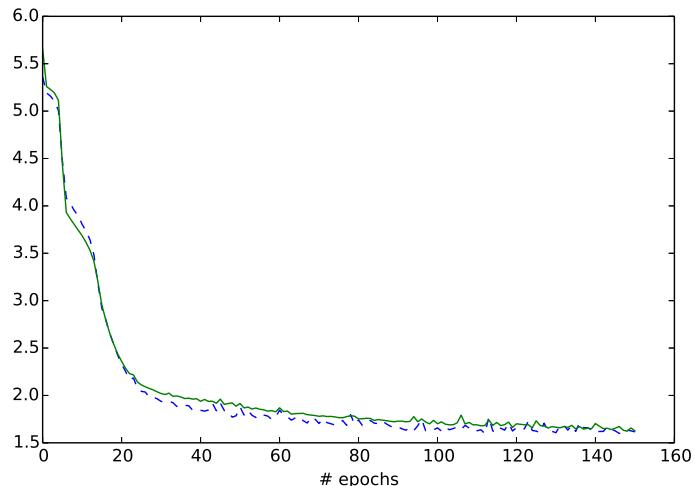Fig. 7: Training Curve of the Hybrid Model with 80 Hidden Neurons --- valid_objective:softmax_re train_objective:softmax_re Using the notations defined above, the most used cost function is based on the Mean Squared Error (MSE), commonly, known in data modeling as the Least Mean Squares (LMS) method. The basic idea of LMS is to optimize the fit of a model with respect to the training data by minimizing the square of residuals $$ p(r) = \frac{1}{2} r^{2} $$ but it is greatly influenced by outliers [43]. In order to control the damage caused by outliers, in this paper the Least Mean Log Squares (LMLS) method (eq. (5)), presented by [43] is used. The ANN will try to minimize the Mean Log Squared Error (MLSE). $$ p(r) = \log\left(1 + \frac{1}{2} r^{2}\right) \tag{5} $$ The ANN is a 1-hidden-layer Multilayer Feedforward ANN with a feedback structure, called Backpropagation. This ANN is composed by Rectifier neurons and one output linear node. Training is done by the Stochastic Gradient Descent algorithm with 10 batch size and is characterized by a learning rate of 0.003 and fixed by a Momentum of 0.05, which could help to increase the speed, avoiding local minima. This project used Python and pandas for the data analysis, Pylearn2 [44] to construct and test the ANN and the R system with the zoo [45] and the Forecast [38] packages for the ARIMA process. ### c) Outlier Detection According to Chebachev's theorem [46], almost all the observations in a data set of system states falls into the interval $[\mu - 3\sigma, \mu + 3\sigma]$, where $\mu$ and $\sigma$ are respectively the mean and standard deviation of the data set, and the data points outside this interval are declared outliers. In this paper the ANN is used to predict the gas consumption, for this reason a point will be considered outlier if it will fall outside the $95\%$ confidence interval³ expressed for the RMSE. If it is assumed that the difference between the actual values $x_{i}$ and the predicted value $x^{\hat{}}_i$ have: $$ \hat {x} _ {i} - x _ {i} \sim \mathcal {N} (0, \sigma^ {2}) \tag {6} $$ - mean zero. - follow a Normal distribution (it is assumed that it holds for the large amount of data utilized). - and all have the same standard deviation $\sigma$ $$ \hat {x} _ {i} - x _ {i} \sim \mathcal {N} (0, \sigma^ {2}) \tag {7} $$ it is possible to say that eq. (7) follows a $\chi^2_n$ distribution with $n$ degrees of freedom. Which means: $$ P \left(\chi_ {\frac {\alpha}{2}, n} ^ {2} \leq \frac {n \mathrm {R M S E} ^ {2}}{\sigma^ {2}} \leq \chi_ {1 - \frac {\alpha}{2}, n} ^ {2}\right) = 1 - \alpha \tag {8} $$ $$ \Leftrightarrow P \left(\frac{n\mathrm{RMSE}^2}{\chi_ {1 - \frac{\alpha}{2}, n}^2} \leq \sigma^2 \leq \frac{n\mathrm{RMSE}^2}{\chi_ {\frac{\alpha}{2}, n}^2}\right) = 1 - \alpha \tag{9} $$ $$ \Leftrightarrow P \left(\sqrt{\frac{n}{\chi_ {1 - \frac{\alpha}{2}, n}^2}}\mathrm{RMSE} \leq \sigma \leq \sqrt{\frac{n}{\chi_ {\frac{\alpha}{2}, n}^2}}\mathrm{RMSE}\right) = 1 - \alpha \tag{10} $$ Therefore $$ \left[ \sqrt {\frac {n}{\chi_ {1 - \frac {\alpha}{2} , n} ^ {2}}} \mathrm {R M S E}, \sqrt {\frac {n}{\chi_ {\frac {\alpha}{2} , n} ^ {2}}} \mathrm {R M S E} \right] \tag {11} $$ ## V. EXPERIMENTAL EVALUATION The ANN has been prepared with early halting, with a decent number of preparing ages (stages) or halting the preparation when the approval blunder rate was expanding. Every one of the outcomes showed is obtained from k-crease cross-approval strategies, where the organization was prepared $k$ times, each time leaving out a subset of information from preparing to test the ANN. The consequences of the $k$ tests were partitioned by $k$. The organization is constantly prepared with $70\%$ of the information, $15\%$ is utilized for approval and the other $15\%$ for testing. Albeit most of the Mean Outright Rate Blunder (MAPE) is viewed as a norm for looking at the nature of the model expectation of energy load, it is a satisfactory mistake measure provided that the misfortune capability were direct and ongoing investigations exhibited it isn't [19][47]. Besides, the rate of blunder is limitless on the off chance that there are no qualities on the series, continuous in discontinuous information and in utilization information, and it puts a heavier punishment on certain mistakes than on regrettable mistakes [48]. In light of these impediments, this paper will just consider the minimization of the Root Mean Square Mistake (RMSE), which punish huge blunders, as proposed in [49]. As recommended in [17], for each analysis, likewise the Mean Outright Blunder (MAE) will be determined. $$ \mathrm{MAPE}^{4} = \frac{1}{n} \sum_{i=1}^{n} \frac{|Y_{i} - \hat{Y}_{i}|}{Y_{i}} \times 100 $$ $$ \mathrm {R M S E} = \sqrt {\frac {1}{n} \sum_ {i = 1} ^ {n} \left(\hat {Y _ {i}} - Y _ {i}\right) ^ {2}} \tag {13} $$ $$ \mathrm {M A E} = \frac {1}{n} \sum_ {i = 1} ^ {n} \left| \hat {Y _ {i}} - Y _ {i} \right| \tag {14} $$ where $Y^{\wedge}$ is the vector of the $n$ predictions and $Y$ is the vector of the true values. ### a) Synthetic Experiments The strategy is tried using engineered information. Twoday exceptions were created using various calculations. In the first, the genuine utilization was changed by an irregular worth, recreating the framework estimation/control breakdown, which makes the utilization bobbing all over (see eq. (15)). The second artificially made day was made by adding $50m^3$ of gas utilization to the genuine one, making an example that recreates a weird way of behaving as well as a glitch of the warming framework (see eq. (16)). $$ G (t) = G (t) + v * 3 0 \tag {15} $$ where $$ v \sim \mathcal {N} (0, \sigma^ {2}) $$ $$ G ^ {\prime} (t) = G ^ {\prime} (t) + 5 0 \tag {16} $$ The two outliers were correctly detected, as it can be seen in fig. 8. ### b) Measured Data Experiments The method is also tested with measured data coming from a different type of day. For example, the gas consumption of a weekend was placed in a weekday, simulating a holiday. The purpose of this test was to show that an unusual pattern was detected. In fig. 9 it can be seen that the outlier mechanism works perfectly when the Sunday gas consumption is placed in a weekday. The outlier was correctly detected, as it can be seen in fig. 9. The robustness of the design was proved with different building, listed in section IV-A1. Excluding this little experiment, some interesting behaviors were found through this work: Occasions: Paying little mind to at whatever point the school was functional, the main tests showed that the Ebatech framework was typically warming the structures (Christmas, on Tuesday, December 25, 2012, was warmed like an ordinary Tuesday regardless of whether $4\mathrm{MAPE}$ errors will be calculated only on the non-zero values, to avoid the problems described before the structure was surely shut). This causes avoidable waste. Utilization skips In fig. 10 an odd crisscross way of behaving should be visible for building 740-NTH. It appears to be that the framework is squandering energy, and this shape is entirely unexpected from the standard one (fig. 3). This goes on for quite a long time, and obviously, likewise, the ANN preparation is impacted by this exception-like way of behaving. Tops: Around the underlying long periods of September, there is an immense amount of utilization (up to multiple times more than the maximal utilization of the year). Is it a test? In building 761-KMH, sporadic tops were tracked down each day during April 2013, likely while the warming framework was turned on. August with radiators in building 740-NTH, during August 2009 and August 2011, the warmers were dynamic even with the absence of a clear summer virus. Exceptions A few different exceptions are viewed, yet they Time need to be affirmed by the chiefs, ideally after checking the recently referenced ways of behaving.    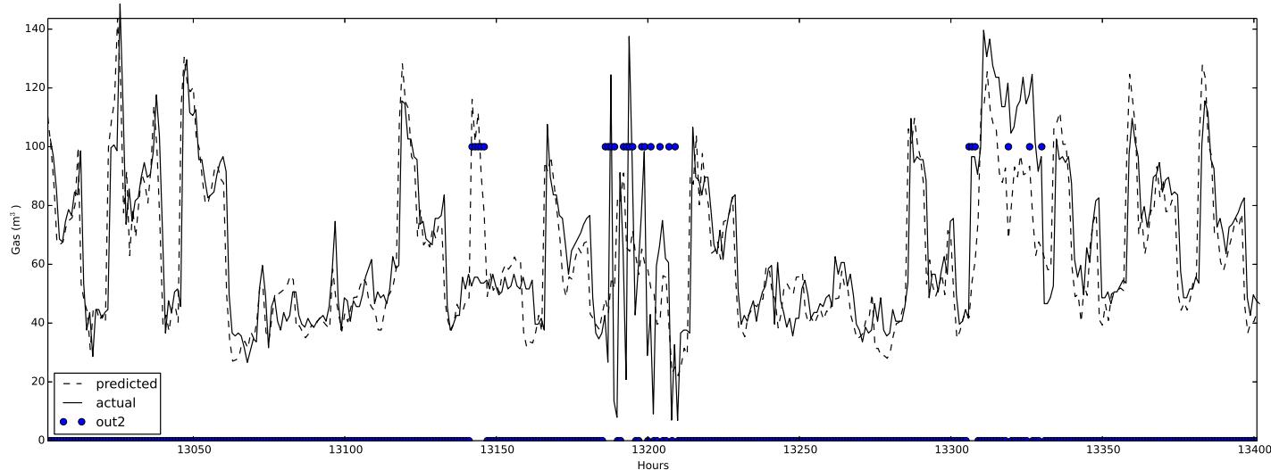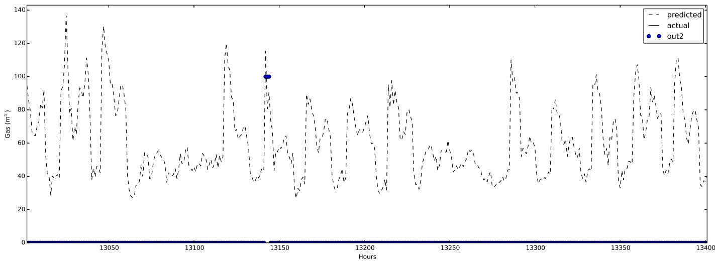Fig. 8: Outlier Detection with Synthetic Generated Data. The Circle Represents the Hours Where an Outlier is Detected Fig. 9: Outlier Detection Where A Sunday One Replaced the Gas Consumption of A Weekday. 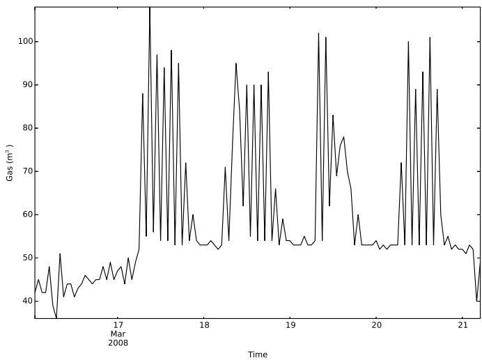The (Three) Circles Represent the Outliers Detected by the System  Fig. 10: Strange Zig-Zag Behaviour Found by the Algorithm Table III: Best Selected Results in Building 740-Nth, to Compare the Arima, ANN and Hybrid Model. Hymse is the Hybrid Model with MSE Cost Function, While Hymlse is the Same Model with MLSE Cost Function <table><tr><td>Model</td><td>neurons</td><td>epochs4</td><td>RMSE</td><td>MAPE</td><td>MAE</td></tr><tr><td>ARIMA5</td><td>-</td><td>-</td><td>88.50</td><td>117.27</td><td>22.52</td></tr><tr><td>ANN</td><td>80</td><td>15</td><td>11.95</td><td>34.78</td><td>8.52</td></tr><tr><td>HyMSE</td><td>80</td><td>70</td><td>9.4</td><td>27.66</td><td>6.90</td></tr><tr><td>HyMLSE</td><td>150</td><td>140</td><td>10.02</td><td>30.05</td><td>7.26</td></tr></table> Table IV: Best Selected Results for All the Buildings Table III: Best Selected Results in Building 740-Nth, to Compare the Arima, ANN and Hybrid Model. Hymse is the Hybrid Model with MSE Cost Function, While Hymlse is the Same Model with MLSE Cost Function <blockquote><table><tr><td>Model</td><td>neurons</td><td>epochs</td><td>RMSE</td><td>MAPE</td><td>MAE</td></tr><tr><td>740-NTH</td><td>150</td><td>140</td><td>10.02</td><td>30.05</td><td>7.26</td></tr><tr><td>761-KMH</td><td>150</td><td>140</td><td>2.49</td><td>18.30</td><td>1.00</td></tr></table></blockquote> An ANN with the standard cost function MSE was also trained, apparently resulting in a smaller RMSE error in a faster way (section V-B). Although this can be true, the Hybrid MLSE model was more precise and better at detecting possible outliers. They contributed the most to the error. <blockquote><table><tr><td>Model</td><td>neurons</td><td>epochs</td><td>RMSE</td><td>MAPE</td><td>MAE</td></tr><tr><td>740-NTH</td><td>150</td><td>140</td><td>10.02</td><td>30.05</td><td>7.26</td></tr><tr><td>761-KMH</td><td>150</td><td>140</td><td>2.49</td><td>18.30</td><td>1.00</td></tr></table></blockquote> An ANN with the standard cost function MSE was also trained, apparently resulting in a smaller RMSE error in a faster way (section V-B). Although this can be true, the Hybrid MLSE model was more precise and better at detecting possible outliers. They contributed the most to the error. An ANN with the standard cost function MSE was also trained, apparently resulting in a smaller RMSE error in a faster way (section V-B). Although this can be true, the Hybrid MLSE model was more precise and better at detecting possible outliers. They contributed the most to the error. In section V-B the results in the different buildings can be read. ## VI. FUTURE WORK ARIMA models can't detect more than one seasonality, but it can be helped with Fourier terms and ARIMA dummy variables to produce reasonable forecasts. When multi-seasonality is present, an algorithm like TBATS can overpass the ARIMA one and detect it. This non-parametric model described in [50] could be substituted for the ARIMA one as a feature of the ANN. At the moment, it is very slow, but it is very recent, so it will probably be improved. The daily pattern could be seen in the transformed Fourier space applying the Modified Discrete Cosine Transform (MDCT) [51]. In theory, this could help as well to understand the pattern, but it was only applied once by [52], with scarce results. ANNs are sensitive to missing values and irregularities, but it was not possible to contact the building managers in order to confirm/identify previously known outliers. For this reason the ANN training was done with not entirely perfect data, and this probably affected the performance. It is necessary to contact these building managers to further help with the training of this algorithm. The input variables were scaled, standardizing them to a midrange 0 and range $[-1,1]$. It is also possible to normalize them to have mean 0 and standard deviation 1. In this case, Robust estimates of location and scale are desirable if the inputs contain outliers. Some examples are [53] and the recent [54], which can be the basis of a future refinement of the ANN inputs. In future work, it is possible to break down the contrast between the MSE and the MLSE costs in the forecast and in the exception recognition. Before 2006, ANN was quite often connected with the Backpropagation calculation and with the 1-stowed away layer design. The issue with these designs is that they stall out in unfortunate neighborhood optima. In 2006, there was an enormous advancement principally began by [55], which is called Deep learning, and it addresses the new design of ANNs in light of multi-stowed away layers and new calculations. Future enhancements can be founded on Repetitive Brain Organizations (RNNs) and Limited Boltzmann Machines (RBMs), which were, as of late, ended up being fascinating in time-series gauging [52], [56], [57]. The Pylearn2 [44] RNN structure is being worked on. ## VII. CONCLUSION No model can treat all circumstances precisely for a lot of verifiable burden information. The unpredictable variance of the gas utilization was not really unsurprising, thus the ANN model was assisted with powerful expense capability and with the notable ARIMA model. Although different papers introduced comparative models to figure out electric utilization, the mixture model introduced here is practically interesting on the grounds that it centers around estimating momentary gas utilization, which is extremely sporadic and not effectively unsurprising with exemplary techniques. Since the indicator is exceptionally precise (with RMSE from $8m^3$ in building 740-NTH to RMSE 2.5 $m^3$ in building 761KMH), the anomaly component can undoubtedly distinguish weird ways of behaving characterizing an edge esteem in the certainty stretch without the need to have past instances of anomalies. The aim of this paper is to determine the profoundly sporadic gas utilization time series. Yet, it is accepted that comparable outcomes could likewise be acquired with the electric utilization time series. It is trusted that this could prompt another examination of the energy utilization in open structures.

Generating HTML Viewer...

References

57 Cites in Article
E Eurostat (2013). Energy balance sheets -2010-2011 -2013 edition.
(2009). European Parliament and Council of the European Union.
Nest (2014). Energy savings from nest white paper preview.
S Katipamula,M Brambley (2005). Review article: methods for fault detection, diagnostics, and prognostics for building systems-a review, part i.
Siyu Wu,Jian-Qiao Sun (2011). Cross-level fault detection and diagnosis of building HVAC systems.
Pedro González,Jesús Zamarreño (2005). Prediction of hourly energy consumption in buildings based on a feedback artificial neural network.
Alberto Neto,Flávio Fiorelli (2008). Comparison between detailed model simulation and artificial neural network for forecasting building energy consumption.
E D' Andrea,B Lazzerini,S Del Rosario (2012). Neural networkbased forecasting of energy consumption due to electric lighting in office buildings.
G Zhang (2003). Time series forecasting using a hybrid arima and neural network model.
M Khashei,M Bijari (2010). An artificial neural network (p, d, q) model for timeseries forecasting.
R Brown,I Matin (1995). Development of artificial neural network models to predict daily gas consumption.
A Khotanzad,H Elragal,T-L Lu (2000). Combination of artificial neural-network forecasters for prediction of natural gas consumption.
M Adya,F Collopy (1998). How e! ective are neural networks at forecasting and prediction? a review and evaluation.
A Douglas,A Breipohl,F Lee,R Adapa (1998). The impacts of temperature forecast uncertainty on Bayesian load forecasting.
D Ranaweera,G Karady,R Farmer (1996). Effect of probabilistic inputs on neural networkbased electric load forecasting.
M Mozer (2007). Neural net architectures for temporal sequence processing.
M Ohlsson,C Peterson,H Pi,T Rognvaldsson,B Soderberg (1994). Predicting system loads with artificial neural networksmethods and results from" the great energy predictor shootout.
Robert Dodier,Gregor Henze (2004). Statistical Analysis of Neural Networks as Applied to Building Energy Prediction.
Betul Ekici,U Aksoy (2009). Prediction of building energy consumption by using artificial neural networks.
R Cleveland,W Cleveland,J Mcrae,I Terpenning (1990). Stl: A seasonal-trend decomposition procedure based on loess.
G Zhang,B Patuwo,M Hu (1998). Forecasting with artificial neural networks:: The state of the art.
Rob Hyndman,Yeasmin Khandakar (2007). Automatic Time Series Forecasting: The<b>forecast</b>Package for<i>R</i>.
No ethics committee approval was required for this article type.
Data Availability
Not applicable for this article.
How to Cite This Article
Azizul Hakim Rafi. 2026. \u201cUse of Robust Artificial Neural Networks and ARIMA in Detecting Brief Anomalies in Gas Consumption\u201d. Global Journal of Computer Science and Technology - D: Neural & AI GJCST-D Volume 24 (GJCST Volume 24 Issue D2): .
Explore published articles in an immersive Augmented Reality environment. Our platform converts research papers into interactive 3D books, allowing readers to view and interact with content using AR and VR compatible devices.
Your published article is automatically converted into a realistic 3D book. Flip through pages and read research papers in a more engaging and interactive format.
This paper introduces an innovative system for outlier detection that combines the strengths of an Auto-regressive Integrated Moving Average (ARIMA) model and an Artificial Neural Network (ANN). While ARIMA is traditionally used for linear predictions and ANNs for nonlinear forecasting, this study demonstrates their synergistic capabilities in capturing complex, non-linear relationships between meteorological forecast variables and gas consumption patterns. The resulting system can identify anomalies, aiding building managers in reducing energy waste in HVAC systems. The process comprises two phases: first, it predicts short-term gas consumption patterns using historical data, and then it identifies outliers by detecting deviations from expected values. Remarkably, this outlier detection process doesn’t require predefined labeled examples, thanks to the system’s highly accurate gas consumption forecasts, characterized by a root mean square error (RMSE) ranging from 8 m3 to 2.5 m3.
Our website is actively being updated, and changes may occur frequently. Please clear your browser cache if needed. For feedback or error reporting, please email [email protected]
Thank you for connecting with us. We will respond to you shortly.