I. INTRODUCTION

Internal combustion Engines (ICE) play a crucial role in modern transportation and industry, being employed in diverse sectors like planes, cars, and power generation [1-3]. The ever-strict regulations on pollutant emissions of harmful gases (NOx, CO, HC and soot) and ${\mathrm{CO}}_2$ are forcing the ICE to become more efficient to reduce their impact on the environment [4, 5]. Therefore, the research field is called to make significant efforts to enhance the overall efficiency of ICEs [6, 7]. In the industry, achieving a $0.05\mathrm{\%}$ improvement in efficiency is a challenging and exceptional endeavor, directly impacting both fuel consumption and emissions. The provided Table exemplifies this; for instance, NOx emissions decrease from 0.08 to $0.06\mathrm{g}/\mathrm{km}$. Even minor differences between Euro standards require substantial efforts, motivating advanced research.

	Starting from	CO2(g/km)	HC (g/km)	NOx (g/km)	HC + NOx (g/km)	PM (g/km)
Euro 1	12/1992	2.72	/	/	0.97	/
Euro 2	01/1997	2.30	/	/	0.5	/
Euro 3	01/2000	2.20	0.20	0.15	/	/
Euro 4	01/2005	1.00	0.10	0.08	/	/
Euro 5	09/2009	1.00	0.10	0.06	/	0.005
Euro 6	08/2014	1.00	0.10	0.06	/	0.005

Original Equipment Manufacturers (OEMs) and the engine research community agree in considering an engine thermal efficiency, of the Spark - Ignition (SI) engines, above $40\mathrm{\%}$ as a feasible goal [8, 9]. Advanced combustion techniques such as cooled external exhaust gas recirculation (EGR) [10], engine boosting in conjunction with downsizing [11], water injection [12], and lean mixture operations [13- 15] proved to be effective ways to meet these demands. EGR reduces combustion temperatures, mitigating NOx emissions while improving efficiency by reducing pumping losses and improving combustion stability. Combining boosting with downsizing results in smaller engines that maintain or even enhance power output. This reduces fuel consumption and emissions due to the smaller engine size. Water injection improves efficiency by cooling the intake charge, reducing knock, and allowing for higher compression ratios. It also reduces emissions by lowering combustion temperatures. Operating with a lean air-to-fuel mixture reduces fuel consumption and ${\mathrm{CO}}_2$ emissions. It can, however, increase NOx emissions, which is where technologies like EGR and water injection can offset these drawbacks. However, the implementation of new technologies increases the engine complexity and magnifies the amount of data to be collected from the different physical sensors both during engine calibration and run-time operations [16]. As a result, significant computational efforts are required, resulting in longer operating times and increased costs [17]. Advanced technologies, such as the Machine Learning (ML) approach [18], are currently being investigated to effectively monitor the vehicle's parameters of spark ignition (SI) engine with the aim of overcoming the abovementioned issues. The optimization of the engine design passes through effective efficiency, whose knowledge can be of pivotal importance to improve the engine's performance while reducing fuel consumption and pollutant emissions, at the same time.

Incorporating insights from advanced technologies like Machine Learning, the optimization of engine design can be further refined, leveraging data-driven approaches to enhance combustion strategies and ultimately achieve greater efficiency and emission reduction. Efficient performance can be assessed by measuring the engine's delivered torque and fuel consumption. However, implementing these measurements directly on-board is challenging using physical instruments. Preliminary characterizations on specific test benches are required to calibrate the engine properly [19]. In the present study, an unconventional methodology, primarily leveraging a NARX ML model, is being introduced to forecast engine parameters that would typically pose significant challenges for experimental measurement. This model is intended to function as a virtual sensor for quantities not typically available in today's commercial vehicles. Extending this concept, this approach might potentially substitute the measurement of certain parameters currently ascertained using conventional sensors and actuators, thereby resulting in cost reduction.

In a study conducted by Togun and Baysec [20], they used an artificial neural network (ANN) to predict the specific fuel consumption (SFC) and torque of a gasoline engine. The input parameters considered were ignition advance, throttling status, and engine speed, while the outputs were predicted separately using different network architectures. To predict engine torque, a network architecture consisting of 3 input parameters, one hidden layer with 13 neurons, and one output layer was used. For predicting brake-specific fuel consumption (BSFC), a 3-15-1 network architecture was used. The results for torque prediction showed correlation coefficients of approximately 0.99 for both training and testing. For BSFC prediction, the correlation coefficients were 0.9971 for training and 0.98331 for testing. The mean absolute percentage error (MAPE) for torque measurement was 0.2912 for training and 1.74 for testing. As for BSFC prediction, the MAPE values were 1.0186 for training and 2.7588 for testing. Cay [21] developed three separate artificial neural network (ANN) models to predict brake-specific fuel consumption (BSFC), exhaust gas temperature (EGT), and effective power. They wanted to study the impact of three input parameters on these output parameters. The inputs to the ANN included fuel flow, speed, inlet manifold temperature, torque, and water temperature. During testing, the mean error percentage was found to be less than $2.7\mathrm{\%}$, and root mean square error (RMSE) values were less than 0.02, indicating the accuracy of the predictions. For both training and testing data, the ${\mathsf{R}}^2$ value, which represents the goodness of fit, was close to 0.99, further demonstrating the effectiveness of the ANN models. Golcu et al. [22] investigated how variable valve timing affects the performance and fuel economy of an engine. They experimented by changing the crank angle by 10 to 30 degrees and created an artificial neural network (ANN) model using valve-timing and speed as inputs. The output data chosen were fuel flow and torque. The testing results for torque and fuel flow showed root mean square errors (RMSE) of approximately $0.9\mathrm{\%}$ and $0.28\mathrm{\%}$, respectively. All the mentioned references used the Back Propagation (BA) approach for the forecasting activities.

A previous work of the same research group [23], showed the performance of a NARX (nonlinear autoregressive network with exogenous inputs) structure in reproducing with remarkable accuracy across various transient cycles the torque delivered by a SI engine. The optimized NARX architecture exhibited an average error up to $70\mathrm{\%}$ less than a critical threshold of $10\mathrm{\%}$.

and operational working time. Hyper parametric optimizations of the tested architectures, i.e. BP and NARX, were realized through the grid search method based on a transient cycle experimentally realized. The results show that BP reproduces physical trends well with an average error of $5.9\mathrm{\%}$ for torque and $4.7\mathrm{\%}$ for fuel consumption, both below a critical threshold of $10\mathrm{\%}$. NARX outperforms BP by $35\mathrm{\%}$ in both cases, with a lower average error under $4\mathrm{\%}$ for torque and fuel consumption.

II. MATERIALS AND METHODS

a) Experimental Setup

Tests were performed on a 1L three-cylinder turbocharged engine of $62\mathrm{kW}$, chosen to represent a common and efficient configuration in modern automobiles and in all test benches, enabling a realistic and relevant assessment of engine parameters for widespread applicability and industry relevance. The engine operates in Port Fuel Injection (PFI) with European market gasoline, and it is controlled by an electric motor both in motored and firing conditions.

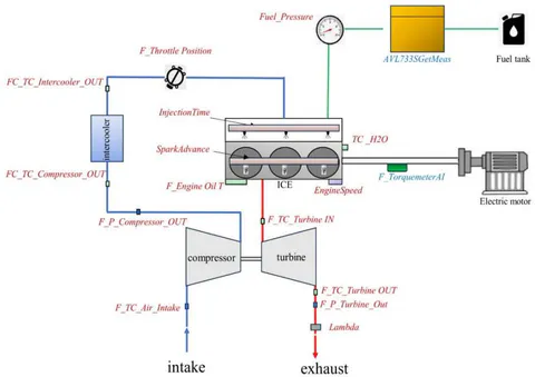
More detailed information about the engine and experimental setup can be found in [23]. The torque delivered by the engine is measured using a torque meter located near the engine crankshaft whereas the fuel consumption is computed by a dynamic AVL 733Sfuel meter. An AdaMo Hyper software records all parameters during engine operations, enabling the simultaneous control of engine speed, torque, and valve throttle position. AdaMo acquired data from various sources, including the Engine Control Unit (ECU), pressure sensors, thermocouples, torque meter, and dynamic fuel meter, at a sampling frequency of $10\mathrm{Hz}$. From this data, a total of 15 variables, that were deemed most characteristic, were selected as inputs (red in Figure 1) for the neural structure to predict torque and fuel consumption (blue in Figure 1). The signals coming from thermocouples TCK and pressure sensors PTX 1000 are acquired by data acquisition systems of National Instrument. All the above quantities are recorded by the AdaMo Hyper software during engine operations. Table 2 displays some values of the variables acquired during the experimental activities.

Parameter	Unit	Handled by
F_TorquemeterAI	Nm	TorqueMeter
AVL7335GetMeas	kg/h	Dynamic Fuel Meter 733S
EngineSpeed	rpm	ECU
F_Throttle Position	%	ECU
InjectionTime	us	ECU
Fuel_Pressure	bar	ECU
SparkAdvance	CAD bTDC	ECU
TC_H2O	°C	ECU
F_Engine Oil T	°C	PT100 sensor
F_TC_Turbine IN	°C	Thermocouple TCK
F_TC_Turbine OUT	°C	Thermocouple TCK
F_TC_Air_Intake	°C	Thermocouple TCK
FC_TC_Intecooler_OUT	°C	Thermocouple TCK
FC_TC_Compressor_OUT	°C	Thermocouple TCK
F_P_Compressor_OUT	mbar	PTX1000 sensor
F_P_Turbine_Out	°C	Thermocouple TCK
Lambda	-	Lamba Sensor

Timestamp	s	0.1	0.2	......	200	200.1	......	349.9	350	......	525.3	525.4
F_TorquemeterAI	Nm	14.9	14.9	......	4.8	5.3	......	7.2	6.3	......	6.8	6.3
AVL733SGetMeas	kg/h	1.908	1.827	......	0.587	0.57	......	0.945	0.945	......	0.25	0.511
EngineSpeed	rpm	1201	1201	......	1369	1361	......	2311	2348	......	2403	2439
F_Throttle Position	%	8.2	8.2	......	6.6	6.2	......	10.9	11.7	......	10.2	10.2
F_Engine Oil T	°C	57.2	57.2	......	60.1	60.7	......	63.2	63.2	......	65.8	65.8
F_TC_Turbine IN	°C	151.9	179.2	......	476.3	476.3	......	559.6	559.6	......	567.9	567.9
F_TC_Turbine OUT	°C	112.5	112.5	......	295	295	......	387.6	388.1	......	402.9	402.9
F_TC_Air_Intake	°C	34.2	34.2	......	35.9	35.9	......	36.2	36.2	......	35.9	35.9
FC_TC_Intercooler_OUT	°C	33.8	33.8	......	34.9	34.9	......	35.9	35.9	......	35.6	35.6
F_TC_Compressor_OUT	°C	12.01	12.01	......	10.13	10.13	......	11.12	11.12	......	14.09	14.09
F_P_Compressor_OUT	mbar	987	987	......	985.1	985.1	......	986.1	986.1	......	989.1	989.1
F_P_Turbine_Out	mbar	982.29	982.29	......	982.83	982.83	......	983.22	983.22	......	981.69	981.69
Fuel_Pressure	bar	3215	3215	......	3215	3215	......	3204	3204	......	3215	3215
InjectionTime	us	3404	3404	......	2361	2440	......	2361	2361	......	2167	2010
SparkAdvance	CAD	24.5	24.5	......	26.75	27	......	32.5	32.5	......	32.75	32.75
TC_H2O	°C	49.4	49.4	......	46.9	46.9	......	49.4	49.4	......	50.6	50.6
Lambda	-	1.008	1.008	......	0.969	0.938	......	0.945	0.945	......	0.883	0.898

b) Data Correlation Analysis

Starting from the initial dataset, it is important to understand the relationship between the numerous input parameters recorded during the experimental activities and their impact on the engine-delivered torque and fuel consumption.

It is essential to evaluate each parameter individually to understand the influence of such parameters on the output prediction to identify if they can be removed in order to reduce the model's complexity by improving its accuracy at the same time.

It is worth mentioning that the variables for which you want to assess the correlation should be sortable and, ideally, continuous. To this aim, three different correlation parameters have been employed: Pearson correlation coefficient R [24], Spearman correlation coefficient $\rho$ [25] and Shapley value $\phi$ [26].

The Pearson correlation coefficient $R$ evaluates the degree of linear correlation between parameters by assessing the direction and strength of their relationship based on their actual values, as follows (eq.1):

where $n$ is the number of input parameters $x_i,y_i$ the variable to be predicted, CoV(X,Y) is the covariance of two sets of data $X$ and $Y$, and ${\sigma }_x$ and ${\sigma }_y$ the standard deviations of such sets. The Pearson correlation coefficient also ranges from -1 to +1. A positive value indicates a positive linear relationship, while a negative value indicates a negative linear relationship. A coefficient close to 0 means there is little to no linear relationship between the variables.

The Spearman correlation coefficient $\rho$ is a statistical method used to determine the strength and direction of the relationship between two variables. It is a non-parametric measure, meaning it doesn't assume a specific distribution for the data. Instead, it focuses on assessing the monotonic relationship between the variables. Monotonicity implies that as one variable increases, the other variable consistently either increases or decreases, though not necessarily at a constant rate. The Spearman correlation (eq. 2) evaluates the similarity of the rank orders of data points, disregarding their actual numerical values.

where $d_i^2$ is the rank difference of two variables after sorting. The Spearman correlation coefficient ranges from -1 to +1. A positive value indicates a direct (increasing) monotonic relationship, while a negative value indicates an inverse (decreasing) monotonic relationship. A coefficient of 0 means there is no monotonic relationship between the variables and indicates a weaker correlation and a smaller influence relationship.

The Shapley value $\phi$ [26](eq. 3) attempts to explain an instance's prediction by assessing the contribution of each attribute to the forecast. The Shapley Value calculates the average contribution of each player across all possible coalitions to quantify the impact of the single measured quantities on the objective function.

where ${\phi }_i$ is the Shapley value for player $i$, $\nu (S)$ is the worth coalition $S$, $n$ is the number of total players and $m$ is the number of players in the coalition $S$ before player $i$ joins $(0\le m\le n-1)$. Positive values imply a positive correlation between input and target while negative values imply that the player detracts from the coalition's value when they join. It is worth highlighting that, as dealing with two output variables, two separate sensitivity analyses were conducted, one for torque and one for fuel consumption. This allowed to identify how the input variables can independently influence the outputs.

To explain the choice of the input parameters used to build the tested neural structures, a step-by-step explanation is reported below. Table 3 shows positive and negative values to highlight the trend correlation between input and output. To quantify the influence, the absolute value (ABS) of such quantity must be taken into account.

Since the goal of the study is to build a single ANN capable of simultaneously predicting both variables under examination, some considerations were made regarding the indicators, in order to include all influential variables while avoiding the exclusion of others that might positively impact one of the two outputs. First, all variables that simultaneously exhibit negative Shapley values have been removed from the input dataset, i.e., SparkAdvance, F_P_Turbine_Out, FC_TC_Air_Intake,Lambda, F_TC_Turbine_OUT,FC_TC_Compressor_OUT. Even if Fuel_pressure positively influences the FC prediction, the high negative value showed for the torque forecasting led to excluding it as well. $F\mathrm{\_}EngineOilT$ presents a shapley close to zero for one output and negative for the other: therefore, also sucha variable has been excluded from the initial dataset. Engine Speed was included in the initial dataset because, despite the negative Shapley value for torque, the Spearman and Pearson correlations of both output variables with Engine Speed were among the highest values.

In other words, 8 of the initial 15 variables have been excluded resulting in roughly over $50\mathrm{\%}$ of the initial input variables.

Variable Name	Unit	Torque (F_TorqueMeterAI)			Fuel Consumption (AVL733SGetMeas)
		Shapley	Spearman	Pearson	Shapley	Spearman	Pearson
FC_TC_Compressor_OUT	°C	-8.40	0.55	0.53	-2.56	0.82	0.83
EngineSpeed	rpm	-0.20	0.59	0.58	0.05	0.82	0.73
F_Throttle Position	%	1.03	0.81	0.83	0.01	0.84	0.79
F_Engine Oil T	°C	0.19	-0.01	-0.09	-0.13	-0.17	-0.19
F_TC_Turbine IN	°C	2.19	0.42	0.35	0.03	0.53	0.43
F_TC_Turbine OUT	°C	-1.95	0.36	0.26	-0.08	0.43	0.37
F_TC_Air_Intake	°C	-9.95	-0.11	-0.14	-1.50	-0.27	-0.24
FC_TC_Intercooler_OUT	°C	16.37	0.19	0.12	0.73	0.13	0.14
F_P_Compressor_OUT	mbar	55.37	0.55	0.53	61.43	0.82	0.83
F_P_Turbine_Out	mbar	-54.43	0.12	0.06	24.40	0.06	0.09
FuelPressure	bar	-7.49	-0.40	-0.41	1.17	-0.35	-0.33
InjectionTime	μs	0.96	0.62	0.64	0.04	0.22	0.35
SparkAdvance	CAD	-0.62	0.43	0.40	-0.02	0.70	0.55
TC_H2O	°C	4.22	0.18	0.10	0.11	0.10	0.09
Lambda	-	-1.00	-0.20	-0.34	-0.01	-0.32	-0.37

Since, previous work of the same research group [27] certified increments in the prediction performance when operating with a reduced dataset, the artificial architectures presented have been built by considering a total of 7 input variables. As mentioned before, by reducing the number of input variables, the model becomes more compact, requiring less storage space and this leads to faster training times, quicker model convergence, and shorter inference times during predictions.

c) Preparing the Initial Dataset

After conducting the initial analysis to identify the relevant input parameters, the data (Table 3) is normalized to reduce potential prediction errors and enable the model to converge more quickly.

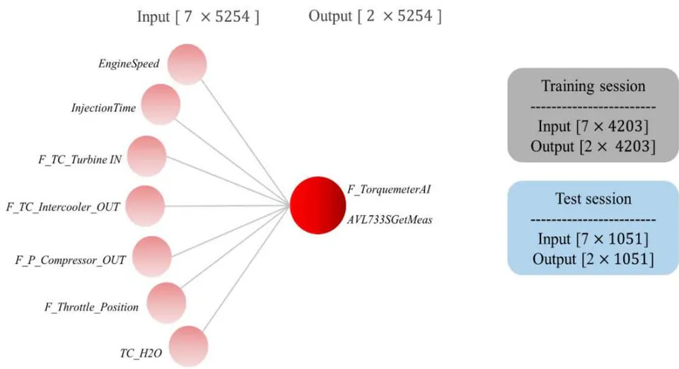
Normalization is necessary to handle variations in input and output parameters effectively. During normalization, the values are scaled to fit within the range [0, 1]. Once the prediction process is complete, the predicted data is de-normalized to facilitate a direct comparison with the actual target values obtained from experimental measurements. Figure 2 illustrates the complete dataset used in this study, including the separation of input and output. The training session was realized on $80\mathrm{\%}$ of the entire dataset, while the test session, concerning the prediction was realized on the remaining $20\mathrm{\%}$. It is worth reminding that AdaMo acquires data with a sampling frequency of $10\mathrm{Hz}$, therefore 5254samples correspond to 525.4 seconds.

III. CONSTRUCTION OF THE NEURAL ARCHITECTURES

This section details the design and refinement of neural network architectures to predict SI engine torque and fuel consumption. It includes considerations for optimal structure, training techniques like Back Propagation and the NARX approach, and evaluation metrics for performance assessment.

a) Preliminary Considerations

This section describes the different neural network architectures employed in this study to predict the torque delivered and fuel consumption of the SI engine (see 2.1 Experimental setup) and all the operations the authors made to optimize the internal structure of each of them. In the process of optimization, dealing with numerous variables can be quite challenging. To address this issue, certain considerations must be made to streamline the task. By incorporating these considerations [28-30]:

• The number of neurons $N$ in each hidden layer should be between the number of inputs and the number of outputs (i.e., ).
• The number of neurons in each hidden layer should be $2/3$ the number of inputs, plus the number of outputs (i.e., $N=6$ ).
• The number of neurons in each hidden layer should be less than twice the number of inputs (i.e., ).

The optimization process can be more efficient. A maximum of 4 hidden units, equal to the double number of variables to be predicted, has been chosen. Each hidden layer is composed of diverse numbers of neurons, i.e. from 4 to 13, by following the considerations listed. The number of the epoch was set equal to 1000, since this value has been observed to achieve good performance with reduced computational efforts. To avoid over fitting issues, Early Stopping technique [31] is also employed to stop the training process if no significant improvement in performance (MSE eq.4) is recorded above a certain number of epochs. The initial learning rate is set to 0.0001 and the bias and weights of each neuron are continuously optimized by Adaptive Moment Estimation (Adam) which combines the benefits of both RMSprop and momentum optimization to automatically adjusts the learning rate, based on historical gradients and past updates [32]. In fact, it is worth highlighting that, if the learning rate is too high, the model can become unstable and therefore unable to find the best solution. On the other hand, if the learning rate is too small, the model may take a long time to learn without finding a good solution. So, finding the right learning rate is important to train the model effectively [33]. To sum up:

• The number of neurons varies from 4 to 13.
• The hidden layers vary from 1 to 4.
• The number of the epoch is set to 1000.
• The initial learning rate is set at 0.0001.

The definition of the optimal neural structures is determined through preliminary analysis considering the training sessions' performance. To evaluate the training performance of model parameters, the loss function is created, and the mean square error (MSE) is chosen as the loss function (eq.4):

with $n$ the number of samples. Set the number of network epoch iterations to 1000, to calculate the final value of the loss function for each prediction model once the network training reaches the maximum learning iteration.

To make a comparison over the entire predicted range, for each forecast $i$, the deviation of the prediction

$Y_{predicted}^i$ from the target $Y_{target}^i$ throughout the range is computed (eq.5):

where $N$ is the number of samples considered for the test case and $i$ the $i^{th}$ sample. The average percentual error, i.e. $Er{r}_{avg}$, is computed as well to draw attention to the global prediction quality. For this kind of application, a maximum critical threshold of 10 is established for the abovementioned errors. Moreover, other two evaluation metrics are used to compare the test performance of the architectures, i.e. RMSE (eq.6) and $R^2$ (eq.7).

where $Y_{avg}^i$ is the average value of the prediction.

Due to the large number of combinations analyzed for each structure, it is not feasible to illustrate the performance of every single one. As a result, the authors focused on presenting the features of the best-performing structure for each ANN.

b) Back Propagation

The BP structure has been optimized through the grid search method by testing the following hyper parameter combinations:

• One input layer with size equals the number of features in the input data.

• From 1 to 4 hidden layers $H_L$ each of which with 4 to 13 neurons $N$. After each hidden layer, a fully connected layer is applied, followed by a ReLU activation function [35].

• An output layer with two output units for the two target variables which directly provides the predicted values without any further processing.

• A regression layer computes the mean squared error (MSE) loss between the predicted output and the target output during the training process.

• The training process presents an Adam optimizer, as previously mentioned, a maximum of 1000 epochs, and the data is processed in mini-batches $M_b$ of 8, 16, 32, 64 or 128 samples per iteration.

c) NARX

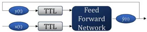
NARX approach is a type of recurrent dynamic neural network employed for modeling nonlinear dynamic systems and time-series forecasting [36]. The NARX network can have either a series-parallel (i.e., open-loop) or a parallel architecture (i.e., close-loop) [37], as illustrated in Figure 3.

(a)

(b) Figure 3: Design of the Type of NARX Architectures: (A) Open-Loop Configuration and (B) Close-Loop One In the series-parallel architecture (Figure 3 (a)), the network predicts the desired output value, denoted as $\hat{y}(t)$, based on the current and past values of the input $x(t)$ and the actual past value of the time series, $y(t)$ (eq.8).

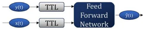
with $n_x\in n_y$ input memory order and output memory order, respectively.

On the other hand, in the parallel architecture (Figure 3 (b)), the prediction relies on the current and past values of $x(t)$ and the predicted value of $\hat{y}$ (t) (eq.9).

During the training phase, a series-parallel architecture is utilized because it has access to the true past value of the time series. Subsequently, this architecture is transformed into a parallel one, which is more suitable for multi-step-ahead forecasting.

The NARX structure has been optimized through the grid search method by testing the following hyper parameter combinations.

• From 1 to 4 hidden layers $H_L$ each of which with 4 to 13 neurons $N$.
• An output layer with two output units for the two target variables which directly provides the predicted values without any further processing.
• A regression layer computes the mean squared error (MSE) loss between the predicted output and the target output during the training process.
• The training process presents an Adam optimizer, as previously mentioned, and a maximum of 1000 epochs.

IV. RESULTS AND DISCUSSIONS

a) Results on Training

The first comparison between the proposed algorithms is performed via training_loss function as described in the previous paragraph. The structure of the architectures presenting the best performance on training are composed as follows.

• Back Propagation is composed of three hidden layers $H_L$, respectively with 11, 9, and 9 neurons $N$, mini-batch size $M_b$ equals 128, and learning rate equals 0.01.
• NARX is composed of two hidden layers $H_L$, respectively with 4 and 9 neurons $N$ (Figure 4). Also, the sum of neurons of the two hidden layers (i.e. 13) does not exceed twice the number of inputs (see the previous considerations listed regarding the definition of the number of neurons.

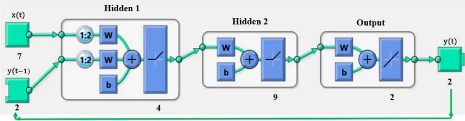
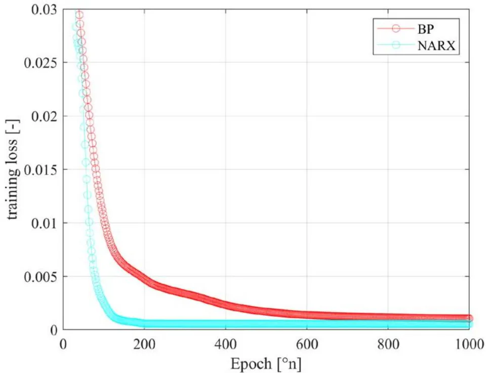
Figure 5 illustrates a comparison of the training loss among the different architectures. In all cases, there is a consistent decreasing trend in training loss as the number of epochs increases. These architectures tend to reach a point of stability around 600 epochs, where the training loss falls below 0.001 by the time the ${1000}^{\text{th}}$ epoch is reached. This indicates that the models converge effectively without experiencing over fitting issues. Notably, the NARX architecture demonstrates the quickest convergence, achieving a training loss below 0.005 in approximately at 100 epochs. Furthermore, once it reaches this stabilized state, it exhibits minimal oscillations in the training loss, suggesting that it may be more robust compared to the other architectures.

b) Results on Test

Starting from the Back Propagation, Figure 6 displays the comparison between the experimental traces experimentally obtained (black color) and the ones predicted by the optimized BP structure (red color). The prediction error distribution generated by the BP architecture is also presented to enhance the assessment of forecasting accuracy. This approach aims to provide a more precise evaluation of the predictive performance in quantitative terms. From a qualitative point of view, BP is capable of reproducing the physical trend of both analyzed targets. In particular, it well-reproduces the fluctuation of the FC signal, which is characterized by lower oscillations if compared to the torque signal. It is worth noting that, BP model reproduces greater signal fluctuation, particularly noticeable from 465 seconds to 495, taking the torque signal as an example. However, it underestimates the highest peak around 490 seconds. The architecture performs an average error ${\mathrm{Err}}_{\mathrm{avg}}$ of about $5.9\mathrm{\%}$ regarding the torque prediction and of about $4.7\mathrm{\%}$ on the fuel consumption, both less than the critical threshold of 10. Concerning the torque prediction, the architecture exceeds 169 times the $\mathrm{Err}=10\mathrm{\%}$, corresponding to about $16\mathrm{\%}$ of the total samples predicted while, for the fuel consumption, it is able to enhance the prediction quality. In fact, even if the number of samples predicted over the $10\mathrm{\%}$ threshold is equal to 213, the structure is capable of well-reproducing the target trend. However, the maximum error computed in the FC prediction is $28\mathrm{\%}$, corresponding to about $0.025\mathrm{kg}/\mathrm{h}$ in the initial part of the test (around 420 seconds), and therefore negligible.

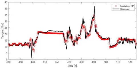
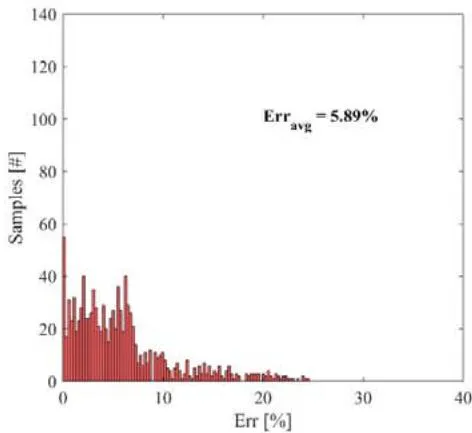
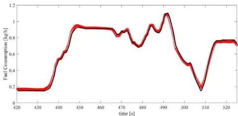
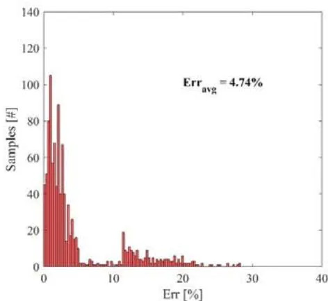
Figure 7 illustrates the outcomes of the NARX architecture, following the same format as Figure 6 did for the BP architecture. From a qualitative point of view, such a structure is able to mitigate the error in the prediction of BP where the experimental signals are approximatively constants, i.e. in the range from 142 to 152 seconds, and conversely to BP, is capable of reproducing the three highest torque peaks in the interval $450\mathbf{\nabla }\mathbf{\cdot }500$ seconds. NARX outperforms BP with ${\mathrm{Err}}_{\mathrm{avg}}$ respectively with about $3.8\mathrm{\%}$ and $3.1\mathrm{\%}$ of ${\mathrm{Err}}_{\mathrm{avg}}$ in torque and fuel consumption prediction, corresponding to improvements of about $35\mathrm{\%}$ in both cases. It shows only $6\mathrm{\%}$ of the predicted samples exceeding the $10\mathrm{\%}$ of Err, in the torque and FC predictions. In the latter case, the Err on prediction never exceeds $16\mathrm{\%}$, conversely to BP which shows errors up to $28\mathrm{\%}$.

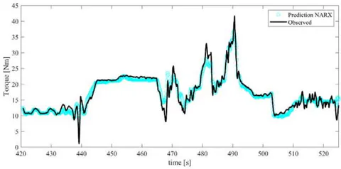
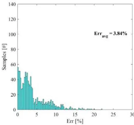
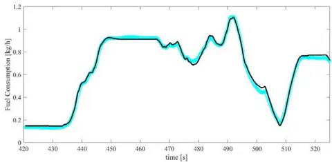
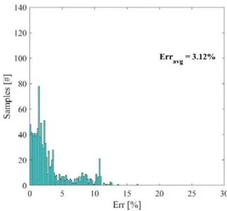
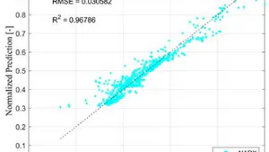
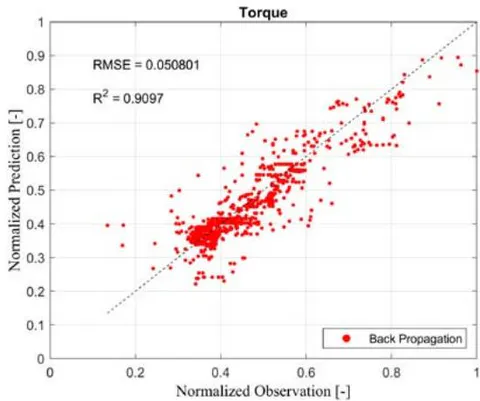
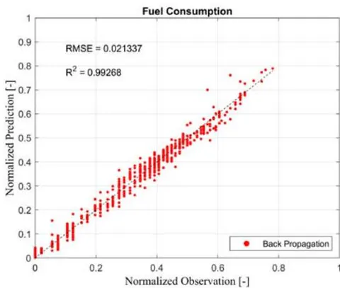
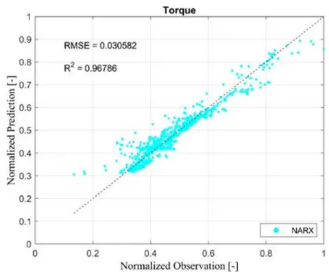
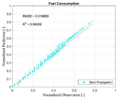
Figure 8 illustrates the regression accuracy of each model, as defined by eq.7, along with the corresponding Root Mean Square Error. Concerning the Torque Prediction, the NARX model stands out with superior accuracy and smaller prediction errors, as previously demonstrated. In contrast, the BP structure exhibits deviations in the lowest and highest ranges tested. Specifically, it tends to overestimate predictions for low values and underestimate them for high torque levels. NARX improves BP's R-squared values of about $6\mathrm{\%}$, and significantly reduces RMSE of about a $40\mathrm{\%}$.

These improvements mitigate the error associated with BP in all the analyzed range. Concerning the fuel consumption, the $R^2$ and RMSE certify again the capability of both structures to well-predicted such an output feature. Bot structures show R2 close to the unit and RMSE approximately equals to 0.02. These results confirm the higher ability of NARX to effectively addresses prediction of the analyzed targets and its superior nonlinear fitting capabilities.

Figure 8: Comparison between the Predictions Performed by the Tested Structures in Terms of $R^2$ and RMSE

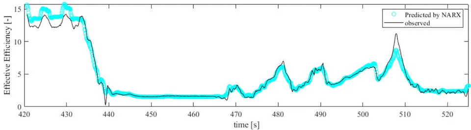
Based on the obtained results, from the torque and FC signals, it's possible to calculate the effective efficiency ${\mathfrak{H}}_{\mathrm{eff}}$ of the engineby usingeq.10, and then compare it with the experimental efficiency.

with Torque expressed in Nm, w the engine speed in rad/s, FC the fuel consumption in kg/s and Lower Heating Value (LHV) of the gasoline equals 44 MJ/kg. Figure 9reports the preliminary attempt to compare the efficiency computed from the signals experimentally obtained and the ones predicted by the optimized NARX structure and certifies effectiveness in accurately estimating efficiency across transient conditions.

V. CONCLUSIONS

The goal of this study was to develop an Al-based methodology for evaluating the overall efficiency of a three-cylinder SI engine by simultaneously predicting its torque and fuel consumption. It compared the performance of a Back Propagation (BP) structure with a Nonlinear Autoregressive Network with Exogenous Inputs (NARX) algorithm. In an effort to optimize prediction accuracy, a sensitivity analysis was conducted to select influential parameters while reducing computational complexity and operational time. The experimental dataset was acquired through transient cycle experiments, and hyper parameter optimizations were performed for both BP and NARX architectures using a grid search method.

The results clearly demonstrated that.

• All models effectively converged without over fitting, with training loss consistently decreasing as epochs increase. Notably, the NARX architecture exhibited the quickest convergence, reaching a training loss below 0.005 in around 100 epochs. This suggests its potential robustness if compared to BP.

• NARX outperformed BP in the test phases with an average error of about $3.8\mathrm{\%}$ for torque prediction and $3.1\mathrm{\%}$ for fuel consumption, representing a $35\mathrm{\%}$ improvement in both cases. The NARX model had fewer samples exceeding the $10\mathrm{\%}$ error threshold compared to BP.

• NARX demonstrated superior accuracy and smaller prediction errors in torque prediction compared to BP.BP exhibited deviations in the lowest and highest ranges, overestimating for low values and underestimating for high torque levels. NARX improved BP's $R^2$ values by approximately $6\mathrm{\%}$ and significantly reduced RMSE by about $40\mathrm{\%}$, mitigating errors across all analyzed ranges. Both models performed well in fuel consumption prediction, with high R-squared values close to the unit and low RMSE.

In summary, the NARX model consistently outperformed the BP architecture in terms of accuracy, prediction error, and robustness, particularly in torque prediction and efficiency estimation. Its ability to capture complex patterns and adapt to changing conditions underscores its superiority in nonlinear fitting. These compelling results underscore the NARX model's critical role in revolutionizing automotive design by significantly enhancing engine efficiency assessment. The model's remarkable predictive accuracy and adaptability hold immense promise for fostering innovation in the automotive industry, ultimately driving the development of greener and more sustainable automotive technologies. The NARX model stands as a valuable tool for engineers and researchers seeking to optimize internal combustion engines, shaping a future where energy-efficient and environmentally friendly vehicles play a central role in transportation.