## I. INTRODUCTION The dynamics of a planar two-link rigid robot having two revolute joints is non-linear and involves coupling between joint variables. Linear control is difficult to apply to such systems. In order to apply linear control theory for joint motion control of robots, a high gear ratio is used so that a linear PD or PID controller may be used. A computed-torque controller is a better controller than a linear PD or PID controller. It is a special application of 'feedback linearization' of nonlinear systems and computed-torque like controls appear in robust control, adaptive control etc. [1]. The motion of the joints of a robot can be controlled either by the approach of 'independent joint control' or by the approach of 'multivariable control' [2]. In 'independent joint control,' each joint of a robot is controlled as a single input/single-output (SISO) system. The coupling effects due to the motion of other links are treated as disturbances. On the other hand, the multivariable control facilitates the design of robust [3] and adaptive [4] nonlinear controllers that guarantee more stability and better tracking of arbitrary trajectories. Harris and Wang [5] have proposed mathematical models for the stabilization of closed-loop constrained robots. Slotine and Yang [6] have presented a computationally efficient time-optimal path-following algorithm for robots under actuator constraints. Few authors have made use of the concept of decoupled and invariant dynamics of manipulators during the design stage for achieving high-speed trajectory control of direct-drive manipulators [7] and the concept of dynamic isotropy for decoupling of inertia matrix for obtaining robust control [8]. A number of research works including Piazzi and Visioli [9], Constantinescu and Croft [10], Gasparetto and Zanotto [11] and Marcello et al. [12] have focused on formulating algorithms based on minimization of an objective function that helps in finding the time-optimal trajectories for the robots. Xavier et al. [13] have described how to build autonomous robots that can perform service tasks safely within the vicinity of humans. Machado et al. [14] have suggested that although direct design algorithm and computed torque controllers are superior to linear controllers, classical design approach can be implemented practically. This approach can be used to analyze and develop nonlinear model-based controllers for robots. Shiller and Chang [15] have proposed a method that helps in the reduction of tracking errors for high-speed articulated robots. This is achieved by preshaping the actual trajectory of the robot by using inverse control gains. Gradient search method is used to find the optimized control parameters for trajectory preshaping. Karger et al. [16] have proposed a hyperbolic trajectory for any degrees of freedom robot. The advantage of this trajectory is that it can be planned both in Joint space and Cartesian space with the requirement of inverse kinematics only at the initial and final positions. The hyperbolic trajectory also evades any obstacle successfully that lies between these two points. Ouyang et al. [17] have tracked the trajectory of a real-time controllable mechanism using the approach of force balancing. Force balancing is achieved by a novel approach referred to as adjusting kinematic parameter (AKP) and it facilitates the tracking of trajectory efficiently by controllers. The authors have compared the AKP approach with PD and non-linear PD approach and concluded that it's more promising. Afzali-Far et al. [18] have addressed the problem of design of a 3-DOF Gantry Tau robot using the concept of dynamic isotropy for the first time. This concept can be used to optimize the geometry of robots. The authors have also investigated upon Jacobian and stiffness matrices. Analytical solutions are provided to obtain both a decoupled stiffness matrix and dynamic isotropy condition. Arakelian et al. [19] have used the concept of decoupled dynamics for designing a 2-DOF exoskeleton arm. By doing so, the task of controller design gets simplified. The dynamic equations of the exoskeleton arms are decoupled by using epicyclic gear train. The parameters of the gear train are determined based upon the elimination of nonlinear terms in the mechanical energy equations of the manipulator. This results in redistribution of masses due to which the joint actuator torque becomes a linear function of angular acceleration. In another research, Arakelian et al. [20] have achieved the dynamic decoupling of a serial manipulator by using adjustable links and an optimal control technique. Their approach takes into account the effect of changing payload. The proposed approach transforms a nonlinear system into a linear system without the use of feedback linearization. The adjustable links play an effective role in cancelling the nonlinear terms present in the mechanical energy expression of the manipulator. Pham et al. [21] have performed the trajectory planning using path-velocity decomposition method. This involves two steps: finding a configuration space path that satisfies the geometric constraints and time-parametrization of the same path such that it satisfies the kinodynamic constraints. Based upon this method, the authors have proposed a new algorithm-Admissible Velocity Propagation. This method is useful for truly dynamic motions that cannot be handled well by quasi-static methods. Al-Gbouri et al. [22] have addressed the issue of stability of robust control systems employing feedback linearization. The method used by the authors is referred to as the gap metric robust stability analysis. The novel control law used by them helps to classify the system nonlinearity into stable and unstable components. The controller cancels the unstable linear component of the plant. Robust performance margins have been derived and the new approach yielded better results than other methods like small gain theorem. Asif et al. [23] have addressed the two main issues of accurate and precise control of a robotic arm using the approach of inverse kinematics and linear control law. The authors have compared the performance of three different types of control laws viz. PID, pole-placement and LQR. They have concluded that LQR gave the best results. Hwang et al. [24] have specified design parameters for a seven degree of freedom serial manipulator. These design parameters have been obtained using various performance indices. These performance indices are related to distribution of inertia, dexterity and energy. They correspond to workspace, kinematics and dynamics respectively for the manipulator. The design parameters were optimized using genetic algorithm. Arakelian et al. [25] have presented a review of important methods used for achieving dynamic decoupling of robots. The three main methods are: mass redistribution, actuator relocation and addition of auxiliary links. In the first method, gears are used as counterweights while in the second method, an epicyclic gear train is used. The authors have stated that the third method was the optimal one. The effect of changing payload is the least studied area. They have emphasized that for effective dynamic decoupling, it is required to develop solutions that are amalgamation of both the mechanical and control approaches. Huang et al. [26] have presented a methodology to optimally plan the trajectory of robots. The trajectory has been obtained in joint space using 5th order B-spline and optimized using non-dominated sorting genetic algorithm (NSGA-II). The trajectory satisfied the continuity of jerk. The objective functions for NSGA-II included the travelling time and mean jerk along the complete trajectory. Liu et al. [27] have improved the tracking precision of end-effector of a robot by proposing a trajectory planning technique that yielded stable movement. For this, firstly the kinematic and dynamic models have been established using the screw theory and Kane's method. The error at the end-effector was minimized by using PSO algorithm and joint flexibilities. Routa et al. [28] have proposed a new technique for optimal planning of trajectory for welding robots. For this, they have used Teaching Learning Based Optimization algorithm that made use of minimization of jerk and travel time. Hou and Mason [29] have developed a criteria that might help in maintaining the contacts required for robotic manipulation. These criteria are robust to 'model uncertainties' and 'disturbing forces'. They have analyzed three different types of contact modes: sticking, sliding and disengaging. Friedrich and Martin Buss [30] have tried to achieve the robust stability of manipulators when their feedback control law was modified through online mode. They have characterized the robust controllers for rigid robots utilizing the approximate inverse dynamics control approach. A double-Youla parametrization technique was applied for characterization of robust controllers for robots used for machining of sculptured surfaces. Lua et al. [31] have considered constraints like tool-tip kinematic constraints and curved tool path in joint space. Machining of sculptured surfaces require high accuracy, so authors have used Pontryagin maximum principle as the solver. From the present survey on trajectory control of robot manipulators it is found that for performing desired tasks, it is necessary to plan trajectories optimally. This can be done in three ways; viz., minimum-time trajectory planning, minimum-energy trajectory planning and minimum-jerk trajectory planning. It is also found that dynamic decoupling of system dynamics makes it easy to design a good control system. Furthermore, the sensitivity of unmodelled dynamics and bounds on actuator are the key issues in controller design [32] for good trajectory control. Design for Control approach [33] may help in improving the performance of controllers significantly. It involves the scheme of redistribution of masses of the mechanical structure under consideration that may help in improving the performance of controller to be used in electromechanical systems. Current research is focussed on design of controllers based upon accurate dynamic modelling of the physical systems under consideration. The design of such controllers makes use of concept of modal control theory. Cambera et al. [34], Rong et al. [35], Shen et al. [36] and Zhao et al. [37] have all highlighted the performance characteristics of such controllers through their research. The current work presents a distinctive way of expressing the dynamics of a Two-Link rigid robot. The dynamic equations of the robot are re-written in the form of joint errors and involve coupling between errors in joint variables. These equations are expressed in the form of linear second-order differential equations with time-varying coefficients and referred to as Coupled Error Dynamics (CED). Based upon this reformulated dynamics, a scheme for finding proportional-derivative (PD) control gains is obtained that may be applicable to high-speed direct-drive manipulators. ## II. 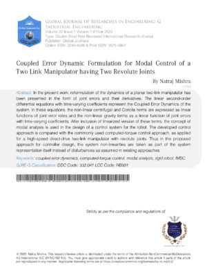MATHEMATICAL MODELLING The dynamics of a planar two-link rigid robot (Fig. 1) having two revolute joints is well explained in various text books on Robotics [1,2,42,43]. After considering the effects of payload and joint inertias, the matrix equation of motion of a two-link robot with revolute joints and a payload is given as follows. $$ \left\{ \begin{array}{l} \tau_ {1} \\\tau_ {2} \end{array} \right\} = \left[ \begin{array}{l l} M _ {1 1} & M _ {1 2} \\M _ {2 1} & M _ {2 2} \end{array} \right] \left\{ \begin{array}{l} \ddot {\theta} _ {1} \\\ddot {\theta} _ {2} \end{array} \right\} + \left[ \begin{array}{l} N _ {1} \\N _ {2} \end{array} \right] + \left[ \begin{array}{l} G _ {1} \\G _ {2} \end{array} \right] \quad (1) $$ where, $\tau_{1}$ and $\tau_{2}$ are joint torques, $\theta_{1}$ and $\theta_{2}$ are joint angles and $$ M _ {1 1} = (m _ {1} + m _ {2}) L _ {1} ^ {2} + m _ {2} L _ {2} ^ {2} + 2 m _ {2} L _ {1} L _ {2} \cos \theta_ {2} + I _ {h 1} + M _ {p} (L _ {1} ^ {2} + L _ {2} ^ {2} + 2 L _ {1} L _ {2} \cos \theta_ {2}) + m _ {h 2} L _ {1} ^ {2} $$ $$ M_{12} = M_{21} = m_{2} L_{2}^{2} + m_{2} L_{1} L_{2} \cos \theta_{2} + M_{p} (L_{1} L_{2} \cos \theta_{2} + L_{2}^{2}) $$ $$ M _ {2 2} = m _ {2} L _ {2} ^ {2} + I _ {h 2} + M _ {p} L _ {2} ^ {2} \tag {1a} $$ $$ N _ {1} = - m _ {2} L _ {1} L _ {2} \big (2 \dot {\theta} _ {1} \dot {\theta} _ {2} + \dot {\theta} _ {2} ^ {2} \big) \sin \theta_ {2} + M _ {p} L _ {1} L _ {2} \big (2 \dot {\theta} _ {1} \dot {\theta} _ {2} - \dot {\theta} _ {2} ^ {2} \big) \sin \theta_ {2} $$ $$ N _ {2} = m _ {2} L _ {1} L _ {2} \dot{\theta} _ {1} ^ {2} \sin \theta _ {2} - 2 M _ {p} L _ {1} L _ {2} \sin \theta _ {2} \cdot \dot{\theta} _ {1} \dot{\theta} _ {2} $$ $$ G _ {1} = \left(m _ {1} + m _ {h 2} + m _ {2} + M _ {p}\right) g L _ {1} \cos \theta_ {1} + \left(m _ {2} + M _ {p}\right) g L _ {2} \cos (\theta_ {1} + \theta_ {2}) $$ $$ G _ {2} = \left(m _ {2} + M _ {p}\right) g L _ {2} \cos \left(\theta _ {1} + \theta _ {2}\right) \tag{1c} $$ 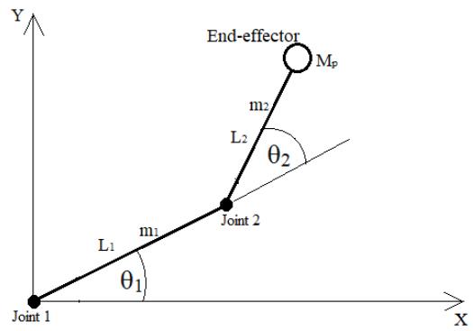 Fig. 1: A Two-Link Rigid serial robot having two Revolute Joints in X-Y plane In equation (1), $m_1$ and $m_2$ are masses of Link-1 and Link-2 respectively, $L_1$ and $L_2$ are lengths of Link-1 and Link-2 respectively, $l_{h1}$ and $l_{h2}$ are joint/hub mass moment of inertias at Joint-1 and Joint-2 respectively, $m_{h2}$ is the mass of hub of Joint-2 and $M_p$ is mass of payload attached at the end of Link 2, i.e., at the end-effector. $M_{11}, M_{12}, M_{21}$ and $M_{22}$ are the elements of inertia matrix, $N_1$ and $N_2$ are the elements of centrifugal/ Coriolis torque vector and $G_1$ and $G_2$ are the elements of the gravity torque vector. It can be seen from equation (1) that the mass matrix is coupled and depends upon the configuration of the manipulator. This makes the control problem difficult. To reduce this difficulty, Youcef and Harushiko [38] presented a design scheme that diagonalizes the mass matrix and also makes it configuration-invariant. In this work, a different approach is used which makes use of the original inertia of the robot. A robot is designed to move along the desired trajectory for performing an assigned task. Thus, the desired joint angles are $\theta_{1d}$ for Joint 1 and $\theta_{2d}$ for Joint 2. The joint errors will be as follows. $$ \theta_ {j e} = \theta_ {j d} - \theta_ {j} (2) $$ where, $j$ represents the joint number (=1, 2), subscript-'e' stands for 'error' and subscript-'d' stands for 'desired'. Next, we substitute for actual joint angles $\theta_{1}, \theta_{2}$ and their derivatives from equation (2) into equation (1). Firstly, we analyze the centrifugal/Coriolis' torque terms represented by $N_{1}$ and $N_{2}$. ### a) Analysis of Centrifugal/Coriolis Terms Equation (1b) can be re-written as: $$ N _ {1} = 2 L _ {1} L _ {2} \sin \theta _ {2} \left[ (M _ {p} - m _ {2}) \dot{\theta} _ {1} \dot{\theta} _ {2} - (m _ {2} + M _ {p}) \dot{\theta} _ {2} ^ {2} \right] $$ $$ N _ {2} = 2 L _ {1} L _ {2} \sin \theta_ {2} \left[ m _ {2} \dot {\theta} _ {1} ^ {2} - 2 M _ {p} \dot {\theta} _ {1} \dot {\theta} _ {2} \right] \tag {1b} $$ Using equation (2), we can write: $$ \dot{\theta}_1 \dot{\theta}_2 = (\dot{\theta}_{1d} - \dot{\theta}_{1e}) (\dot{\theta}_{2d} - \dot{\theta}_{2e}) = \dot{\theta}_{1d} \dot{\theta}_{2d} - \dot{\theta}_{1d} \dot{\theta}_{2e} - \dot{\theta}_{1e} \dot{\theta}_{2d} + \dot{\theta}_{1e} \dot{\theta}_{2e} $$ $$ \dot{\theta}_1^2 = (\dot{\theta}_{1d} - \dot{\theta}_{1e})^2 = \dot{\theta}_{1d}^2 + \dot{\theta}_{1e}^2 - 2 \dot{\theta}_{1d} \dot{\theta}_{1e} $$ $$ \dot {\theta} _ {2} ^ {2} = \left(\dot {\theta} _ {2 d} - \dot {\theta} _ {2 e}\right) ^ {2} = \dot {\theta} _ {2 d} ^ {2} + \dot {\theta} _ {2 e} ^ {2} - 2 \dot {\theta} _ {2 d} \dot {\theta} _ {2 e} $$ $$ \sin \theta_ {2} = \sin (\theta_ {2 d} - \theta_ {2 e}) = \sin \theta_ {2 d} \cos \theta_ {2 e} - \cos \theta_ {2 d} \sin \theta_ {2 e} $$ Substituting above expressions in equation (1b) we get $$ N_{1} = 2 L_{1} L_{2} (\sin \theta_{2d} \cos \theta_{2e} - \cos \theta_{2d} \sin \theta_{2e}) \big[\big( (M_{p} - m_{2}) \dot{\theta}_{1d} \dot{\theta}_{2d} - (m_{2} + M_{p}) \dot{\theta}_{2d}^{2} \big) \big] + \big\{ (m_{2} - m_{1}) \dot{\theta}_{1d} \dot{\theta}_{2d} - (m_{1} + M_{p}) \dot{\theta}_{2d}^{2} \big\} $$ $$ M _ {p}) \dot {\theta} _ {1 d} + 2 (m _ {2} + M _ {p}) \dot {\theta} _ {2 d} \} \dot {\theta} _ {2 e} - (M _ {p} - m _ {2}) \dot {\theta} _ {2 d} \dot {\theta} _ {1 e} + (M _ {p} - m _ {2}) \dot {\theta} _ {1 e} \dot {\theta} _ {2 e} - (m _ {2} + M _ {p}) \dot {\theta} _ {2 e} ^ {2} $$ $$ \begin{array}{l} N _ {2} = 2 L _ {1} L _ {2} (\sin \theta_ {2 d} \cos \theta_ {2 e} - \cos \theta_ {2 d} \sin \theta_ {2 e}) \big [ \big \{m _ {2} \dot {\theta} _ {1 d} ^ {2} - 2 M _ {p} \dot {\theta} _ {1 d} \dot {\theta} _ {2 d} \big \} + m _ {2} \dot {\theta} _ {1 e} ^ {2} - 2 M _ {p} \dot {\theta} _ {1 e} \dot {\theta} _ {2 e} \\+ \left(- 2 m _ {2} \dot {\theta} _ {1 d} + 2 M _ {p} \dot {\theta} _ {2 d}\right) \dot {\theta} _ {1 e} + 2 M _ {p} \dot {\theta} _ {1 d} \dot {\theta} _ {2 e} \biggr ] \\\end{array} $$ Assuming $\theta_{2e}$ to be very small, we can replace $\sin \theta_{2e}$ by $\theta_{2e}$ and $\cos \theta_{2e}$ by 1. Furthermore, for small joint errors and small joint error rates, we obtain $$ N _ {1} (t) = A (t) - \left(\frac {\partial A (t)}{\partial \theta_ {2 d} (t)}\right) \theta_ {2 e} (t); N _ {2} (t) = B (t) - \left(\frac {\partial B (t)}{\partial \theta_ {2 d} (t)}\right) \theta_ {2 e} (t) \qquad \qquad (3) $$ In above expressions, $$ A (t) = N _ {1 d} - 2 L _ {1} L _ {2} \sin \theta_ {2 d} \left[ \left(\frac {\partial \beta}{\partial \dot {\theta} _ {1 d}}\right) \dot {\theta} _ {1 e} + \left(\frac {\partial \beta}{\partial \dot {\theta} _ {2 d}}\right) \dot {\theta} _ {2 e} \right] \tag {3a} $$ $$ B(t) = N_{2d} - 2 L_1 L_2 \sin \theta_{2d} \left[ \left(\frac{\partial \gamma}{\partial \dot{\theta}_{1d}}\right) \dot{\theta}_{1e} + \left(\frac{\partial \gamma}{\partial \dot{\theta}_{2d}}\right) \dot{\theta}_{2e} \right] $$ $$ \beta (t) = \left(M _ {p} - m _ {2}\right) \dot {\theta} _ {1 d} \dot {\theta} _ {2 d} - \left(m _ {2} + M _ {p}\right) \dot {\theta} _ {2 d} ^ {2} \tag {3c} $$ $$ \gamma(t) = m_{2} \dot{\theta}_{1d}^{2} - 2 M_{p} \dot{\theta}_{1d} \dot{\theta}_{2d} $$ The terms, $\mathsf{N}_{1\mathrm{d}}$ and $\mathsf{N}_{2\mathrm{d}}$ can be obtained by replacing $\theta_{1}$ by $\theta_{1\mathrm{d}}$ and $\theta_{2}$ by $\theta_{2\mathrm{d}}$ in equation (1b). ### b) Analysis of Inertia Terms From equation (1), the inertia torques can be written as: $$ \left\{ \begin{array}{c} \text{if}_{1} \\ \text{if}_{2} \end{array} \right\} = \left[ \begin{array}{cc} M_{1 1} & M_{1 2} \\ M_{2 1} & M_{2 2} \end{array} \right] \left\{ \begin{array}{c} \ddot{\theta}_{1} \\ \ddot{\theta}_{2} \end{array} \right\} $$ Using equation (2), we can write: $$ \left\{ \begin{array}{l} if _ {1} \\ if _ {2} \end{array} \right\} = \left\{ \begin{array}{l} M _ {1 1} (\ddot{\theta} _ {1 d} - \ddot{\theta} _ {1 e}) + M _ {1 2} (\ddot{\theta} _ {2 d} - \ddot{\theta} _ {2 e}) \\ M _ {2 1} (\ddot{\theta} _ {1 d} - \ddot{\theta} _ {1 e}) + M _ {2 2} (\ddot{\theta} _ {2 d} - \ddot{\theta} _ {2 e}) \end{array} \right\} $$ In the above expression, the inertia terms: $\mathsf{M}_{11}$, $\mathsf{M}_{12}$, $\mathsf{M}_{21}$ and $\mathsf{M}_{22}$ can be obtained using equation (1a). These can be reformulated as follows. $$ M _ {1 1} = M _ {1 1 d} + \left[ a _ {1 1 d} \cos \theta_ {2 e} - \left(\frac {\partial a _ {1 1 d}}{\partial \theta_ {2 d}}\right) \sin \theta_ {2 e} \right]; $$ $$ M _ {1 2} = M _ {1 2 d} + \frac {1}{2} \Big [ a _ {1 1 d} \cos \theta_ {2 e} - \left(\frac {\partial a _ {1 1 d}}{\partial \theta_ {2 d}}\right) \sin \theta_ {2 e} \Big ] $$ $$ M _ {2 1} = M _ {2 1 d} + \frac{1}{2} \left[ a _ {1 1 d} \cos \theta_ {2 e} - \left(\frac{\partial a _ {1 1 d}}{\partial \theta_ {2 d}}\right) \sin \theta_ {2 e} \right] ; \, M _ {2 2} = M _ {2 2 d} \tag{4} $$ In above expressions, $$ M _ {1 1 d} = \left(m _ {1} + m _ {2} + m _ {h 2} + M _ {p}\right) L _ {1} ^ {2} + \left(m _ {2} + M _ {p}\right) L _ {2} ^ {2} + I _ {h 1}; $$ $$ M _ {1 2 d} = M _ {2 1 d} = \left(m _ {2} + M _ {p}\right) L _ {2} ^ {2}; $$ $$ M _ {2 2 d} = \left(m _ {2} + M _ {p}\right) L _ {2} ^ {2} + I _ {h 2}; a _ {1 1 d} = 2 L _ {1} L _ {2} \left(m _ {2} + M _ {p}\right) \cos \theta_ {2 d} \tag {4a} $$ Using equation (1) and equation (2), the inertia torques $(\mathrm{IF}_1$ and $\mathrm{IF}_2)$ acting at joints-1 and 2 can be written as: $$ \left\{ \begin{array}{l} \text{if}_{1} \\ \text{if}_{2} \end{array} \right\} = \left[ \begin{array}{ll} M_{1 1 d} & M_{1 2 d} \\ M_{2 1 d} & M_{2 2 d} \end{array} \right] \left\{ \begin{array}{l} \ddot{\theta}_{1 d} \\ \ddot{\theta}_{2 d} \end{array} \right\} + \left[ \begin{array}{ll} \phi & \frac{\phi}{2} \\ \frac{\phi}{2} & 0 \end{array} \right] \left\{ \begin{array}{l} \ddot{\theta}_{1 d} \\ \ddot{\theta}_{2 d} \end{array} \right\} - \left[ \begin{array}{ll} M_{1 1 d} + \phi & M_{1 2 d} + \frac{\phi}{2} \\ M_{2 1 d} + \frac{\phi}{2} & M_{2 2 d} \end{array} \right] \left\{ \begin{array}{l} \ddot{\theta}_{1 e} \\ \ddot{\theta}_{2 e} \end{array} \right\} $$ where $\phi = a_{11d}\cos \theta_{2e} - \left(\frac{\partial a_{11d}}{\partial\theta}\right)\sin \theta_{2e}$ ### c) Analysis of Gravity Terms The gravity terms are provided by equation (1c). Using equation (2), we can write: $$ \cos \theta_ {1} = \cos (\theta_ {1 d} - \theta_ {1 e}) = \cos \theta_ {1 d} \cos \theta_ {1 e} + \sin \theta_ {1 d} \sin \theta_ {1 e} $$ $$ \cos \theta_ {2} = \cos \left(\theta_ {2 d} - \theta_ {2 e}\right) = \cos \theta_ {2 d} \cos \theta_ {2 e} + \sin \theta_ {2 d} \sin \theta_ {2 e} $$ $$ \sin \theta_ {1} = \sin \left(\theta_ {1 d} - \theta_ {1 e}\right) = \sin \theta_ {1 d} \cos \theta_ {1 e} - \cos \theta_ {1 d} \sin \theta_ {1 e} $$ $$ \sin \theta_ {2} = \sin (\theta_ {2 d} - \theta_ {2 e}) = \sin \theta_ {2 d} \cos \theta_ {2 e} - \cos \theta_ {2 d} \sin \theta_ {2 e} $$ $$ \cos (\theta_ {1} + \theta_ {2}) = \cos \theta_ {1} \cos \theta_ {2} - \sin \theta_ {1} \sin \theta_ {2} $$ For very small values of $\theta_{1e}$ and $\theta_{2e}$, we can write $\cos \theta_{1e} \approx 1$; $\cos \theta_{2e} \approx 1$; $\sin \theta_{1e} \approx \theta_{1e}$, and $\sin \theta_{2e} \approx \theta_{2e}$. Thus, the gravity term can be rewritten as follows. $$ \left\{ \begin{array}{l} G _ {1} \\G _ {2} \end{array} \right\} = \left[ \begin{array}{l} G _ {1 d} \\G _ {2 d} \end{array} \right] + \left[ \begin{array}{l l} G _ {1 1 e} & G _ {1 2 e} \\G _ {2 1 e} & G _ {2 2 e} \end{array} \right] \left\{ \begin{array}{l} \theta_ {1 e} \\\theta_ {2 e} \end{array} \right\} \tag {5a} $$ In the above equation, $$ G _ {1 d} = \left(m _ {1} + m _ {h 2} + m _ {2} + M _ {p}\right) g L _ {1} \cos \theta_ {1 d} + \left(m _ {2} + M _ {p}\right) g L _ {2} \cos (\theta_ {1 d} + \theta_ {2 d}); $$ $$ G _ {2 d} = \left(m _ {2} + M _ {p}\right) g L _ {2} \cos (\theta_ {1 d} + \theta_ {2 d}) $$ $$ G _ {1 1 e} = \left(m _ {1} + m _ {h 2} + m _ {2} + M _ {p}\right) L _ {1} \sin \theta_ {1 d} + \left(m _ {2} + M _ {p}\right) L _ {2} \sin (\theta_ {1 d} + \theta_ {2 d}) $$ $$ G _ {1 2 e} = G _ {2 1 e} = G _ {2 2 e} = \left(m _ {2} + M _ {p}\right) L _ {2} \sin \left(\theta_ {1 d} + \theta_ {2 d}\right) \tag{5b} $$ ### d) Reformulated Dynamics Using equations- (1), (3), (4) and (5b) we can write, $$ \begin{array}{l} \left\{\tau_ {1 e} \atop \tau_ {2 e} \right\} = \left[ \begin{array}{c c} M _ {1 1 d} + \phi & M _ {1 2 d} + \frac {\phi}{2} \\M _ {2 1 d} + \frac {\phi}{2} & M _ {2 2 d} \end{array} \right] \left\{\ddot {\theta} _ {1 e} \atop \ddot {\theta} _ {2 e} \right\} - 2 L _ {1} L _ {2} (\theta_ {2 e}. \cos \theta_ {2 d} - \sin \theta_ {2 d}) \left[ \begin{array}{c c} \frac {\partial \beta}{\partial \dot {\theta} _ {1 d}} & \frac {\partial \beta}{\partial \dot {\theta} _ {2 d}} \\\frac {\partial \gamma}{\partial \dot {\theta}} & _ {2 d} \frac {\partial \gamma}{\partial \dot {\theta}} \end{array} \right] \left\{ \begin{array}{c} \dot {\theta} _ {1 e} \\\dot {\theta} _ {2 e} \end{array} \right\} - \\\left[ \begin{array}{l l} G _ {1 1 e} & G _ {1 2 e} \\G _ {2 1 e} & G _ {2 2 e} \end{array} \right] \left\{ \begin{array}{l} \theta_ {1 e} \\\theta_ {2 e} \end{array} \right\} \tag {6} \\\end{array} $$ In the above expression, $$ \tau_ {1 e} = \tau_ {1 d} - \tau_ {1} $$ $$ \tau_ {2 e} = \tau_ {2 d} - \tau_ {2} \tag {6a} $$ Since, equation (6) involves coupling between the joint errors, it is termed as 'Coupled-Error Dynamics'. In equation (6a), $$ \tau_ {1 d} = if _ {1 d} + N _ {1 d} + G _ {1 d}; \tau_ {2 d} = if _ {2 d} + N _ {2 d} + G _ {2 d} (6 b) $$ where, $IF_{1d} = M_{11d}\ddot{\theta}_{1d} + M_{12d}\ddot{\theta}_{2d}$; $IF_{2d} = M_{21d}\ddot{\theta}_{1d} + M_{22d}\ddot{\theta}_{2d}$; $N_{1d}$ and $N_{2d}$ are obtained by replacing variables- $\theta_{1}$ and $\theta_{2}$ in equation (1b) by $\theta_{1d}$ and $\theta_{2d}$; $G_{1d}$ and $G_{2d}$ are provided in equation (5b). ## III. CONTROL SYSTEM DESIGN Luh [39] proposed the design of a conventional controller for controlling each link or joint individually. In this paper, Modal Controller is used ([40], [41]) for the control function. In equation (6) the error dynamics of a two-link rigid robot is described. In general form, this equation can be written as $$ \left\{ \begin{array}{l} \tau_ {1 d} - \tau_ {1} \\\tau_ {2 d} - \tau_ {2} \end{array} \right\} = \left[ \begin{array}{l l} M _ {e 1 1} & M _ {e 1 2} \\M _ {e 2 1} & M _ {e 2 2} \end{array} \right] \left\{ \begin{array}{l} \ddot {\theta} _ {1 e} \\\ddot {\theta} _ {2 e} \end{array} \right\} - \left[ \begin{array}{l l} C _ {e 1 1} & C _ {e 1 2} \\C _ {e 2 1} & C _ {e 2 2} \end{array} \right] \left\{ \begin{array}{l} \dot {\theta} _ {1 e} \\\dot {\theta} _ {2 e} \end{array} \right\} - \left[ \begin{array}{l l} G _ {1 1 e} & G _ {1 2 e} \\G _ {2 1 e} & G _ {2 2 e} \end{array} \right] \left\{ \begin{array}{l} \theta_ {1 e} \\\theta_ {2 e} \end{array} \right\} $$ Defining the control torque as: $$ \{u \} = \{\tau \} = [ K _ {v} ] \left\{\dot {\theta} _ {e} \right\} + [ K _ {p} ] \left\{\theta_ {e} \right\} \tag {8} $$ and substituting in equation (7), we get $$ [M_{e}]{\dot{\theta}_{e}} + [K_{v}] - [C_{e}]{\dot{\theta}_{e}} + [K_{p}] - [G_{e}]{\theta_{e}} = {\tau_{d}} $$ In equation (9), the matrices- $\left[\mathbf{M}_{\mathrm{e}}\right]$, $\left[\mathbf{C}_{\mathrm{e}}\right]$ and $\left[\mathbf{G}_{\mathrm{e}}\right]$ are time-varying and also involve non-linear terms. It refers to the case of coupled control [41]. The values of gains- $\left[\mathbf{K}_{\mathrm{v}}\right]$ and $\left[\mathbf{K}_{\mathrm{p}}\right]$ must lie within a certain range so that the controller performance may not deteriorate even though the coefficients in equation (9) change with time. The ranges for $\left[\mathbf{K}_{\mathrm{v}}\right]$ and $\left[\mathbf{K}_{\mathrm{p}}\right]$ can be found out by designing the controller for minimum and maximum values of d and d as shown in the example below. Thereafter, the coefficients in equation (9) can be taken as constant. Now, the Eigenvalue problem for equation (9) can be written as: $$ \left[ M _ { e } \right] D ^ { 2 } \theta _ { e } + \left( \left[ K _ { p } \right] - \left[ G _ { e } \right] \right) \theta _ { e } = 0 \tag{ 1 0 } $$ Putting $D^2 = -\omega^2$ we get, $$ \left[ \left(K _ {p} - G _ {e}\right) - \omega^ {2} M _ {e} \right] \left\{\theta_ {e} \right\} = 0 \tag {11} $$ Let us assume, $\left[K_p\right] = \begin{bmatrix} K_{p11} & K_{p12}\\ K_{p21} & K_{p22} \end{bmatrix}$ (12) Now, we select $K_{p12} = G_{e12}$ and $K_{p21} = G_{e21}$. Thus we get, $$ \left(\left[ \begin{array}{c c} K _ {p 1 1} - G _ {1 1 e} & 0 \\0 & K _ {p 2 2} - G _ {2 2 e} \end{array} \right] - \omega^ {2} \left[ \begin{array}{c c} M _ {e 1 1} & M _ {e 1 2} \\M _ {e 2 1} & M _ {e 2 2} \end{array} \right]\right) \left\{\theta_ {1 e} \right\} = \left\{ \begin{array}{l} 0 \\0 \end{array} \right\} \tag {13} $$ Using equation (13), the frequency equation can be written as follows. $$ \left| \begin{array}{c c} K _ {p 1 1} - G _ {1 1 e} - \omega^ {2} M _ {e 1 1} & - \omega^ {2} M _ {e 1 2} \\- \omega^ {2} M _ {e 2 1} & K _ {p 2 2} - G _ {2 2 e} - \omega^ {2} M _ {e 2 2} \end{array} \right| = 0 ag {14} $$ From the frequency equation described by equation (14), two Eigenvalues $\omega_{1}^{2}$ and $\omega_{2}^{2}$ corresponding to 'mode I' and 'mode II' respectively, will be obtained. Using these eigenvalues, the eigenvectors can be found out. The eigenvectors for 'mode I' and 'mode II' can be expressed as follows. $$ \left(\frac{\theta_{2e}}{\theta_{1e}}\right)_{\mathrm{I}} = \sqrt{\frac{K_{p11} - G_{11e} - \omega_{1}^{2} M_{e11}}{K_{p22} - G_{22e} - \omega_{2}^{2} M_{e22}}} = r_{1}; \quad \left(\frac{\theta_{2e}}{\theta_{1e}}\right)_{\mathrm{II}} = \sqrt{\frac{K_{p11} - G_{11e} - \omega_{2}^{2} M_{e11}}{K_{p22} - G_{22e} - \omega_{2}^{2} M_{e22}}} = r_{2} \tag{15} $$ The modal matrix will now be given as: $$ [ W ] = \left[ \begin{array}{l l} 1 & 1 \\r _ {1} & r _ {2} \end{array} \right] = [ \begin{array}{l l} W _ {1} & W _ {2} \end{array} ] \tag {16} $$ This modal matrix is ortho-normalized using the relationship: WiTMeWi=1 where $i$ represents the modeumber and $\mathrm{Wi}^{\prime} = \mathrm{ciWi}$ $c_{j}$ being some constant. subscript 'T' means 'transpose'. The orthonormalized modal matrix is thus given as: $$ \begin{array}{l} [ W ^ {\prime} ] = [ c _ {1} \pmb {W _ {1}} c _ {2} \pmb {W _ {2}} ]; \mathrm {w h e r e ,} c _ {1} = [ M _ {e 1 1} + 2 r _ {1} M _ {e 1 2} + r _ {1} ^ {2} M _ {e 2 2} ] ^ {- 1}; \\c _ {2} = \left[ M _ {e 1 1} + 2 r _ {2} M _ {e 1 2} + r _ {2} ^ {2} M _ {e 2 2} \right] ^ {- 1} \tag {17} \\\end{array} $$ Now, let us take: $\{\theta_e\} = [W']\{\eta_e\}$ (18) where $\eta_{e}$ represents the modal coordinates. The variable $\theta_{e}$ represents the joint error and is in global coordinates. Substituting equation (18) into equation (9) and then multiplying throughout by $W^{T}$ we get: $$ [ W ^ {' T} M _ {e} W ^ {'} ] \{\ddot {\eta} _ {e} \} + [ W ^ {' T} (K _ {v} - C _ {e}) W ^ {'} ] \{\dot {\eta} _ {e} \} + \left[ W ^ {' T} \big (K _ {p} - G _ {e} \big) W ^ {'} \right] \{\eta_ {e} \} = [ W ^ {' T} ] \{\tau_ {d} \} $$ Now, $\left[W^{\prime T}M_{e}W^{\prime}\right] =$ identity matrix and $W^{\prime T}\big(K_p - G_e\big)W^{\prime} = \text{diagonal matrix containing Eigenvalues.}$ Thus, we get $$ \left[ \begin{array}{l l} 1 & 0 \\0 & 1 \end{array} \right] \left\{ \begin{array}{l} \ddot {\eta} _ {1 e} \\\ddot {\eta} _ {1 e} \end{array} \right\} + \left[ W ^ {\prime T} \left(K _ {v} - C _ {e}\right) W ^ {\prime} \right] \left\{ \begin{array}{l} \dot {\eta} _ {1 e} \\\dot {\eta} _ {2 e} \end{array} \right\} + \left[ \begin{array}{c c} \omega_ {1} ^ {2} & 0 \\0 & \omega_ {2} ^ {2} \end{array} \right] \left\{ \begin{array}{l} \eta_ {1 e} \\\eta_ {2 e} \end{array} \right\} = \left[ \begin{array}{c c} c _ {1} & c _ {1} r _ {1} \\c _ {2} & c _ {2} r _ {2} \end{array} \right] \left\{ \begin{array}{l} \tau_ {1 d} \\\tau_ {2 d} \end{array} \right\} \tag {19} $$ Now, let us assume that, $[K_v] = \begin{bmatrix} K_{v11} & K_{v12}\\ K_{v21} & K_{v22} \end{bmatrix}$ (20) Thus, $(K_{v} - C_{e}) = \begin{bmatrix} K_{v11} - C_{e11} & K_{v12} - C_{e12}\\ K_{v21} - C_{e21} & K_{v22} - C_{e22} \end{bmatrix}$ (21) Since $\left[\mathsf{C}_{\mathrm{e}}\right]$ is time-varying in nature, the matrix $(K_{\mathrm{v}} - C_{\mathrm{e}})$ will also be time-varying. It has been mentioned earlier that our task is to design a controller whose performance may not deteriorate due to a change in system parameters. For this, we design for either maximum or minimum values of $d$ and $d$. The joint error $\theta_{2\mathrm{e}}$ in equation (6) may be neglected if it is too small or otherwise its maximum allowable value may be used while designing the robotic system. In that case, the $C_{\mathrm{e}}$ matrix can be taken as constant and we shall obtain a range for gain $K_{\mathrm{v}}$. The off-diagonal terms in equation (21) can be chosen in the following two ways: 1. $\mathbf{K}_{\mathrm{v}12} = \mathbf{C}_{\mathrm{e}12}$ and $\mathbf{K}_{\mathrm{v}21} = \mathbf{C}_{\mathrm{e}21}$: In that case the off-diagonal terms will become zero. (22a) 2. $\mathbf{K}_{\mathrm{v12}} = -\mathbf{C}_{\mathrm{e21}}$ and $\mathbf{K}_{\mathrm{v21}} = -\mathbf{C}_{\mathrm{e12}}$: In that case both the off-diagonal terms will become equal and their values will be $-(C_{\mathrm{e12}} + C_{\mathrm{e21}})$. (22b) Using equation (22a), it will be possible to write: $$ \left([ K _ {v} ] - [ C _ {e} ]\right) = \alpha_ {1} \left[ M _ {e} \right] + \alpha_ {2} \left(\left[ K _ {p} \right] - \left[ G _ {e} \right]\right) \tag {23} $$ where $\alpha_{1}$ and $\alpha_{2}$ are some arbitrary constants. Thus, the second term in equation (19) will become $\left[ \begin{array}{cc}\alpha_{1} + \alpha_{2}\omega_{1}^{2} & 0\\ 0 & \alpha_{1} + \alpha_{2}\omega_{2}^{2} \end{array} \right].$ This may be written as: $\left[ \begin{array}{cc}2\xi_1\omega_1 & 0\\ 0 & 2\xi_2\omega_2 \end{array} \right]$ where $\xi_{1}$ and $\xi_{2}$ are modal damping ratios. The controller must exhibit non-oscillatory behavior to guarantee stability and for this, the minimum values of $\xi_{1}$ and $\xi_{2}$ should be 1 each. In that case, we obtain: $$ \alpha_ {1} = \frac{2 \omega_ {1} \omega_ {2}}{\omega_ {1} + \omega_ {2}} \text{and} \alpha_ {2} = \frac{2}{\omega_ {1} + \omega_ {2}} \tag{24} $$ Now, the relationship between gains- $K_{\mathrm{v}}$ and $K_{\mathrm{p}}$ can be obtained as follows. $$ \begin{array}{l} K _ {v 1 1} = \alpha_ {1} M _ {e 1 1} + \alpha_ {2} \big (K _ {p 1 1} - G _ {e 1 1} \big) + C _ {e 1 1} \\K _ {v 1 2} = \alpha_ {1} M _ {e 1 2} + C _ {e 1 2} \\K _ {v 2 1} = \alpha_ {1} M _ {e 2 1} + C _ {e 2 1} \\K _ {v 2 2} = \alpha_ {1} M _ {e 2 2} + \alpha_ {2} \left(K _ {p 2 2} - G _ {e 2 2}\right) + C _ {e 2 2} \tag {25} \\\end{array} $$ Similarly, equation (22b) can also be used to decouple the equation (9). This approach referred to as independent modal-space control (IMSC) [41] has been applied for a robotic system in the present work. ## IV. RESULTS AND DISCUSSIONS In this section, results based upon the control gains obtained using equations- (24) and (25) are presented. Based upon these results, a comparison of control effectiveness is done between Computed-Torque Control (CTC) ([1], [2], [42], [43], [44]) and Coupled-Error Dynamics (CED) approach. For this purpose, the serial robot (Fig. 1) is guided to follow a certain trajectory. The problem of formulation and optimization of trajectories is discussed by Lin et al. [45] while the control of manipulators using resolved-motion is discussed by Whitney [46] and Luh et al. [47]. The error equation for a 'computed-torque controller' is given as: $$ \left\{\ddot {\theta} _ {e} \right\} + \left[ K _ {v} \right] \left\{\dot {\theta} _ {e} \right\} + \left[ K _ {p} \right] \left\{\theta_ {e} \right\} = \left\{\tau_ {d} \right\} \tag {26} $$ Equation (26) is mostly used for 'independent joint control.' The gain matrices- $\left[\mathsf{K}_{\mathfrak{p}}\right]$ and $\left[\mathsf{K}_{\mathsf{v}}\right]$ are diagonal matrices and $\{d^{\prime}\}$ represents the vector of externally applied torque. A comparison of the equations (9) and (26) underlines the contribution of this work. The linearised versions of Coriolis, Gyroscopic and Gravity terms are now part of the control system matrices. Following relationship between $\mathsf{K}_{\mathsf{v}}$ and $\mathsf{K}_{\mathsf{p}}$ are used in CTC. $$ \operatorname {d i a g} \left[ K _ {v j} \right] = 2 \sqrt {\operatorname {d i a g} \left[ K _ {p j} \right]} \tag {27} $$ The method of finding the recommended control gain depends upon the natural frequency of the manipulator system [42]. The physical parameters used for the manipulator (Fig. 1) are provided in Table 1. Table 1: Physical parameters for Two-Link manipulator <table><tr><td>Symbol</td><td>Physical quantity</td><td>Value</td></tr><tr><td>L1</td><td>Length of link 1</td><td>0.5 m</td></tr><tr><td>L2</td><td>Length of link 2</td><td>0.5 m</td></tr><tr><td>m1</td><td>Mass of link 1</td><td>0.0312 kg</td></tr><tr><td>m2</td><td>Mass of link 2</td><td>0.0312 kg</td></tr><tr><td>Ih1</td><td>Hub inertia at joint 1</td><td>8 x 10-5kg·m2</td></tr><tr><td>Ih2</td><td>Hub inertia at joint 2</td><td>8 x 10-5kg·m2</td></tr><tr><td>Mp</td><td>Mass of payload</td><td>0.2 kg</td></tr></table> The error equation for 'coupled-error dynamics' is given by equation (9). The control problem requires that the end-effector of the robot must trace a straight line having equation: $y = 0.268x + 0.5$, in the X-Y plane (Fig. 2). For this, the joints of the robot must follow the desired Point-to-Point trajectories described by equation (28). Both the joints start from the initial orientation of $30^{\circ}$ at $t = 0$ second and reach the final orientations at $t = t_f = 20$ second. The joints start from rest at $t = 0$ second and come to rest at $t = t_f = 20$ second. $$ \theta_ {1 d} = 3 0 - \left(\frac {1 5 0}{t _ {f} ^ {3}}\right) t ^ {3} + \left(\frac {2 2 5}{t _ {f} ^ {4}}\right) t ^ {4} - \left(\frac {9 0}{t _ {f} ^ {5}}\right) t ^ {5}; $$ $$ \theta_ {2 d} = 3 0 + \left(\frac {7 5 0}{t _ {f} ^ {3}}\right) t ^ {3} - \left(\frac {1 1 2 5}{t _ {f} ^ {4}}\right) t ^ {4} + \left(\frac {4 5 0}{t _ {f} ^ {5}}\right) t ^ {5}; $$ $$ \dot {\theta} _ {1 d} = - \left(\frac {4 5 0}{t _ {f} ^ {3}}\right) t ^ {2} + \left(\frac {9 0 0}{t _ {f} ^ {4}}\right) t ^ {3} - \left(\frac {4 5 0}{t _ {f} ^ {5}}\right) t ^ {5}; $$ $$ \dot {\theta} _ {2 d} = \left(\frac {2 2 5 0}{t _ {f} ^ {3}}\right) t ^ {2} - \left(\frac {4 5 0 0}{t _ {f} ^ {4}}\right) t ^ {3} + \left(\frac {2 2 5 0}{t _ {f} ^ {5}}\right) t ^ {5} \tag {28} $$ In equation (28), $t_f$ represents the final value of time in which the joints reach their final orientations. The design conditions used for formulating these joint-space trajectories are provided in Table 2 below. Table 2: Design conditions for the formulation of joint-space trajectories <table><tr><td></td><td colspan="2">Joint 1</td><td colspan="2">Joint 2</td></tr><tr><td></td><td>t = 0 s</td><td>t = tf(20 s)</td><td>t = 0 s</td><td>t = tf(20 s)</td></tr><tr><td>Joint angular rotation</td><td>30°</td><td>15°</td><td>30°</td><td>105°</td></tr><tr><td>Joint angular speed</td><td>0°/s</td><td>0°/s</td><td>0°/s</td><td>0°/s</td></tr><tr><td>Joint angular acceleration</td><td>0°/s2</td><td>0°/s2</td><td>0°/s2</td><td>0°/s2</td></tr><tr><td>Maximum Joint speed</td><td colspan="2">-1.40625°/s (at t = 10 s)</td><td colspan="2">7.03125°/s (at t = 10 s)</td></tr><tr><td>Joint angle at maximum speed</td><td colspan="2">22.5°</td><td colspan="2">67.5°</td></tr></table> The angular rotations of the joints at $t = 0$ sec are found out using inverse kinematics at point P and point Q shown in Fig 2. The inverse kinematics relations for the planar Two-Link Rigid manipulator (Fig. 1) are given as follows: $$ \theta_ {2} = \cos^ {- 1} \left(\frac {\left(\sqrt {x ^ {2} + y ^ {2}}\right) ^ {2} - L _ {1} ^ {2} - L _ {2} ^ {2}}{2 L _ {1} L _ {2}}\right); \quad \theta_ {1} = \tan^ {- 1} \left(\frac {y}{x}\right) - \tan^ {- 1} \left(\frac {L _ {2} \sin \theta_ {2}}{L _ {1} + L _ {2} \cos \theta_ {2}}\right) \tag {29} $$ Fig. 2 shows the path traced by the end-effector of Two-Link Rigid manipulator in X-Y plane. 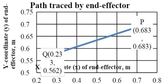 Fig. 2: Path traced by the end-effector of manipulator shown in Using Table 2, the design parameters for the CED-based controller involving the coefficients- $\left[\mathsf{M}_{\mathrm{e}}\right]$ $\left[\mathrm{C}_{\mathrm{e}}\right]$, and $\left[\mathrm{G}_{\mathrm{e}}\right]$ provided in equation (9) are found out to be as follows. $$ \begin{array}{l} M _ {e} = \left[ \begin{array}{c c} 0. 1 2 3 8 + 0. 0 4 4 2 \cos \theta_ {2 e} + 0. 1 0 6 8 \sin \theta_ {2 e} & 0. 0 5 7 8 + 0. 0 2 2 1 \cos \theta_ {2 e} + 0. 0 5 3 4 \sin \theta_ {2 e} \\0. 0 5 7 8 + 0. 0 2 2 1 \cos \theta_ {2 e} + 0. 0 5 3 4 \sin \theta_ {2 e} & 0. 0 5 7 9 \end{array} \right] \\C _ {e} = \left[ \begin{array}{l l} - 0. 0 0 5 2 \theta_ {2 e} + 0. 0 0 9 6 & 0. 0 1 1 6 \theta_ {2 e} - 0. 0 2 8 1 \\0. 0 1 0 7 \theta_ {2 e} - 0. 0 2 3 4 & - 0. 0 0 1 9 \theta_ {2 e} + 0. 0 0 4 5 \end{array} \right]; G _ {e} = \left[ \begin{array}{l l} 0. 1 6 5 8 & 0. 1 1 5 6 \\0. 1 1 5 6 & 0. 1 1 5 6 \end{array} \right] \tag {30} \\\end{array} $$ In equation (30), $\theta_{2\mathrm{e}}$ represents the joint error angle in Joint 2. The designer may check the accuracy required at the tip of the manipulator by selecting the value of $\theta_{2\mathrm{e}}$. Table 3 shows the control gains for the CED-based controller (based on equations- 24 and 25) and the CTC-based controller (based on equation (27)) for critically damped responses of the controllers. Table 3: Control gains for CED-based controller and CTC-based controller for critically damped response for the Two-Link Rigid manipulator <table><tr><td colspan="2">CED-based controller (equations- 24 and 25)</td><td>CTC-based controller (equation 27)</td></tr><tr><td>θ2e=0 radian</td><td>θ2e=0.1 radian</td><td></td></tr><tr><td>Kp=[289 0.1156 121]</td><td>Kp=[289 0.1156 121]</td><td rowspan="2">Kp=[289 0 121], Kv=[34 0 22]</td></tr><tr><td>Kv=[12.5539 3.8761 4.6529]</td><td>Kv=[12.8466 4.1178 4.5648]</td></tr></table> Table 3 provides the values of $K_{p}$ and $K_{v}$ matrices for CED-based and CTC-based controllers. The values in derivative gain matrix $K_{v}$ depend upon values in proportional gain matrix $K_{p}$ and also the level of accuracy required in case of CED-based controller. This level of accuracy is described by angle $\theta_{2e}$. On the other hand, in CTC-based controller, the values in $K_{v}$ matrix depend upon the values in $K_{p}$ matrix only. Once $K_{p}$ is fixed, $K_{v}$ also gets fixed. Thus, CED provides a facility to improve the transient response of the manipulator by changing the derivative gain $K_{v}$ based upon the uncertainty $\theta_{2e}$ present within the system. A comparison between the performances of CED-based controller and CTC-based controller is made below. Figure 3 is obtained by using the $K_{p}$ and $K_{v}$ matrices as provided in the first column of Table 3 for CED-based controller and third column for CTC-based controller. It can be seen that the positional accuracy of the end-effector obtained in case of CED-based controller lies very close to that of the CTC-based controller.  Fig. 3: Comparison of paths traced by end-effector of Two-Link Rigid robot in X-Y plane as obtained by CED and CTC (Table 3) Figures- 3a and 3b above, show the comparison between paths traced by the end-effector of Two-Link Rigid manipulator using both CED and CTC approaches. The desired path is shown by straight lines in the figures. From the figure, it can be seen that the positional accuracy of CED-based controller is very close to that of a CTC except that there are few fluctuations. A comparison between the control torques provided by CED and CTC is also done. Fig. 4(a) and Fig. 4(b) show the comparison between control torques provided by CED and CTC based controllers for the PD gains provided in Table 3 (column 1 and column 3). 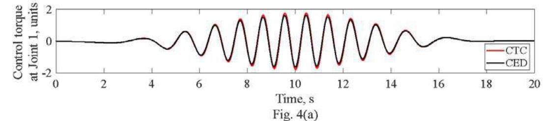 Fig. 1 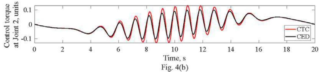 Fig. 4: Comparison between control torques provided by CED and CTC using control gains provided in columns 3 and 4 in Table 3 for the two-link rigid manipulator From Fig. 4(a) and Fig. 4(b), it can be observed that the control torque at Joint 1 is approximately same for the CED controller and CTC. For Joint 2, the control torque provided by CED controller is slightly lower than the CTC. The results show that the performance of CED-based controller is comparable to that of the CTC and hence it can be used for trajectory control of robotic manipulators with a great level of accuracy and precision. Now, effect of external disturbance on the performance of the proposed controller will be discussed. For this, a unit step load input is applied at both the joints and joint errors obtained using CED-based controller and CTC are compared with each other. It is found that when only PD gains are used, CTC has a better steady state response than the CED. In the presence of external disturbance, the joint errors in the CED-based controller are higher than that of CTC. It is due to the nature of dynamics. In CED, the joint error of one joint affects the accuracy of the other joint (equation 9) because in a serial robotic manipulator all the links are connected with each other and hence motion of each joint is affected by the motion of another joint. Since, this coupling effect is not there in the dynamics of CTC (equation 26), the joint errors are less. In order to reduce the joint errors in CED-based controller, integral gains are used. The method of calculating the integral gains are provided by equation (31) given below. $$ K _ {I i} = K _ {p i} \times K _ {v i} \tag {31} $$ In equation (31), $K_{Ii}$, $K_{pi}$ and $K_{vi}$ are the integral gain, proportional gain and derivative gain respectively for link $i$. Fig. 5 shows the joint errors under the influence of unit step load applied at both the joints obtained for CED-based controller and CTC when PID gains are used.   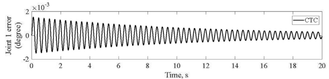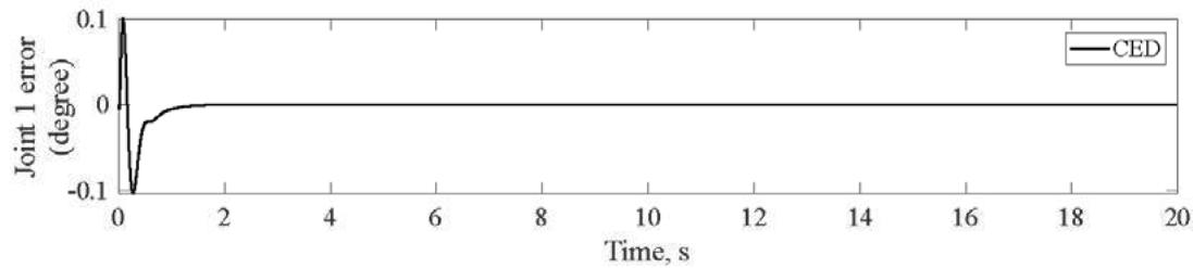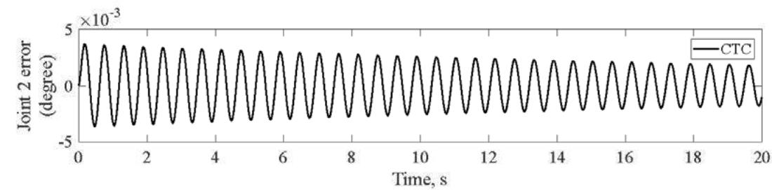 Fig. 5(a) 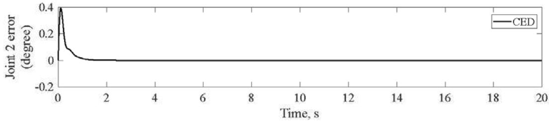 Fig. 5(b) From Fig. 5 it can be seen that due to introduction of integral gains, the joint errors are reduced to zero for the CED-based controller. For CTC also, the joint errors are significantly low but there are transients which decay with time. The only drawback with CED controller is that there is a high overshoot at the beginning. The control scheme based upon CED can be represented as shown below in Fig. 6. 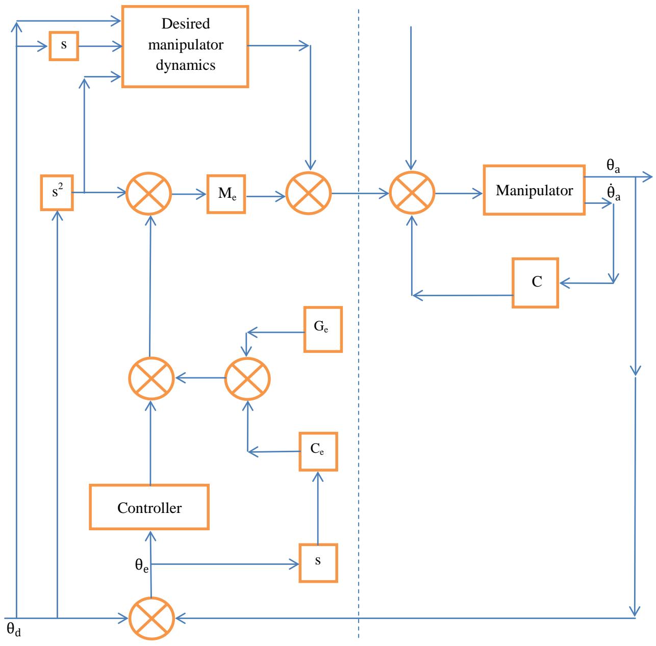 Fig. 6: Control scheme based upon Coupled-Error Dynamics (C = joint viscous damping) The control scheme shown in Fig. 6 has two portions: Servo-based portion and Model-based portion. The servo-based portion consists of the required controller that minimizes the joint errors for the manipulator. The manipulator forms the model-based portion. It is to be noted that the terms $C_e$ and $G_e$ used here correspond to a representative value of $\theta_d$ and are not actively changed. ## V. EFFECT OF LINK FLEXIBILITY ON CONTROLLER PERFORMANCE In this section, the effect of link flexibility on performance of the proposed controller is discussed. For this, the mathematical model of the two-link flexible manipulator [48] is developed. Fig. 7 shows a two-link flexible manipulator undergoing both rigid and flexible motions. 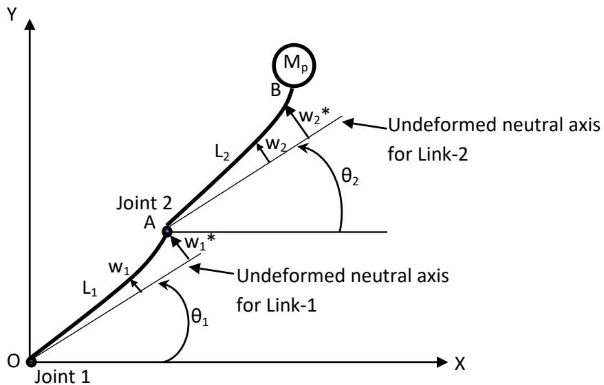 Fig. 7: Two Link Flexible manipulator Fig. 7 shows a two-link flexible manipulator undergoing small elastic deformations. The flexible links have lengths- $L_{1}$ and $L_{2}$. In the figure, $\theta_{1}$ and $\theta_{2}$ represent the rigid rotations, $w_{1}$ and $w_{2}$ represent the small flexural deformations of the flexible links and $w_{1}^{*}$ and $w_{2}^{*}$ represent the small flexural deformations at the end points of the links respectively. The governing equations of motion can be obtained by using Lagrangian dynamics. A detailed formulation is provided by Mishra et al. [50]. The expressions for joint torques can be represented as follows. $$ \tau_ {1} (t) = M _ {1 1} \ddot {\theta} _ {1} + M _ {1 2} \ddot {\theta} _ {2} + M _ {1 3} \ddot {w} _ {1} + M _ {1 4} \ddot {w} _ {2} + M _ {1 5} \ddot {w} _ {1} ^ {*} + M _ {1 6} \ddot {w} _ {2} ^ {*} + N _ {1} + G _ {1} + C _ {1 1} \dot {\theta} _ {1} + C _ {1 2} \dot {\theta} _ {2} + $$ $$ C _ {1 5} \dot {w} _ {1} ^ {*} + C _ {1 6} \dot {w} _ {2} ^ {*} + K _ {1 5} w _ {1} ^ {*} + K _ {1} ^ {\#} \tag {32a} $$ $$ \begin{array}{l} \tau_ {2} (t) = M _ {2 1} \ddot {\theta} _ {1} + M _ {2 2} \ddot {\theta} _ {2} + M _ {2 3} \ddot {w} _ {1} + M _ {2 4} \ddot {w} _ {2} + M _ {2 5} \ddot {w} _ {1} ^ {*} + M _ {2 6} \ddot {w} _ {2} ^ {*} + N _ {2} + G _ {2} + C _ {2 1} \dot {\theta} _ {1} + C _ {2 2} \dot {\theta} _ {2} + \\C _ {2 5} \dot {w} _ {1} ^ {*} + C _ {2 6} \dot {w} _ {2} ^ {*} + K _ {2 5} w _ {1} ^ {*} + K _ {2} ^ {\#} \tag {32b} \\\end{array} $$ In equation- (32), the terms M, N, G, C, K and $K^{\#}$ represent the inertia, centrifugal/Coriolis, gravity, gyroscopic/damping, stiffness and miscellaneous terms respectively. These expressions are derived after considering the bending angles at point A and point B (Fig. 7) as negligible. This is possible when the links have high flexural rigidity. The terms in equation (32) may be classified into rigid components and flexible components as follows. $$ \tau_ {1} (t) = \tau_ {1 _ {\text {r i g i d}}} + \tau_ {1 _ {\text {f l e x i b l e}}} \tag {33a} $$ $$ \tau_ {2} (t) = \tau_ {2 _ {\text {r i g i d}}} + \tau_ {2 _ {\text {f l e x i b l e}}} \tag {33b} $$ In equations- (32) and (33), the rigid components of joint torques (1_rigid and 2_rigid) are same as given in equation (1) provided the joint dampings $(C_{11}, C_{12}, C_{21}$ and $C_{22})$ are negligible. Rest other terms are considered under the category of flexible component of the joint torques (1Flexible and 2Flexible). In the proposed controller, the flexible components of joint torques act as the source of disturbance. The effect of link flexibility on the performances of the controllers in terms of end-effector position is shown in Fig. 8. The physical parameters of the flexible manipulator are same as for the rigid manipulator (Table 1) except the fact the values of flexural stiffness EI is taken as $1\mathrm{Nm}^2$ for both the links. 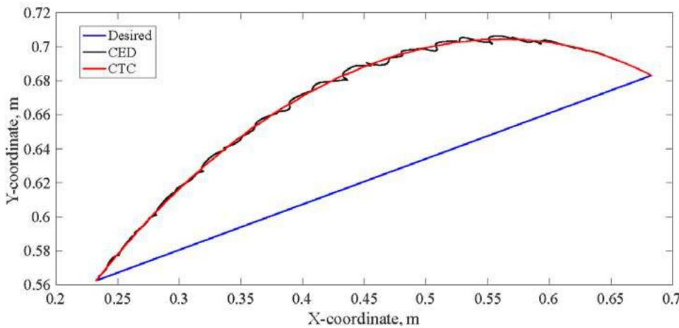 Fig. 8: Comparison of paths traced by end-effector of Two-Link Flexible robot in X-Y plane as obtained by CED and CTC From Fig. 8, it can be seen that due to the presence of flexibility in the links, the positional accuracy obtained by CED-based controller gets decreased than as shown in Fig. 3. There is only slight decrease in accuracy of the CTC-based controller when compared with Fig. 3. But, comparatively high values of control gains are used. The values of control gains used for the flexible manipulator are provided below in Table 4. Table 4: Control gains for CED-based controller and CTC-based controller for critically damped response for the Two-Link Flexible manipulator <table><tr><td>CED-based controller (equations- 24 and 25); (θ2e= 0 radian)</td><td>CTC-based controller (equation 27)</td></tr><tr><td>Kp = [324 0.1156 0.1156 144]</td><td>Kp = [324 0 0 144]</td></tr><tr><td>Kv = [13.3406 4.1638 4.1685 5.0547]</td><td>Kv = [36 0 0 24]</td></tr><tr><td>Ki = Kp × Kv</td><td>Ki = Kp × Kv</td></tr></table> The positional inaccuracy as observed in the response obtained by using CED-based controller is due to the effect of coupling between the joints of the flexible manipulator. The positional accuracy can be increased by increasing the values of control gains. Fig. 9 shows the comparison between the control torque requirements at the joints of the two-link flexible manipulator due to the CED and CTC-based controllers. It can be seen that the CED-based controller provides lesser control torques at the joints than the CTC-based controller. This is one reason why one obtains the good positional accuracy (Fig. 8) in case of CTC. But it is remarkable that the CED achieves the positional accuracy close to that of the CTC (Fig. 8) even at low values of control torques (Fig. 9). 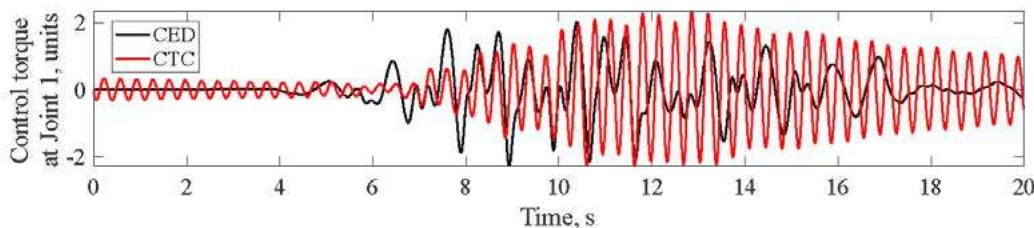 Fig. 5: Joint errors using PID gains under unit step disturbance for CED- based controller and CTC. (a) Joint 1 error, (b) Joint 2 error 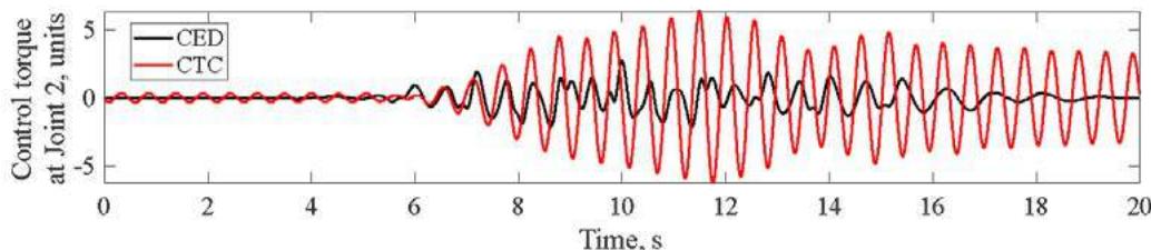 Fig. 9: Comparison between control torques provided by CED and CTC using control gains provided in Table 4 for the two-link flexible manipulator ## VI. CONCLUSIONS AND FUTURE DIRECTIONS In the present paper, the dynamics of a two-link rigid robot is reformulated as a coupled-error dynamics problem. This new equation retains the essence of original equation; it is non-linear and involves coupling between joint variables and also exhibits time and configuration dependent inertia. The centrifugal and Coriolis' torques vectors are expressed as linear function of joint error velocity $\{\dot{\theta}_e\}$. Similarly the gravity terms are expressed as linear functons of joint error in an approximate manner. An approach for deciding the control gains based upon modal parameters is presented. This helps in obtaining good performance from the controller even at low values of control gains. This results in low control torque requirement with improved positional accuracy of the robot simultaneously. On the other hand, it is advisable to use CTC when joint inertias are negligible [48] and when all the dynamic parameters of the given system are known with certainty [49]. The results presented in this paper are based upon simulation and include the effects of both the link and joint inertias and external disturbance. It is shown that the proposed controller based upon coupled-error dynamics scheme yields promising results in the presence of both internal disturbance in the form of link flexibility and external disturbance. In future, it is required to perform experiments and validate the results. Furthermore, the performance of the controller is shown by using polynomial trajectories. It is required to check the effect of various other types of trajectories on the performance of CED-based controller.

Generating HTML Viewer...

References

50 Cites in Article
Frank Lewis,Darren Dawson,Chaouki Abdallah (2004). Robot Manipulator Control.
M Spong,S Hutchinson,M Vidyasagar Robot Modelling and Control.
M Spong,M Vidyasagar (1987). Robust linear compensator design for nonlinear robotic control.
Romeo Ortega,Mark Spong (1989). Adaptive motion control of rigid robots: A tutorial.
N Mcclamroch,W Danwei (1988). Feedback stabilization and tracking of constrained robots.
Jacques Jean-,Hyun Slotine,Yang (1989). Improving the efficiency of time-optimal path-following algorithms.
K Youcef-Toumi,A Kuo (1993). High-speed trajectory control of a direct-drive manipulator.
Ou Ma,Jorge Angeles (1993). Optimum design of manipulators under dynamic isotropy conditions.
Aurelio Antonio,V (2000). Global minimum-jerk trajectory planning of robot manipulators.
D Constantinescu,E Croft (2000). Smooth and timeoptimal trajectory planning for industrial manipulators along specified paths.
A Gasparetto,V Zanotto (2007). A new method for smooth trajectory planning of robot manipulators.
P Marcello,B Giovanni,B Federico (2015). On designing optimal trajectories for servo-actuated mechanisms: detailed virtual prototyping and experimental evaluation.
B Xavier,S Daniel,N Khoi (2010). From motion planning to trajectory control with bounded jerk for service manipulator robots.
J Machado,J De Carvalho,A Galhano (1993). Analysis of robot dynamics and compensation using classical and computed torque techniques.
Zvi Shiller,Hai Chang (1995). Trajectory Preshaping for High-Speed Articulated Systems.
C Muller-Karger,A Leonell Granados Mirena,J Scarpati Lopez (2000). Hyperbolic trajectories for pick-and-place operations to elude obstacles.
P Ouyang,Q Li,W Zhang (2003). Integrated design of robotic mechanisms for force balancing and trajectory tracking.
Behrouz Afzali-Far,Per Lidstrom,Anders Robertsson (2016). Dynamic isotropy in 3-DOF Gantry Tau robots - an analytical study.
V Arakelian,Y Aoustin,C Chevallereau (2016). On the Design of the Exoskeleton Arm with Decoupled Dynamics.
Vigen Arakelian,Jiali Xu,Jean-Paul Le Baron (2016). Mechatronic design of adjustable serial manipulators with decoupled dynamics taking into account the changing payload.
A Al-Gburi,C Freeman,M French (2017). Gap-metric-based robustness analysis of nonlinear systems with full and partial feedback linearisation.
Haleema Asif,Ali Nasir,Umar Shami,Syed Rizvi,Muhammad Gulzar (2017). Design and comparison of linear feedback control laws for inverse Kinematics based robotic arm.
Soonwoong Hwang,Hyeonguk Kim,Younsung Choi,Kyoosik Shin,Changsoo Han (2017). Design optimization method for 7 DOF robot manipulator using performance indices.
V Arakelian,J Xu,J Le Baron (2018). Dynamic Decoupling of Robot Manipulators: A Review with New Examples.
Zhifeng Liu,Jingjing Xu,Qiang Cheng,Yongsheng Zhao,Yanhu Pei,Congbin Yang (2018). Trajectory Planning with Minimum Synthesis Error for Industrial Robots Using Screw Theory.
Amruta Rout,M Dileep,Golak Mohanta,Bbvl Deepak,B Biswal (2018). Optimal time-jerk trajectory planning of 6 axis welding robot using TLBO method.
Y Hou,M Mason (2019). Criteria for Maintaining Desired Contacts for Quasi-static Systems.
Stefan Friedrich,Martin Buss (2019). Parameterizing robust manipulator controllers under approximate inverse dynamics: A double‐Youla approach.
Lei Lu,Jiong Zhang,Jerry Fuh,Jiang Han,Hao Wang (2020). Time-optimal tool motion planning with tool-tip kinematic constraints for robotic machining of sculptured surfaces.
Marin Kobilarov (2014). Nonlinear Trajectory Control of Multi-body Aerial Manipulators.
F Wu,W Zhang,Q Li,P Ouyang (2002). Integrated Design and PD Control of High-Speed Closed-loop Mechanisms.
Juan Cambera,Vicente Feliu-Batlle (2017). Input-state feedback linearization control of a single-link flexible robot arm moving under gravity and joint friction.
Bao Rong,Xiaoting Rui,Kun Lu,Ling Tao,Guoping Wang,Xiaojun Ni (2018). Transfer matrix method for dynamics modeling and independent modal space vibration control design of linear hybrid multibody system.
Gang Shen,Ge Li,Wanshun Zang,Xiang Li,Yu Tang (2019). Modal Space Feedforward Control for Electro-Hydraulic Parallel Mechanism.
Jing-Zhou Zhao,Guo-Feng Yao,Rui-Yao Liu,Yuan-Cheng Zhu,Kui-Yang Gao,Min Wang (2020). Interval Analysis of the Eigenvalues of Closed-Loop Control Systems with Uncertain Parameters.
K Toumi,H Asada (1987). The design of open-loop manipulator arms with decoupled and configurationinvariant inertia tensors.
J Luh (1983). Conventional controller design for industrial robots — A tutorial.
S Rao Mechanical Vibrations.
Meirovitch Leonard Dynamics and Control of Structures.
Srishti Rawal,Aswini Madhubalan,Puviyarasu Manikandan,Jagadeesh Kanna (2003). Study on the Design of Space Gloves and EVA Suits with Future Challenges.
Gauri Agarwal,Alpana Razdan,Rakesh Samal,Vandana Sharma,Shikha Koul,Vandana Mishra (2014). Genetic Signatures of Chromosome 20 Mosaicism in Recurrent Pregnancy Loss.
S Rattan,B Nakra,J Shah (2015). Dynamic analysis of two link robot manipulator for control design using computed torque control.
C Lin,P Chang,J Luh (1983). Formulation and optimization of cubic polynomial joint trajectories for industrial robots.
Daniel Whitney (1969). Resolved Motion Rate Control of Manipulators and Human Prostheses.
J Luh,M Walker,R Paul (1980). Resolved-acceleration control of mechanical manipulators.
Mohamed Mehrez,Ayman El-Badawy (2010). Effect of the joint inertia on selection of under-actuated control algorithm for flexible-link manipulators.
Eshita Rastogi,Lal Prasad (2015). Comparative performance analysis of PD/PID computed torque control, filtered error approximation based control and NN control for a robot manipulator.
S Natraj Mishra,B Singh,Nakra (2015). Dynamic modelling of two link flexible manipulator using Lagrangian assumed modes method.
No ethics committee approval was required for this article type.
Data Availability
Not applicable for this article.
How to Cite This Article
Natraj Mishra. 2026. \u201cCoupled Error Dynamic Formulation for Modal Control of a Two Link Manipulator Having Two Revolute Joints\u201d. Global Journal of Research in Engineering - G: Industrial Engineering GJRE-G Volume 22 (GJRE Volume 22 Issue G1).
Explore published articles in an immersive Augmented Reality environment. Our platform converts research papers into interactive 3D books, allowing readers to view and interact with content using AR and VR compatible devices.
Your published article is automatically converted into a realistic 3D book. Flip through pages and read research papers in a more engaging and interactive format.
Our website is actively being updated, and changes may occur frequently. Please clear your browser cache if needed. For feedback or error reporting, please email [email protected]
Thank you for connecting with us. We will respond to you shortly.