## I. RESEARCH BACKGROUND a) The blackbody radiation issue in the history: Rayleigh-Jeans formula and oscillator model In the classic statistical theory, the thermal radiation is thought to be the electromagnetic wave. Accordingly, the thermal radiation energy in different frequency in the blackbody cavity is given. The Maxwell equations in the vacuum is written as follows, $$ \nabla \cdot \vec {E} = 0, \nabla \times \vec {H} - \frac {1}{c} \frac {\partial \vec {E}}{\partial t} = 0, \tag {1} $$ $$ \nabla \cdot \vec{H} = 0,\nabla \times \vec{E} + \frac{1}{c} \frac{\partial \vec{H}}{\partial t} = 0.\tag{2} $$ Here, $\vec{E},\vec{H}$ are the electric and magnetic fields, respectively, and c is the velocity of light in vacuum. Utilizing the curl of electromagnetic fields, the above four electromagnetic field equations are combined into the following two vector-type wave equations. $$ \nabla^ {2} \vec {E} - \frac {1}{c ^ {2}} \frac {\partial^ {2} \vec {E}}{\partial t ^ {2}} = 0, \tag {3} $$ $$ \nabla^ {2} \vec {H} - \frac {1}{c ^ {2}} \frac {\partial^ {2} \vec {H}}{\partial t ^ {2}} = 0. \tag {4} $$ In total, six scalar equations are included in the above two vector wave equations, representing the six components of electromagnetic fields, i.e., $E_x, E_y, E_z$, $H_x, H_y, H_z$, re spectively. Correspondingly, each scalar equation can be written into one standard equation that is used to solve a representative variable, $\varphi$. $$ \nabla^ {2} \varphi - \frac {1}{c ^ {2}} \frac {\partial^ {2} \varphi}{\partial t ^ {2}} = 0. (5) $$ Assume the boundaries of the cavity that surrounds the thermal radiation fields consist of three pairs of planar surfaces, i.e., $$ \mathrm {x} = 0, \alpha ; \mathrm {y} = 0, \beta ; \mathrm {z} = 0, \gamma . \tag {6} $$ Then, the volume of blackbody cavity is given as $$ V = \alpha \beta \gamma . \tag {7} $$ For a simple computation, the vector potential, $\vec{A}$, is introduced based on the Coulomb gauge. Then, the following formulae are obtained. $$ \vec {H} = \nabla \times \vec {A}, \vec {E} = - \frac {1}{c} \frac {\partial \vec {A}}{\partial t}. \tag {8} $$ It is noted that the vector potential satisfies the wave equation as well. $$ \nabla^ {2} \vec {A} - \frac {1}{c ^ {2}} \frac {\partial^ {2} \vec {A}}{\partial t ^ {2}} = 0. \tag {9} $$ Next, the electromagnetic wave is decomposed into the superposition of vibrations of different frequencies. Concretely, the wave equation of one component of vector potential, e.g., $A_{x}$, is solved by means of the method of variable separation. The vector potential $A_{x}$ is written into the formula below based on the principle of separation. $$ A _ {x} = f (t) X (x) Y (y) Z (z). \tag {10} $$ At the separation, the following four sub- equations of $A_{x}$ are obtained. $$ \frac{1}{X} \frac{d^{2} X}{d x^{2}} = - p^{2}, \frac{1}{Y} \frac{d^{2} Y}{d y^{2}} = - q^{2}, \frac{1}{Z} \frac{d^{2} Z}{d z^{ 2}} = - r^{2}, \frac{1}{f} \frac{d^{2} f}{d t^{2}} = - \omega^{2}. (11) $$ And, the four separating constants satisfy the relation below. $$ p ^ {2} + q ^ {2} + r ^ {2} = \frac {\omega^ {2}}{c ^ {2}}. \tag {12} $$ The detail is omitted here (see Ref. [1]). Through the similar procedure, the three components of vector potential deduced are achieved as below. $$ A _ {x} = \sum_ {l, m, n} f (t) A \cos \frac {l \pi x}{\alpha} \sin \frac {m \pi y}{\beta} \sin \frac {n \pi z}{\gamma}, \tag {13} $$ $$ A _ {y} = \sum_ {l, m, n} f (t) B \sin \frac {l \pi x}{\alpha} \cos \frac {m \pi y}{\beta} \sin \frac {n \pi z}{\gamma}, \tag {14} $$ $$ A _ {z} = \sum_ {l, m, n} f (t) C \sin \frac {l \pi x}{\alpha} \sin \frac {m \pi y}{\beta} \cos \frac {n \pi z}{\gamma}. \tag {15} $$ Here, A, B, C are undetermined coefficients. The values of parameters, l, m, n, can only be positive integer or zero. Besides, the two set of parameters, p, q, r and l, m, n satisfy the following relation. $$ p = \frac {l \pi}{\alpha}, q = \frac {m \pi}{\beta}, r = \frac {n \pi}{\gamma}. \tag {16} $$ Inserting Eq. (16) into Eq. (12), the below equality is obtained. $$ \frac {l ^ {2}}{\alpha^ {2}} + \frac {m ^ {2}}{\beta^ {2}} + \frac {n ^ {2}}{\gamma^ {2}} = \frac {\omega^ {2}}{\pi^ {2} c ^ {2}} = \frac {4 v ^ {2}}{c ^ {2}}. \tag {17} $$ The above identity is related to the ellipsoidal function. Then, according to the volume of ellipsoid, the freedom number of vibrations between $\nu$ and $\nu +\mathrm{d}\nu$, i.e., $g(\nu)\mathrm{d}\nu$, is given. $$ \mathrm {g} (\mathrm {v}) \mathrm {d v} = \frac {8 \pi V}{c ^ {3}} v ^ {2} d v. \tag {18} $$ According to the classic electrodynamics, the energy of radiation field, i.e., electromagnetic wave, which is defined as EN, is $$ \mathrm{EN} = \frac{1}{8\pi} \int (\overrightarrow{E}^{2} + \overrightarrow{H}^{2}) \, d\tau . \tag{19} $$ Here, $\mathrm{d}\tau = \mathrm{d}x\cdot \mathrm{d}y\cdot \mathrm{d}z$, is the volume element. According to Eq. (8), the electromagnetic fields can be calculated through the vector potential that is expressed in Eqs. (13-15). Inserting the electromagnetic fields into the above integral, and after integration, the energy EN, is written as $$ \mathrm{EN} = \frac{V}{64\pi c^{2}} \sum_{l,m,n} \left\{\left(\frac{df}{dt}\right)^{2} + \omega^{2} f^{2}\right\} \left(A^{2} + B^{2} + C^{ 2}\right). $$ It is seen from the above formula that the energy of radiation can be expressed as the sum of each vibration freedom. Assume the energy of one vibration freedom is $\varepsilon$, and it equals to $$ \varepsilon = \frac {V}{6 4 \pi c ^ {2}} (A ^ {2} + B ^ {2} + C ^ {2}) \left\{\left(\frac {d f}{d t}\right) ^ {2} + \omega^ {2} f ^ {2} \right\}. \tag {21} $$ Then, we define one new parameter, $Q$, and express it as follow. $$ Q ^ {2} = \frac {V}{3 2 \pi c ^ {2}} \left(A ^ {2} + B ^ {2} + C ^ {2}\right) f ^ {2}, \tag {22} $$ The following relation can be achieved. $$ \varepsilon = \frac{1}{2} \dot{Q}^{2} + \frac{1}{2} \omega^{2} Q^{2}. $$ This is the same with the energy expression of linear oscillator model (with the mass of oscillator set as $m = 1$ ). Here, $Q$ represents the displacement of oscillator and is one equivalent generalized coordinate. Correspondingly, the generalized momentum is $P = \dot{Q}$. As seen, the radiation field can be treated as the mechanic system that consists of many harmonic oscillators. So, the radiation energy in the interval between $\nu$ and $\nu + \mathrm{dv}$ can be expressed as below. $$ E_{\nu}d\nu = \bar{\varepsilon}g(\nu)d\nu = \frac{8\pi V}{c^{3}}kT\nu^{2}d\nu. $$ This is the famous Rayleigh-Jeans radiation formula. Here, $\bar{\varepsilon} = kT$, which represents the mean energy of oscillator and is given through the law of energy equipartition in the classic statistical mechanics. b) Linear fluid wave theory of plasma: continuum and "small" disturbance[2] In plasma physics, the ionic fluid momentum equation when excluding the effects of magnetic field and collision can be expressed as $$ M n \left[ \frac {\partial \vec {v _ {l}}}{\partial t} + (\vec {v _ {l}} \cdot \nabla) \vec {v _ {l}} \right] = e n \vec {E} - \nabla p = - e n \nabla \phi - \gamma_ {i} K T _ {i} \nabla n. \tag {25} $$ Utilizing the linear approximation, i.e., ignoring the quadratic (nonlinear) disturbance of convection which is the second term of Eq. (23) left, and the planar wave of small disturbance, we have $$ - i \omega M n _ {0} v _ {i 1} = - e n _ {0} i k \phi_ {1} - \gamma_ {i} K T _ {i} i k n _ {1}. \tag {26} $$ At the assumption of electric neutrality and the Boltzmann equilibrium of electron with electric potential, the relation between the disturbed density and potential is obtained. $$ n _ {1} = n _ {0} \frac {e \phi_ {1}}{K T _ {e}}. (2 7) $$ Here, $n_0$ is the undisturbed background ion density. Furthermore, the continuity equation of ion fluid is expressed below. $$ \frac {\partial n}{\partial t} + \nabla \cdot n \vec {v _ {l}} = 0. \tag {28} $$ Similarly, at the linear approximation and planar wave of small disturbance, we have $$ \mathrm {i} \omega n _ {1} = n _ {0} i k v _ {i 1}. \tag {29} $$ Last, the ionic acoustic speed is achieved based on the above three disturbance formulae, Eqs. (24, 25, 27). $$ \frac {\omega}{k} = \left(\frac {K T _ {e} + \gamma_ {i} K T _ {i}}{M}\right) ^ {1 / 2} \equiv v _ {s}. \tag {30} $$ ### c) The dispersion relation of ionic acoustic wave[2] The electric neutrality assumption is discarded, and the Poisson's equation at the linear and small wave approximations is considered as below. $$ \varepsilon_ {0} \nabla \cdot \overrightarrow {E _ {1}} = \varepsilon_ {0} k ^ {2} \phi_ {1} = e \left(n _ {i 1} - n _ {e 1}\right). \tag {31} $$ Here, the disturbed electron density is still given by the Boltzmann relation, i.e., $$ n _ {e 1} = \frac {e \phi_ {1}}{K T _ {e}} n _ {0}. \tag {32} $$ The disturbed ion density is still given by its continuity equation, which couples the disturbed ion velocity. $$ \mathrm {i} \omega n _ {i 1} = n _ {0} i k v _ {i 1}. \tag {33} $$ And, the disturbance relation given by the momentum equation is still existed, i.e., $$ -i\omega M n_{0} v_{i1} = -e n_{0} i k \phi_{1} - \gamma_{i} K T_{i} i k n_{i1}. $$ Accordingly, the above four disturbance relations at the more exact condition, i.e., the quasi-neutrality of plasma is not applied, cooperatively give rise to the dispersion of ionic wave. $$ \frac {\omega}{k} = \left(\frac {K T _ {e}}{M} \frac {1}{1 + k ^ {2} \lambda_ {D} ^ {2}} + \frac {\gamma_ {i} K T _ {i}}{M}\right) ^ {1 / 2}. \tag {35} $$ Here, $\lambda_{D} = \left(\frac{\varepsilon_{0}KT_{e}}{n_{0}e^{2}}\right)^{1 / 2}$ and is the famous Debye constant of plasma that shields the non-neutral region in plasma. ### d) Planar wave and oscillator at small disturbance $$ \overrightarrow {v _ {i 1}} = v _ {i 1} \exp (i k x - i \omega t) \hat {\vec {x}}, \tag {36} $$ $$ n _ {1} = n _ {1} \exp (i k x - i \omega t), \tag {37} $$ $$ \overrightarrow {E _ {1}} = E _ {1} \exp (i k x - i \omega t) \hat {\vec {x}}. \tag {38} $$ As seen, the planar wave of small disturbance can be treated as oscillator. All the above contents summarize the wave characteristic of mass. Namely, it fluctuates at small disturbance. This is caused by the oscillator model at the continuum, or more precisely when the interaction of mass is continuative. ## II. INNOVATION AND BREAKTHROUGH # a) The It is well-known that the prediction of Rayleigh-Jeans formula for the blackbody radiation is in good agreement with experimental measurement at low frequency terminal but fails at the high frequency terminal, even diverging. To solve this so-called ultraviolet disaster, Planck put forward to the idea that the energy of oscillator in the blackbody cavity is quantized, i.e., the energy of each oscillator can only be the integer times of one minimum, which is expressed as $$ \varepsilon = h v. \tag {39} $$ Here, the parameter $h$ is thereby called the Planck's constant. Then, at certain temperature $T$ and the Boltzmann distribution, the appearing probability of modulus with the energy, $\varepsilon_{n} = nh\nu$, is expressed as $$ p _ {n} = \frac {\exp (- \beta \varepsilon_ {n})}{\sum_ {n = 0} ^ {\infty} \exp (- \beta \varepsilon_ {n})}, \beta = \frac {1}{k T}. \tag {40} $$ At the proposal of energy quantization, the mean energy of oscillators now becomes $$ \bar {\varepsilon} = \sum_ {n = 0} ^ {\infty} p _ {n} \varepsilon_ {n} = \frac {\varepsilon}{\exp (\beta \varepsilon) - 1} = \frac {h \nu}{\exp \left(\frac {h \nu}{k T}\right) - 1}. \tag {41} $$ Replacing the old mean energy formula of oscillator in the Rayleigh-Jeans formula with the above new one, we get the Planck's formula below, which is in accord to the experiments at both the low- and high- frequency terminals. $$ E _ {\nu} = \frac {8 \pi V \nu^ {2}}{c ^ {3}} \frac {h \nu}{\exp \left(\frac {h \nu}{k T}\right) - 1}. \tag {42} $$ It is noted that the Planck's formula can return to the Rayleigh-Jeans formula at the limit of high temperature or equivalently at the limit of low frequency, i.e., when KT $\gg$ hv, the quantized mean energy of oscillator approximates to the continuum one, as illustrated below. $$ \bar {\varepsilon} = \frac {h \nu}{e x p \left(\frac {h \nu}{K T}\right) - 1} \approx \frac {h \nu}{0 + \frac {h \nu}{K T} + \frac {1}{2 !} \left(\frac {h \nu}{K T}\right) ^ {2} + \cdots} \approx K T \left(\frac {1}{1 + \frac {1 h \nu}{2 ! K T}}\right) \approx K T \left[ 1 - \frac {1}{2 !} \left(\frac {h \nu}{K T}\right) + \dots \right] \approx K T. (4 3) $$ According to Eq. (43), it can be concluded that the blackbody radiation at the low frequency limit that is presented by the Rayleigh-Jeans formula exhibits the wave characteristic while at high frequency limit, it behaves more like particles. b) Nonlinear solitary wave theory of plasma, i.e., KdV equation[3] Considering the continuity and momentum equations of ion fluid that couple the nonlinear terms, the Poisson's equation and the Boltzmann distribution of electron fluid, we have the following partial differential equation set. $$ \frac {\partial n}{\partial t} + \frac {\partial}{\partial x} (n u) = 0, \tag {44} $$ $$ \frac {\partial u}{\partial t} + u \frac {\partial u}{\partial x} = - \frac {e}{M} \frac {\partial \phi}{\partial x}, \tag {45} $$ $$ \mathrm {k} T _ {e} \frac {\partial n _ {e}}{\partial x} = e n _ {e} \frac {\partial \phi}{\partial x}, \tag {46} $$ $$ \varepsilon_ {0} \frac{\partial^ {2} \phi}{\partial x ^ {2}} = e \left(n _ {e} - n\right). $$ For the convenience of derivation of the formula, the non-dimensional process toward the above equation set is needed, by means of the below characteristic quantities, i.e., the normalized undisturbed density $n_0$, normalized ionic acoustic speed, $(kT_e / M)^{1/2}$, normalized plasma Debye length, $\lambda_D = \sqrt{\frac{\varepsilon_0 kT_e}{e^2 n_0}}$, normalized electric potential, $\frac{kT_e}{e}$, and the normalized plasma collective vibration time scale, $\omega_{p,i}^{-1} = \sqrt{\frac{\varepsilon_0 M}{e^2 n_0}}$. After this process, we obtain the normalized fluid model below. $$ \frac {\partial n ^ {\prime}}{\partial t ^ {\prime}} + \frac {\partial}{\partial x ^ {\prime}} \left(n ^ {\prime} u ^ {\prime}\right) = 0, \tag {48} $$ $$ \frac{\partial u^\prime}{\partial t^\prime} + u^\prime \frac{\partial u^\prime}{\partial x^\prime} = - \frac{\partial \phi^\prime}{\partial x^\prime}, $$ $$ \frac{\partial n_{e}^{'}}{\partial x^{'}} = n_{e}^{'} \frac{\partial \phi^{'}}{\partial x^{'}}, $$ $$ \frac{\partial^{2} \phi^{’}}{\partial x^{’ 2}} = \left(n_{e}^{’} - n^{’}\right). $$ Utilize the stretched coordinate, i.e., $\xi = \varepsilon^{1/2}(x' - t')$, $\tau = \varepsilon^{3/2}t'$. Here, $\varepsilon$ is the small magnitude expanding parameter of all normalized quantities. Next, we rewrite the above fluid equations in the $(\xi, \tau)$ coordinate space, by means of the following derivative relations, $$ \frac{\partial}{\partial t^{'}} = \frac{\partial}{\partial \xi} \frac{\partial \xi}{\partial t^{'}} + \frac{\partial}{\partial \tau} \frac{\partial \tau}{\partial t^{'}} = -\varepsilon^{\frac{1}{2}} \frac{\partial}{\partial \xi} + \varepsilon^{\frac{3}{2}} \frac{\partial}{\partial \tau}, \tag{52} $$ $$ \frac{\partial}{\partial x^{'}} = \frac{\partial}{\partial \xi} \frac{\partial \xi}{\partial x^{'}} + \frac{\partial}{\partial \tau} \frac{\partial \tau}{\partial x^{'}} = \varepsilon^{1/2} \frac{\partial}{\partial \xi}. $$ The new fluid model equation after the space transformation is $$ - \frac {\partial n ^ {\prime}}{\partial \xi} + \varepsilon \frac {\partial n ^ {\prime}}{\partial \tau} + \frac {\partial}{\partial \xi} \left(n ^ {\prime} u ^ {\prime}\right) = 0, \tag {54} $$ $$ - rac{\partial u^\prime}{\partial \xi} + \varepsilon \frac{\partial u^\prime}{\partial \tau} + u^\prime \frac{\partial u^\prime}{\partial \xi} = -\frac{\partial \phi^\prime}{\partial \xi}, $$ $$ \frac {\partial n _ {e} ^ {\prime}}{\partial \xi} = n _ {e} ^ {\prime} \frac {\partial \phi^ {\prime}}{\partial \xi}, \tag {56} $$ $$ \varepsilon \frac{\partial^{2} \phi^{’}}{\partial \xi^{2}} = \left(n_{e}^{’} - n^{’}\right). $$ Utilize the reduced disturbance method, and expand the normalized variables, such as density, velocity and potential at their equilibrium state with respect to the small quantity, $\varepsilon$, as illustrated below. $$ n ^ {\prime} = 1 + \varepsilon n _ {1} ^ {\prime} + \varepsilon^ {2} n _ {2} ^ {\prime} + \dots , \tag {58} $$ $$ u ^ {\prime} = \varepsilon u _ {1} ^ {\prime} + \varepsilon^ {2} u _ {2} ^ {\prime} + \dots , \tag {59} $$ $$ n _ {e} ^ {\prime} = 1 + \varepsilon n _ {e 1} ^ {\prime} + \varepsilon^ {2} n _ {e 2} ^ {\prime} + \dots , \tag {60} $$ $$ \phi^ {\prime} = \varepsilon \phi_ {1} ^ {\prime} + \varepsilon^ {2} \phi_ {2} ^ {\prime} + \dots . \tag {61} $$ As seen further, after the expansion, each disturbed quantity is balanced by their respective nonlinear terms and the dispersion term. Applying the boundary condition, i.e., $\xi \rightarrow \infty$, $n_e' = n' = 1$, $\phi' = u' = 0$, we can get the below famous Korteweg-de Vries Equation, abbreviated as KdV equation, by means of both the first and second order approximations of fluid model. $$ n _ {1} ^ {\prime} = n _ {e 1} ^ {\prime} = u _ {1} ^ {\prime} = \phi_ {1} ^ {\prime}, \tag {62} $$ $$ \frac {\partial \phi_ {1} ^ {\prime}}{\partial \tau} + \phi_ {1} ^ {\prime} \frac {\partial \phi_ {1} ^ {\prime}}{\partial \xi} + \frac {1}{2} \frac {\partial^ {3} \phi_ {1} ^ {\prime}}{\partial \xi^ {3}} = 0. \tag {63} $$ In the above Eq. (63), the second term is nonlinear, which is arisen from the nonlinear terms of fluid model, such as the convection and drift etc. The third term, i.e., the three- order derivative, represents the dispersion relation of ion acoustic wave. In the section (1.3), when the ion temperature is zero the dispersion relation of ion acoustic wave becomes $$ \frac {\omega}{k} = c _ {s} \left(\frac {1}{1 + k ^ {2} \lambda_ {D} {} ^ {2}}\right) ^ {1 / 2}. \tag {64} $$ Doing the Taylor's expansion to the right side of Eq. (64), we have the following relation, Eq. (65), which can explain why the three- order derivative term of KdV equation represents the dispersion term. $$ \omega = \mathrm {k} c _ {s} - \frac {1}{2} k ^ {3} c _ {s} \lambda_ {D} ^ {2}. \tag {65} $$ Here, $c_{s} = \sqrt{\frac{KT_{e}}{M}}$, and is the ionic acoustic speed. The KdV equation can be used to describe the soliton, which is one impulse and can propagate in continuum medium at fixed velocity and meanwhile sustain its shape and magnitude[2]. Correspondingly, a new variable, $\zeta = \xi - c\tau$, is introduced and a new derivative relation, $\frac{\partial}{\partial\tau} = -c\frac{d}{d\zeta}, \frac{\partial}{\partial\xi} = \frac{d}{d\zeta}$, is obtained. Here, $c$ is the propagating velocity of soliton. It is because the dependent variable that is used to describe the soliton (assuming it is now represented by a new symbol, e.g., U) only depends on such a type of independent variable, $\zeta$. Accordingly, the KdV equation in Eq. (63), after the variable $\phi_1$ replaced by U, is reformed into $$ - \mathrm {c} \frac {d U}{d \zeta} + U \frac {d U}{d \zeta} + \frac {1}{2} \frac {d ^ {3} U}{d \zeta^ {3}} = 0. \tag {66} $$ Similarly, at the boundary condition that $\mathrm{U}, U_{\zeta}^{\prime}$ both vanish when $[\zeta] \to \infty$, we get the solution of Eq. (66), i.e., $$ \mathrm {U} (\zeta) = 3 c s e c h ^ {2} \left[ (c / 2) ^ {1 / 2} \zeta \right]. \tag {67} $$ As seen, this analytic solution characterizes the propagating soliton, e.g., its velocity is c, height magnitude is 3c, and its full width at half maximum (FWHM) is $(2 / c)^{1 / 2}$. It is noticed that the KdV equation describes a stable soliton propagating process. Namely, after the new round of coordinate transformation, the KdV equation does not contain the time variable anymore and the equation becomes the stationary problem now. So, it is said that the initial disturbance at proper phase condition, which defines the boundary, determines the soliton properties, such as its shape, velocity and kinetic energy etc., through the introduced parameter, c. ### c) Solitary wave analysis: novel quantum prototype concept i. Initial destructive and large magnitude disturbance, also called impulse In our opinion, the wave characteristics of quantum world are exhibited when the interaction in the continuum is continuative or more directly when the medium is continua- tive. It is like exerting small external force to one spring oscillator. Fix the initial displacement of it to a small value and so the elasticity of spring is not broken. As known, this is the oscillator model and in the proper continuum, the disturbance given by the oscillator can induce wave. For the particle property of quantum world, we propose to define it by means of the soliton model, or solitary wave. It is a very new concept to the quantum mechanics and is also very prototype. The soliton, as mentioned above, is arisen from the initial disturbance as well. Nevertheless, this disturbance needs to be very large and is destructive, i.e., it can cut off the connection of interaction or more directly the mass connection. Or more concretely, it exceeds over the elasticity of spring. We can furthermore envisage, did the soliton represent the particle property of quantum world, the collision or impulse concepts from the classic mechanics can be immigrated into the quantum mechanics to describe the soliton. The physics picture is that an impulse, i.e., destructive disturbance, is suddenly imposed onto a wave that is normally propagating in the continuum. It cuts off the interaction of vibration and furthermore, at the balance of nonlinear term, such as advection or drift, and the dispersion of wave, the continuative wave is evolved into one soliton, i.e., one discrete particle that propagates alone. The impulse that gives rise to soliton can be often felt in our normal life, e.g., the strike of large ship onto the dam that causes the water solitary wave. The soliton propagating along the rope is triggered by a successive motion, i.e., first the swift lifting of our hand and then the sharp halting of hand. The swift lift creates the intense advection which is nonlinear term and the sharp halt creates the impulse. As seen further, this impulse of soliton that is destructive disturbance and the origin of the particle property of quantum world, can be described via a pseudo- oscillator model. This is closely related to the wave characteristic of quantum world that is given by the small disturbance at the normal oscillator model, which does not damage the background environment. ## ii. Pseudo- oscillator model[4] First consider the normal oscillator model expressed below, $$ m \frac {d ^ {2} x}{d t ^ {2}} = - k ^ {\prime} x, \tag {68} $$ Here, $k'$ is defined as the elastic coefficient of oscillator. The above equation can be reformed into $$ \frac {d ^ {2} x}{d t ^ {2}} = - \omega^ {2} x, \tag {69} $$ among which, $\omega = \sqrt{\frac{k^{\prime}}{m}}$ and is the angular frequency of harmonic vibration. The general solution of Eq. (51) can be expressed as $$ x (t) = A ^ {\prime} \cos \omega t + B ^ {\prime} \sin \omega t. \tag {70} $$ As seen, it is a typical vibration solution. In the continuum, this vibration caused by the small disturbance can excite the trigonometric wave. As analyzed above, it exhibits the wave characteristics. The pseudo- oscillator we designed is evolved from the normal one, written as $$ m \frac {d ^ {2} x}{d t ^ {2}} = k x. \tag {71} $$ It is seen that the only difference between the normal and pseudo- oscillators, i.e., the Eqs. (68) and (71), is one sign. In the oscillator model of Eq. (68), the right side is called the restoring force, in which the direction of force is opposite to the displacement direction. Correspondingly, in the pseudo- oscillator model of Eq. (71), the right side is called as dispersing force, in which the direction of force is the same with the displacement. It implies that once a small displacement (disturbance) is created in the pseudo-oscillator, it grows up fast at the function of dispersing force, which is clearly a positive-feedback process (different to the restoring force which is a negative-feedback process). As seen, if the pseudo- oscillator model is imposed onto a system, it creates the destructive disturbance, which is essentially distinct to the oscillator model that creates small disturbance. Nevertheless, the Eqs. (68) and (71) are similar (except for one sign) and that's why the Eq. (71) is called pseudo- oscillator. Correspondingly, the parameter, $k$, in Eq. (71) is defined as dispersing ability coefficient. We next solve this equation and reform it into $$ \frac {d ^ {2} x}{d t ^ {2}} = \gamma^ {2} x. \tag {72} $$ Here, $\gamma = \sqrt{\frac{k}{m}}$ is defined as growing factor of system disturbance. The general solution of Eq. (72) is $$ x (t) = A \exp (\gamma t) + B \exp (- \gamma t). \tag {73} $$ Furthermore, assume the two undetermined constants equal and moderately adjust the general solution expression in Eq. (73) as follow $$ x (t) = \beta \cosh (\gamma t). 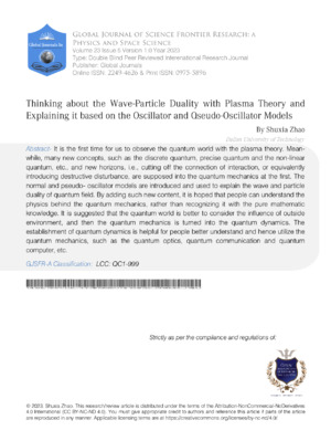\tag {74} $$ This is due to the definition of hyperbolic cosine function, $\cosh (x) = \frac{\exp(x) + \exp(-x)}{2}$. At proper selection of $\beta, \gamma$ values, we can obtain one infinite potential well model when fixing the range of time variable into a very small interval, i.e., $|t| < \varepsilon$. Here, $\varepsilon$ is set as a small quantity, which embodies the instantaneous characteristics of impulse. For instance, we set $\beta = 1, \gamma = 100, \varepsilon = 0.1139$, and obtain the picture of $\mathbf{x}(t)$ in Fig. 1. 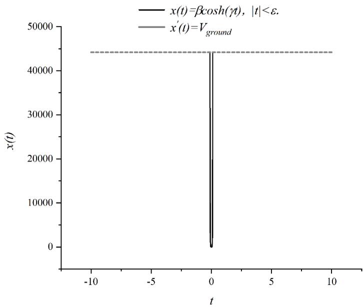 Figure 1: The infinite potential well obtained by the pseudo- oscillator model solution at proper parameter conditions, e.g., $\beta = 1,\gamma = 100,\varepsilon = 0.1139$ It is seen from Fig. 1 the ground of the infinite potential well is determined by the parameter equation, $x'(t) = V_{ground}$. At the present conditions set, $V_{ground} = 44200$. The prime here in the parameter equation, which just represents a different function, is not a derivative operation, the same as in the Figs. 2 and 3. Besides, it is noticed that the infinite potential well obtained by the pseudo- oscillator (at a moment) needs to be observed in the whole-time domain, i.e., it is a truncated solution. This is logic and understandable, since the impulse or quasi- impulse behaviors embody their instantaneous characteristics only when they are seen in the whole time and space. By means of special linear combination, e.g., $y(t) = V_{ground} - x(t)$, we can turn the infinite potential well into an infinitely high potential barrier, as shown in Fig. 2. 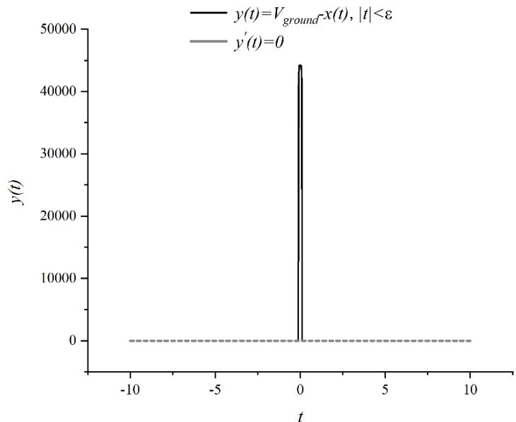 Figure 2: The infinitely high potential barrier obtained from the infinite potential well, by means of the linear combination, $y(t) = V_{\text{ground}} - x(t)$. It is noted that the ground of the potential barrier here is the real ground, i.e., $y'(t) = 0$. Both the infinite potential well and barrier are quasi- impulse behavior, which can be described by an instant force of either pull or push. These behaviors cut off the connection of interaction and can be uniformly defined as one impulse, $\vec{F}_{\text {pull or push }} \delta(t - t_0)$. The potential well and barrier can both shift along the time axis. At the fixed $\beta, \gamma$ values, reform the original function, Eq. (74), into $\mathbf{x}(t - t_0) = \beta \cosh[\gamma (t - t_0)]$, and draw its picture in a new interval, $|t - t_0| < \varepsilon$. Meanwhile, observe it in the whole-time domain and we obtain a shifted potential well in Fig. 3, at the selected parameter value, $t_0 = 5$. Considering the shift property, the Delta function we introduced in the above impulse formula is general, i.e., $\delta(t - t_0)$, other than $\delta(t)$.  Figure 3: The general infinite potential well scheme. It shifts the original function along the time axis to the right side about a distance of $t_0 = 5$. Correspondingly, draw the new potential well in a new infinitely small interval, $|t - t_0| < \varepsilon$, and meanwhile display it in a large time scale, e.g., $t \in [-10,10]$. ## III. INSIGHTS ON THE DEVELOPMENT OF PRESENT QUANTUM MECHANICS FRAMEWORK a) New concepts: discrete quantum, precise quantum, and nonlinear quantum ## i. Loose- bound of particle by potential and discrete quantum In Fig. 4, the one-dimensional infinite potential well with a finite width, which is the classical bound of particle in the present quantum mechanics textbook, is shown. The potential is written in Eq. (75) below. $$ V(x) = \left\{ \begin{array}{ll} 0, & |x| \leq \frac{a}{2}, \\ \infty, & |x| > \frac{a}{2}. \end{array} \right. \tag{75} $$ Substitute the above potential expression into the famous Schrodinger's Equation in Eq. (76) and we get the discrete eigen functions of the particle in Eq. (77), as well as its eigen energy set in Eq. (78). $$ \frac {d ^ {2} \psi (x)}{d x ^ {2}} + \frac {2 m}{\hbar^ {2}} [ E - V (x) ] \psi (x) = 0. \tag {76} $$ $$ \psi_{n}(x) = \left\{ \begin{array}{l} \sqrt{\frac{a}{2}} \sin \frac{n \pi x}{a} \quad (n = 2, 4, 6 \dots), \\ \sqrt{\frac{a}{2}} \cos \frac{n \pi x}{a} \quad (n = 1, 3, 5 \dots). \end{array} \right. \tag{77} $$ $$ E _ {n} = \frac {\hbar^ {2} \pi^ {2} n ^ {2}}{2 m a ^ {2}}, (n = 1, 2, 3, 4, \ldots). (7 8) $$ 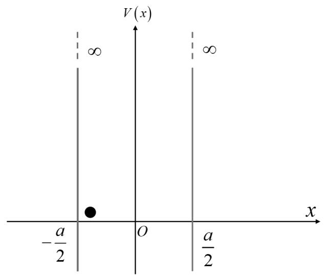 Figure 4: The one-dimensional infinite potential well model, which has a finite width characterized by the parameter, $a$. As seen further, we call the bound of particle by means of infinite potential well with finite width as loose bound, since the particle has limited free space given by the parameter, $a$, and accordingly the solution of Schrodinger equation at the potential of Fig. 1 is called as discrete quantum. ## ii. Equivalent spatial periodicity and the Fourier's series expansion In our understanding, the reason why the solution of Schrodinger equation is discrete is because the space is discretized by the wide potential well. It can be imagined that the whole space is cut into a set of discrete regions by the well, which implicitly represents the spatial periodicity and hence the solution is discretized into the sum of trigonometric functions. This is very like the expansion of a sawtooth wave, which is shown in Fig. 5 and expressed in Eq. (79), into the Fourier series in Eq. (80). The correlation of solving the Schrodinger's equation at bound potential to the Fourier's series expansion, we discovered, inspires us to put forward to the novel concept, discrete quantum. It is noted that at discrete quantum, i.e., in the limited real space, the abstract Hilbert's space is established based on the eigen vectors. As seen next, this is different with the case of tight bound of particle, where only one eigen state is existed. 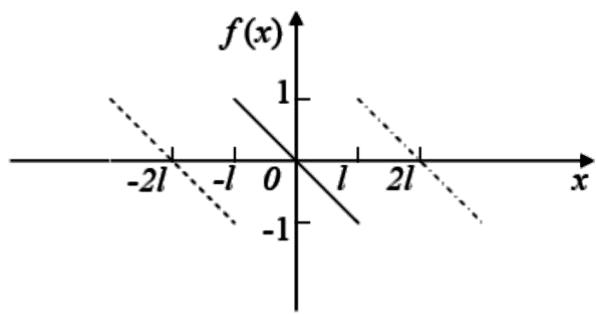 Figure 5: The picture of sawtooth wave, which represents the spatial periodicity. As known, it can be expanded into the Fourier's series, which is essentially discrete and thereby related to the definition of discrete quantum. $$ \mathrm {f} (x) = \left\{ \begin{array}{c} - \frac {x}{l}, - l \leq x \leq l \\ f (x + 2 l) \end{array} \right. \tag {79} $$ $$ \mathrm {f} (x) = \sum_ {n = 1} ^ {\infty} \frac {2 (- 1) ^ {n}}{n \pi} \sin \left(\frac {n \pi x}{l}\right), (- l \leq x \leq l). \tag {80} $$ ## iii. Tight-bound of particle by potential and Single eigen state 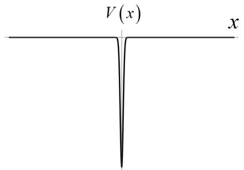 Figure 6: The picture of one-dimensional delta potential well, one example of tight bound of particle. In this section, the one-dimensional delta potential well is plotted in Fig. 6 and written in Eq. (81). It represents the example of tight bound of particle. It is seen from Fig. 6 that the particle is so tightly bounded that it does not have any free space anymore. So, the solution of the Schrodinger's equation of Eq. (82) at the delta potential is only one eigen function, illustrated in Eq. (83). The only eigen energy is given in Eq. (84). Since the single eigen state is obtained at the tight bound of potential, the Hilbert space cannot be constructed. $$ \mathrm {V} (x) = - V _ {0} \delta (x), V _ {0} > 0. \tag {81} $$ $$ \frac {d ^ {2} \psi (x)}{d x ^ {2}} + \frac {2 m}{\hbar^ {2}} [ E + V _ {0} \delta (x) ] \psi (x) = 0. \tag {82} $$ $$ \left\{ \begin{array}{c} \psi (x) = \sqrt{k} e x p (- k | x |) \\ k = \frac{m V _{0}}{\hbar^2} \end{array} \right. \tag{83} $$ $$ \mathrm {E} = - \frac {m V _ {0} {} ^ {2}}{2 \hbar^ {2}}. \tag {84} $$ ## iv. Precise quantum and quasi- soliton We plot, in Fig. 7, the wave function of the Schrodinger's equation at the delta potential bound, i.e., Eq. (83), against the parameter, k, which determines the eigen value, and the soliton solution of KdV equation, i.e., Eq. (67), against the parameter, c, which determines the eigen value as well. It is seen that with the increase of the parameter value, both the wave and soliton functions tend to exhibiting the delta shape, which represents the precise quantum, as we defined, since only one eigen state is existed. Regarding to the similarity between them, the wave function can be called as the quasi- soliton. Note that the soliton shown in Fig. 7(d-f) is a moving soliton, with the constant velocity, c.      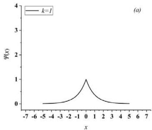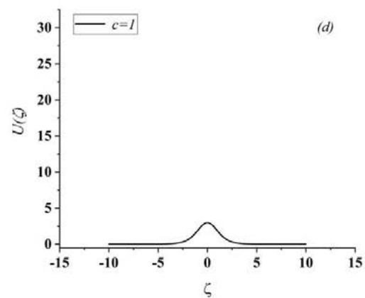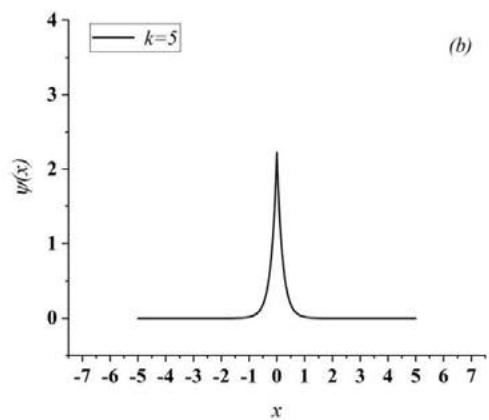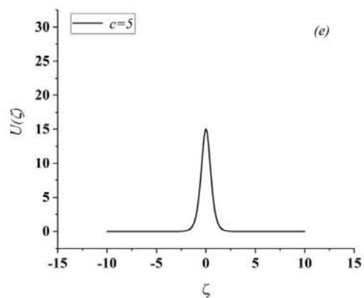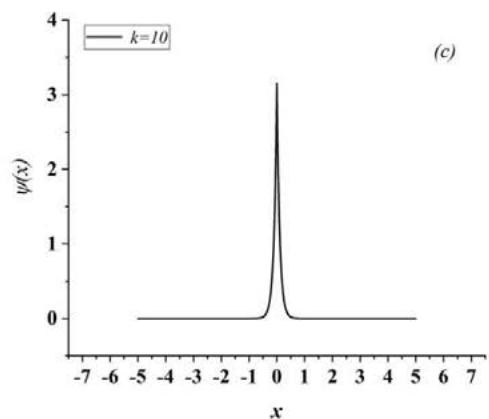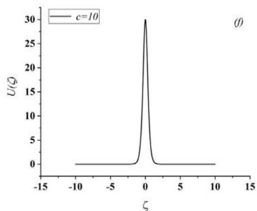 Figure 7: Comparison and the similarity between the solutions of Schrodinger's equation and KdV equation, at the different eigen values, respectively. The former is therefore called as precise quantum, or quasi-soliton, which is determined by the eigen value $k$ or $V_{0}$, more precisely. While the latter is the realistic moving soliton, which is determined by its eigen value, $c$. 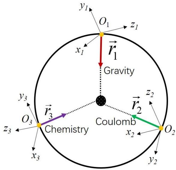## v. Stationary soliton and pseudo-oscillator set In the section, we demonstrate that with a set of pseudo- oscillators, a stationary soliton can be constructed, which behaves more like a wave function of delta type. With the model that consists of a set of pseudo- oscillators, the general reason for the quantization is revealed, e.g., the normal Coulomb force, gravitation force, and the chemical force, etc. The detail of this process is illustrated through the Eqs. (85-91) and the Figs. 8-9. Concretely, in the Eqs. (88-90) set, both the Coulomb and gravitation forces are expanded into the Taylor's series, and furthermore in the Eq. (91) set, each power term of the Taylor's expansion can be treated as a quasi- pseudo- oscillator. Correspondingly, all expanded terms of the two types of force are transformed into a sum of different pseudo- oscillators, which comprises the pseudo- oscillator set. $$ \mathrm {m} \frac {d ^ {2} x}{d t ^ {2}} = k x. \tag {85} $$ $$ \sum_ {i} m _ {i} \frac {d ^ {2} \vec {r _ {l}}}{d t ^ {2}} = k _ {i} \vec {r _ {l}}, \tag {86} $$ $$ \vec {a} _ {\tau i} = 0 \text {(T a n g e t i a l a c c e l e r a t i o n)} \tag {87} $$  $$ \begin{array}{l} \boxed {m _ {1} \frac {d ^ {2} \vec {r} _ {1}}{d t ^ {2}} = k _ {1} \vec {r} _ {1}, \vec {a} _ {\tau , 1} = 0;} \\m _ {2} \frac {d ^ {2} \vec {r} _ {2}}{d t ^ {2}} = k _ {2} \vec {r} _ {2}, \vec {a} _ {\tau , 2} = 0; \\m _ {3} \frac {d ^ {2} \vec {r} _ {3}}{d t ^ {2}} = k _ {3} \vec {r} _ {3}, \vec {a} _ {\tau , 3} = 0; \\\dots \dots \\m _ {i} \frac {d ^ {2} \vec {r} _ {i}}{d t ^ {2}} = k _ {i} \vec {r} _ {i}, \vec {a} _ {\tau , i} = 0. \end{array} $$ Figure 8: The stationary soliton given by the set of pseudo- oscillators 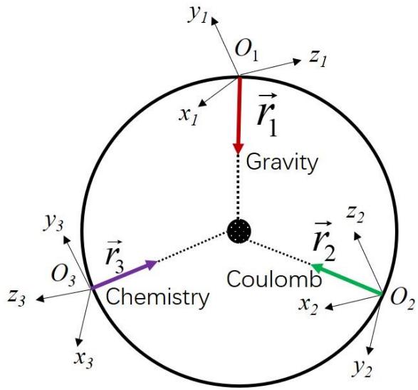 Figure 9: The transformation of Coulomb, gravitation, and chemistry forces into the pseudo- oscillator model $$ \begin{array}{l} \boxed {m _ {1} \frac {d ^ {2} \vec {r} _ {1}}{d t ^ {2}} = \frac {G M m _ {1}}{(\vec {R} - \vec {r} _ {1}) ^ {2}},} \\\boxed {m _ {2} \frac {d ^ {2} \vec {r} _ {2}}{d t ^ {2}} = \frac {q Q}{4 \pi \varepsilon_ {0} (\vec {R} - \vec {r} _ {2}) ^ {2}},} \\\boxed {m _ {3} \frac {d ^ {2} \vec {r} _ {3}}{d t ^ {2}} = k \vec {r} _ {3},} \\\dots \dots . \end{array} $$ $$ \begin{array}{l} \frac {G M m _ {1}}{\left(R - r _ {1}\right) ^ {2}} \sim \frac {A _ {\text{c o n s t}}}{R \left(1 - \frac {r _ {1}}{R}\right) ^ {2}} \sim \frac {1}{R \left(1 - \xi_ {1}\right) ^ {2}}, 0 < \xi_ {1} < 1, (88) \\ \frac {q Q}{4 \pi \varepsilon_ {0} \left(R - r _ {2}\right) ^ {2}} \sim \frac {B _ {\text{c o n s t}}}{R \left(1 - \frac {r _ {2}}{R}\right) ^ {2}} \sim \frac {1}{R \left(1 - \xi_ {2}\right) ^ {2}}, 0 < \xi_ {2} < 1, (89) \\ \frac {1}{(1 - \xi) ^ {2}} = d \left[ \frac {1}{1 - \xi} \right] / d \xi = d (1 + \xi + \xi^ {2} + \xi^ {3} + \dots + \xi^ {n} + \dots) / d \xi (90) \\ = 1 + 2 \xi + 3 \xi^ {2} + \dots + n \xi^ {n - 1} + \dots . \\ \left\{ \begin{array}{c} m \frac {d ^ {2} \xi}{d t ^ {2}} = 2 k \xi , \text{P s e u d o o s c i l l a t o r}, \\ m \frac {d ^ {2} \xi}{d t ^ {2}} = 3 k \xi^ {2}, \text{Q u a s i p s e u d o o s c i l l a t o r}, \\ \dots \\ m \frac {d ^ {2} \xi}{d t ^ {2}} = n k \xi^ {n - 1}, \text{Q u a s i p s e u d o o s c i l l a t o r}. \end{array} \right. (91) \\ \end{array} $$ vi. Homogeneity between the moving soliton and single pseudo- oscillator that re -lates the impulse - $\mathrm{U}(\zeta) = 3c\mathrm{sech}^2\big[(c / 2)^{1 / 2}\zeta \big]\sim c\sim \vec{F}\delta (t - t_0) = \Delta P = mc$ (The momentum law). (92) As seen from the Eq. (92), the moving soliton given by Eq. (67) is determined by the value of parameter, c. Furthermore, the constant velocity of soliton, i.e., the parameter c, is again determined by the impulse given by the single pseudo- oscillator as shown in Fig. 3, through the momentum law. So, the moving soliton and the single pseudo- oscillator that represents the impulse are essentially the same. vii. A pair of conjugate complex solutions for the oscillator and pseudo-oscillator [5, 6] Next, we solve the normal and pseudo- oscillators in the complex domain. In the Eq. (93), the complex solution of normal oscillator is given as a vibration solution. While in the Eq. (94), the complex solution of pseudo- oscillator is a type of instability, as defined in Eq. (95) by means of the planar wave theory of plasma. $$ \left\{ \begin{array}{l} m \frac {d ^ {2} x}{d t ^ {2}} = - k x, \\ \frac {d ^ {2} x}{d t ^ {2}} = - \omega^ {2} x, \\ x = x _ {0} \exp (i \omega t) \end{array} \right. \tag {93} $$ Here, $\omega = \sqrt{\frac{k}{m}}$, and is one real number. $$ \left\{ \begin{array}{c} m \frac{d^2 x}{d t^2} = k x, \\ \frac{d^2 x}{d t^2} = - \omega^{\prime 2} x, \\ x = x_0 \exp (i \omega^{\prime} t). \end{array} \right. \tag{94} $$ Here, $\omega^{\prime} = i\omega$, and is one pure imaginary number. $$ \left\{ \begin{array}{c} x = x _ {0} \exp [ i (k x - \omega t) ], \\I f \omega = \omega_ {r} + i \omega_ {i}, \text {t h e n} \\x = x _ {0} \exp [ i (k x - \omega_ {r} t) ] \exp (\omega_ {i} t). \end{array} \right. \tag{95} $$ Here, $x_0$ is the vibration amplitude and is one real number. In Eq. (95), the planar wave is expressed. Once the angular frequency is a complex number, it is seen that the vibration amplitude will be changed by means of the term, $\exp(\omega_i t)$. And if the imaginary part of angular frequency is positive, the vibration amplitude, $x_0 \exp(\omega_i t)$, diverges. This is called the instability of wave, according to the plasma theory. Moreover, the plasma theory still predicts that once an instability is occurred, the free energy is applied onto the system. Here, in the discussion of the origin of quantization, we propose the free energy is meant either the limited bound potential, which induces the discrete quantum, or the impulse (strong bound potential) that induces the precise quantum. Both the two types of free energy lead the system to form the self-organized structure that dissipates the free energy applied, which might be the deep meaning of quantization. Note that the angular frequency of pseudo- oscillator is a pure and positive imaginary number. It implies none of a little vibration is happened in the pseudo- oscillator, which describes well the meaning of quantization that is against the vibration. viii. Linear and nonlinear quantum dynamics VS. Schrodinger equation and KdV equation (or pseudo oscillator model) In Fig. 10, one discrete eigen sine function versus the time variable, given by the loose bound of potential, is plotted. As seen, it is near the linear regions, represented by the set of red dash lines. This is different with the case of Figs. 1-3 and 7, where the pseudo-oscillator is plotted, which is far away from the linear region. This fact is supported by the function expansion of them, as illustrated in the Eqs. (96, 97). Regarding to this point, the quantum dynamics can be divided into the linear and nonlinear types, which are determined by the Schrodinger Equation and the KdV equation, respectively. As seen from the Sec. (f), the KdV equation is essentially the same as the pseudo- oscillator model that predicts the impulse. Note that the near linear property is also applied to other discrete eigen wave functions, such as the Hermite's polynomial, since they can be expanded into the Fourier's series. 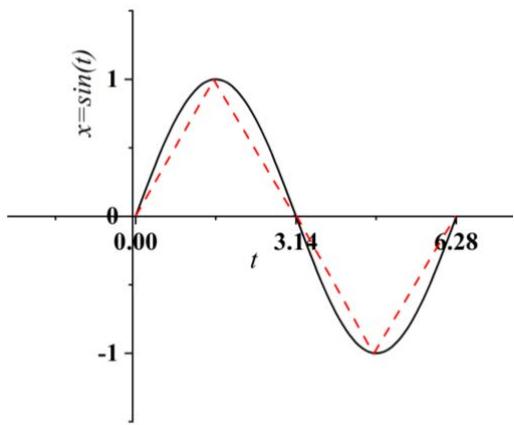 Figure 10: The picture of one discrete eigen sine function. As seen, it is near the linear region, which is represented by the set of red dash lines. $$ \sin (t) = \sum_ {n = 0} ^ {\infty} \frac {(- 1) ^ {n} t ^ {2 n + 1}}{(2 n + 1) !} = t - \frac {t ^ {3}}{3 !} + \frac {t ^ {5}}{5 !} - \frac {t ^ {7}}{7 !} + \dots \tag {96} $$ $$ \left\{ \begin{array}{c} \exp (t) = \sum_{n = 0}^{\infty} \frac{t^{n}}{n!} = 1 + t + \frac{t^{2}}{2!} + \frac{t^{3}}{3!} + \dots (t > 0), \\ \exp (-t) = \sum_{n = 0}^{\infty} \frac{(-t)^{n}}{n!} = 1 - t + \frac{t^{2}}{2!} - \frac{t^{3}}{3!} + \dots (t < 0), \\ \exp (t) = \sum_{n = 0}^{\infty} \frac{|t|^{n}}{n!} = 1 + |t| + \frac{|t|^{2}}{2!} + \frac{|t|^{3}}{3!} + \dots (for\ any\ t). \end{array} \right. \tag{97} $$ ix. New recognition on the bound significance of quantum mechanics, i.e., cutting off the connection We have mentioned this point in the Sec. 2. Here, we want to stress that in all the examples of quantum mechanics listed in the Sec. 3, the bound significance is just to cut off the connection of interaction. ### b) Discussion on the completeness of quantum mechanics i. About the EPR paradox[7] and non-local property The Einstein-Podolsky-Rosen (abbreviated as EPR) paradox discussed the quantum entanglement issue and the non-local property of quantum mechanics. Although it is proven by the Bell inequality experiment and has been applied in the field of quantum communication, the physics behind is not revealed yet. With the idea we presented in this article, i.e., the quantization is originated from the action that cuts off the connection of interaction, the non-local property of quantum entanglement can be easily explained. After the action of truncation, all the interaction is localized into one small region that is characterized by the bound potential and so the space out of this region has no meaning onto the quantum event that is happened inside the region. Here, we are talking about the completeness of quantum mechanics. As seen, it is complete only when we further consider the influence of outside environment. Namely, the quantum mechanics are not always the unitary transformation that is reversible. It can be irreversible, especially when it is measured by introducing disturbance. ii. About one underlying assumption of quantum mechanics, measurement principle In our understanding, when measuring the discrete quantum states, the destructive disturbance is introduced into the Hilbert space. If one eigen state is probed, it means that the particle is trapped into one delta type potential. According to the content of Sec. (3.1c), at delta potential bound, only one eigen state is existed. This means that the Hilbert space must collapse due to the disturbance of this delta potential. As seen, our ideas about the quantization, i.e., destructive disturbance and impulse, underlines the physical basis for the important measurement assumption of quantum mechanics. ## iii. Reconsider the blackbody radiation issue of history By means of the disturbance theory, we can explain well the experiment trends of blackbody radiation. At the low frequency limit, $h\nu \ll kT$, the radiation energy is small and it can be treated as small disturbance to the air molecule in the blackbody cavity. It behaves more like a wave. While at high frequency limit, $h\nu \gg kT$, the radiation is so strong that it now becomes destructive disturbance. The air molecules are now more like transparent to the radiation, and so the radiation can penetrate through the air background and interact directly with the inner boundary of cavity. So, the cavity is now the bound potential to the radiation, and that's why it exhibits the quantum characteristic at high frequency limit. ## IV. CONCLUSION In this article, the pseudo- oscillator model is introduced. Together with the normal oscillator model, the wave and particle duality of quantum mechanics is interpreted, based on the wave theory of plasma, e.g., planar wave, solitary wave and the instability. Many new concepts, such as discrete quantum, precise quantum and nonlinear quantum are introduced, which paves the way of development of quantum mechanics. The disturbance theory is first correlated to the quantum mechanics, which can be classified into the small and destructive types. The origin of quantization is revealed, i.e., by means of introducing the destructive disturbance that discretizes the space and cuts off the connection of interaction, which forms either the loose or tight bound. At loose bound, the discrete eigen states are obtained and the Hilbert space is established, which is essentially the Fourier's series expansion. While at tight bound, the single eigen state is obtained, which can be well described by the concepts such as soliton, whether moving or stationary, and the impulse. In our opinion, the discrete quantum is near linear region, which can be described by the Schrodinger's equation, while the precise quantum is far away from the linear region, which is therefore more suitable to be described by either the KdV equation or the single pseudo- oscillator, i.e., the impulse. In the last, the completeness of quantum mechanics is discussed based on the PRE's paradox and the assumption with respect to the measurement principle of quantum states, through our new opinion on the origin of quantization, i.e., cutting off the connection of interaction or, equivalently, introducing destructive disturbance. ### ACKNOWLEDGEMENT The author (female) is grateful to the young researcher, Dr. Jiasen Jin, for the useful discussion with him when she was attending one lecture of him, quantum mechanics. #### Data availability statement Data available on request from the authors. Conflict of interest The author has no conflicts to disclose.

Generating HTML Viewer...