Atmospheric natural disasters can have their damage mitigated if meteorological alerts are disseminated on time. Among the ways to get data related to weather conditions are the use of atmospheric profilers and numerical models. Such resources can be used for studies related to the surface layer, which covers a range from 20 to 200 meters below the low troposphere. In order to make atmospheric experiments achievable, without great financial expenditure, a low-cost atmospheric profiler was developed together with the Laboratory of Monitoring and Numerical Modeling of Climate Systems (LAMMOC) of the Federal Fluminense University (UFF), to be on board a drone and based on prototyping with Arduino, which had as sensors the DHT22 for measuring temperature and relative humidity and the BMP280 for measuring atmospheric pressure.
## I. INTRODUCTION
From a perspective related to environmental management and about natural disasters, it is necessary to understand that they are the result of extreme or intense natural phenomena, which cause
Author C: Navy Hydrography Center - Brazilian Navy - Niterói 24048-900, Brazil.
social impacts and are mainly characterized by their triggering phenomenon (TOBIN & MONTZ, 1997).
According to the National Civil Defense Policy (PNDEC), disasters are the "result of adverse events on a vulnerable ecosystem, causing human, material and/or environmental damage and consequent economic and social damage" (BRASÍLIA, 2007). The PNDEC also classifies disasters into three types: natural, human-made, and mixed. In this regard, Marcelino (2007) and Castro (1998) point out that most natural disasters would be considered mixed if only this criterion were considered.
According to the 2015 Global Assessment Report (GAR15), prepared by the United Nations Office for Disaster Risk Reduction (UNISDR), annual losses between US$ 250 to 300 billion occur worldwide due to natural disasters, and, with a global investment in prevention, a reduction of up to 20% of these values may occur (GAR, 2015).
The investigation of the thermodynamic mechanisms enables a quick identification of the chances of convective activities developing in a short period, causing storms. In this context, obtaining vertical profiles of the atmosphere through soundings is important for the prognosis of meteorological phenomena such as cloud formation, fog, precipitation, or snow, as well as for investigating atmospheric instability indices (GASPARETTO, 2011).
The surface layer has a thickness that varies between 20 and 200 meters closest to the surface, so that, in this layer, frictional drag, heat conduction and surface evaporation cause substantial variations as a function of height in the temperature, humidity and wind. The behavior of the temperature in this layer varies according to the daily cycle, so that it is common to observe a thermal inversion for the night period. As for turbulent flows, they are relatively uniform with height increments (STULL, 2017).
In addition to knowledge of the thermodynamic conditions of the atmosphere, the use of numerical weather forecast models is also important for making the prognosis of atmospheric phenomena, to be a way to enable the issuance of meteorological alerts (LIRA & CATALDI, 2016). Among such models is the Weather Research and Forecasting (WRF), which can
make forecasts of weather conditions for various levels of the atmosphere, among which is the surface layer (BARCELLOS & CATALDI, 2020).
Thus, in this work the developed atmospheric profiler was embedded in a drone, generating vertical atmospheric profiles in the surface layer, enabling a comparative analysis between these profiles and those obtained through numerical modeling. This led to an assessment of how this approach might be relevant to operational meteorology and data assimilation.
## II. LOW-COST INSTRUMENTATION INITIATIVES
To analyze the characteristics of this layer, atmospheric soundings can be conducted with low-cost sensors attached to a drone together with vertical profiles generated by numerical modeling, so that the results of one can be qualitatively evaluated as a function of the other.
About the use of drones for work and experiments, their application has proved to be very wide. Darynova et al. (2023) applied several controlled methane releases on an environment test platform. A methane-detecting drone and five ground-sensors recorded the methane concentration simultaneously. The hybrid approach, which evaluated both drone and stationary measurements achieved the highest coefficient of determination and the lowest relative error between the reported and model estimated flow rates.
Lee et al. (2022) measured vertically concentrations of particulate matter 2.5 (PM 2.5), black carbon and ozone using a drone in a high-polluted area in South Korea. They found that the concentration of PM 2.5 and black carbon showed minor concentration changes vertically up to 70 meters from the ground and decreased with height over 70 meters. The ozone concentration increased with height up to 30 meters above the surface and increased slowly thereafter.
Järvi et al. (2023) experimentally evaluated the spatial variability of air pollutant concentrations using observations from a mobile laboratory and a drone. They observed that both mean flow and turbulent fluctuations need to be considered when pollutant dispersion and concentrations are examined, and thermal turbulence has strong impact particularly on the formation of aerosol particle hotspots in winter. They also noticed that prediction equations for vertical pollutant decay in a wide street canyon were developed, and the vertical decay was mostly controlled by seasonal variations in air temperature over mean flow and turbulent processes.
Burgués et al. (2022) performed a drone-based system equipped with a lightweight electronic smell sensor for the prediction of odor concentration in a wastewater treatment plant. The accuracy of the odour
predictions by the developed prototype was benchmarked against dynamic olfactometry. They demonstrate that training machine learning algorithms with dynamic sensor signals measured in flight conditions leads to better performance than the traditional approach of using steady-state signals measured in the lab via controlled exposures to odour bags. The comparison of the electronic smell sensor predictions with dynamic olfactometry measurements indicates a negligible bias between the two measurement techniques.
Chang et al. (2018) exploited a novel sampling vehicle, a multi-rotor drone carrying a remote-controlled whole air sampling device, to collect aerial samples with high sample integrity and preservation conditions. An array of 106 volatile organic compounds were analyzed and compared between the aerial samples and the ground-level samples in pairs to inspect for vertical mixing of the trace gases at a coastal location. The study demonstrates that detailed compositions of waste gases can now be easily obtained with superior data quality with the availability of coupling near-surface aerial sampling with laboratory analysis.
Vytovtov et al. (2023) demonstrated how unmanned aerial systems are actively used to provide oil pipelines monitoring, proposed its scientific basis for detecting oil spill accidents formulating the main technical aircraft characteristics applicable for these purposes are formulated and determined the optimal conditions for drone monitoring.
Masic et al. (2021) conducted an experiment in which a robust six-propeller experimental drone was used to launch temperature and suspended particulate matter sensors. In this work, the elements involved in the measurement were placed over the drone hull to avoid the influence of the airflow on the propellers, which was only possible due to the distance of the propellers towards the drone hull.
Karachalios et al. (2021) conducted another experiment with use of a drone with Arduino prototyping to obtain atmospheric data. They proposed that such technology can be especially useful for aviation safety, being able to provide parameters such as temperature, relative humidity, and atmospheric pressure.
Laitinen (2019) attached a Vaisala RD41 probe to the bottom of the DJI Matrice 600 Pro drone. In its case, the propellers were sufficiently far from the sensor. This work aimed to measure temperature and relative humidity. Among its results, it was considered that the airflow coming from the propellers should be a matter to be treated.
Cataldi et al. (2022) developed an equipment based on the Arduino Uno board together with the DHT22 temperature and relative humidity sensor and the BMP280 pressure sensor. This equipment was transported by the DJI Phantom 3 Standard drone with the equipment box fixed to its base. The results pointed
to the suitability of using the DHT22 and BMP280 sensors to measure atmospheric parameters.
It is also useful to list those works that did not necessarily employ drones, but that developed prototypes of sensors of atmospheric parameters.
Oliveira et al. (2016) developed a radiosonde with an Arduino Nano Version 3.0 prototyping board, a BMP180 pressure sensor (previous version of the BMP280 used in this work) and an RF433MHz radiofrequency module, and its radiosonde container it was composed of polystyrene and plastic. This project was conceived to take off with a balloon full of helium gas and for the data to be transmitted by telemetry. The results demonstrated the employability of Arduino technology for this purpose.
Sousa et al. (2022) created a radiosonde with an Arduino Uno board (as used in this work), a DHT11 temperature and relative humidity sensor (previous version of the DHT22 used in this work), an RF433MHz radiofrequency module, a GPS module and a Yagi-Uda type antenna with its adapter. It was conceived for the use of a balloon filled with helium gas, with the differential of having a GPS position transmission to make it easy to be found after its return to the ground.
Ribeiro (2022), with an emphasis on anemometry, used an Arduino Uno board and an MPX5100DP differential pressure sensor associated with a Pitot tube to measure air flows. His device was subjected to several air flows in a low-cost wind tunnel, which allowed him to get a sensor calibration equation.
Aware of this, and with the aim of reducing the costs of atmospheric experimentation campaigns, an atmospheric profiler was developed with the Laboratory for Monitoring and Numerical Modeling of Climate Systems (LAMMOC) at the Fluminense Federal University (UFF), based on Arduino prototyping, which is a programmable computing platform based on the ATmega328P microcontroller with an easy maintenance and capable of interacting with its environment (MCROBERTS, 2011, & ARDUINO, 2023), to be used attached to a drone.
These features enable its association with various devices and sensors, among which are the DHT22, which can be used to measure temperature and relative humidity, and the BMP280, which can be used to measure atmospheric pressure.
## III. MATERIALS AND METHODS
Throughout this work, a low-cost atmospheric profiler based on Arduino prototyping was developed, which was submitted to previous tests, and was used to get the vertical profile of the surface layer. The result of using the profiler was compared to simulated profiles generated by the numerical model Weather Research and Forecasting. Therefore, this section is divided into three parts. The first is dedicated to processes involving
the low-cost profiler, the second is dedicated to drone flight tests and atmospheric experiment, and the third is dedicated to the use of WRF as a tool for qualitative verification of the profiler results.
### a) Low-Cost Atmospheric Profiler
The first step of the implementation of a low-cost atmospheric profiler consists of seeking in the general market an electronic and programmable technology. To that matter, it is important to consider low values compared with the best-known radiosondes either for scientific use or for large-scale use for economic purposes.
As previously mentioned, the Arduino Uno board is based on the ATmega328P microcontroller. Precisely because its functionalities suit the objectives of the project in question, as well as because of the low cost not only of its acquisition and repair, but also of the other sensors and accessory devices involved, that this prototyping path was chosen.
For the measurement of temperature and relative humidity of the air, the DHT22 was chosen, as it adapts to the prototyping board, its cost is low and the DHT11 (its previous version) had good employability in the study by Sousa et al. (2022). Furthermore, when comparing technical descriptions, it was found that DHT22 is twice as accurate as its predecessor. For the measurement of atmospheric pressure, as well as for the calculation of height as a function of the measured pressure, the BMP280 was chosen because, considering the same criteria, it adapts to the Arduino Uno board, has a low cost, its predecessor, the BMP180, was successfully used in the work of Oliveira, Amorim and Dereczynski (2016) and, when comparing technical descriptions, it was found that the accuracy of both was similar in relation to the central value, but the uncertainty range of the BMP180 could cause the errors reached even more than double those possible in the range of the BMP280.
As accessory devices, an RTC DS3231 programmable clock, a MicroSD card module (with its respective card), a 9V rechargeable battery and a small rectangular cardboard box with holes on the sides, enveloped in white, were used. Finally, to transport the profiler, it was decided to use the DJI Mavic Air 2 drone.
Once all the elements necessary for the manufacture of the low-cost atmospheric profiler are arranged, the next step consists of assembling it, for subsequent configuration through a programming script. The assembly was established with a breadboard contact matrix and jumper cables, so that its structure can be verified in Figure 1. As for the configuration, it was done in Arduino programming language through an own development environment, called Arduino Integrated Development Environment (Arduino IDE). The data sampling rate chosen for this script was 10 seconds, which was adopted as a function of the drone
operator conducting a controlled drone flight with a constant ascent speed of $0.1 \, \text{m/s}$ (with few occasional variations).
In the test phase, the influence of the descending air from the drone's propellers on the measurements was treated. This treatment was divided into two parts. In the first part, the MPX5100DP differential pressure sensor was installed in the atmospheric profiler to capture the downward airflow from the propellers. The MPX5100DP was able to identify that the propellers were an influencing factor, but a more accurate sensor was needed to measure it. Thus, in the second part, a flight experiment was conducted with the drone and the Akrom KR835 anemometer to decide how far the profiler should be from the propellers to mitigate this influence.
At the end of the processes, the total budget for implementing the low-cost atmospheric profiler was US$
193.33 without the drone and US $2,076.83 with the drone, which can be used indefinitely, against US$ 4,080.48 for launches of conventional radiosondes (considering the set of radiosonde, meteorological balloon, and helium gas for the 4 synoptic times of the day), for which the materials involved are not recovered.
Thus, an atmospheric experiment was conducted in Itaipu, a neighborhood in the city of Niterói, in the State of Rio de Janeiro, up to a maximum height of 400 feet, or approximately 120 meters, in compliance with the provisions of article E94.701, paragraph 2, of Brazilian Special Civil Aviation Regulation No. 94, Amendment No. 2, issued by the National Civil Aviation Agency (BRASÍLIA, 2021).
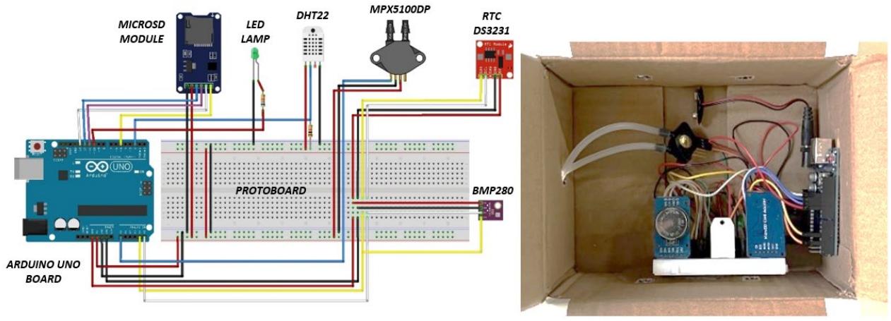 Figure 1: Low-cost atmospheric profiler connections diagram generated in Fritzing software version 0.9.3 (left) and top view of open low-cost atmospheric profiler box (right).
### b) Drone Flight Tests And Atmospheric Experiment
The first time the atmospheric profiler was used happened on August $22^{\text{nd}}$, 2022, as a test, at the Praia Vermelha campus of the Federal Fluminense University (UFF). On that day, the atmospheric profiler box was attached to the base of the DJI Phantom 3 Standard drone by four simple polyamide wires, to distance the atmospheric profiler from the drone.
The second time the atmospheric profiler was used for flight occurred on September $5^{\text{th}}$, 2022, again on a test basis, also at UFF's Praia Vermelha campus. On that day, the atmospheric profiler box was also attached to the base of the DJI Phantom 3 Standard drone by four simple polyamide wires, but quite short this time, to keep the atmospheric profiler and the drone in permanent contact.
After this second test, in which the box was close to the DJI Phantom 3 Standard drone, the influence of the descending air from the drone's propellers was treated on the measurements on January $18^{\text{th}}$, 2023, again at the Praia Vermelha campus of UFF. This study included the use of drones (without an onboard profiler) DJI Phantom 3 Standard and DJI Mavic Air 2, and the Akrom KR835 anemometer. The objective was to measure the speed of this air coming from the propellers to decide on the transport distance between the low-cost atmospheric profiler and the drones.
The third time the profiler was used happened on February $14^{\text{th}}$, 2023, also on a test basis, at UFF's Praia Vermelha campus. On that day, the atmospheric profiler box was attached to a prototype traction cable with 4 thick polyamide wires attached to the rods of the DJI Mavic Air 2 drone's propeller rotors.
The fourth time the profiler was used occurred on March $6^{\text{th}}$, 2023, on a test basis, at UFF's Praia Vermelha campus. On that day, the atmospheric profiler box was attached to the traction cable adapted from its prototype, this time with 1 thick polyamide thread and a carabiner with lock and eye at each end. This cable, in turn, was attached to a device made up of 4 short polyamide fishing wires and a carabiner mounted close to the bases of each drone. On this occasion, the flight stability of both drones was tested. After this test, it was decided to only use the DJI Mavic Air 2 drone to transport the low-cost profiler.
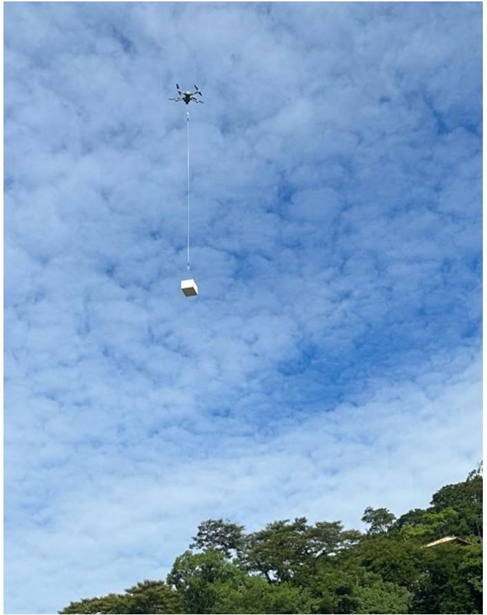
Finally, the fifth time the atmospheric profiler was used for 3 consecutive flights on March $14^{\text{th}}$, 2023, this time to carry out the atmospheric experiment itself, in Itaipu, Rio de Janeiro (as shown in figure 2). On that day, the atmospheric profiler box was attached to the pull cable, and this was attached to the DJI Mavic Air 2 drone.
 Figure 2: Low-cost atmospheric profiler in operation in Itaipu, Rio de Janeiro, on March $14^{\text{th}}$, 2023.
### c) Numerical Model Weather Research and Forecasting
When the atmospheric experimentation was scheduled for March $14^{\text{th}}$, 2023, the Weather Research and Forecasting (WRF) numerical model from the Laboratory for Monitoring and Numerical Modeling of Climate Systems (LAMMOC) was used to generate data for that same day to be count from 00:00 AM GMT until the next subsequent 96 hours. The domain of interest for this round covered the area delimited by points at latitudes $22.50^{\circ}\mathrm{S}$ and $23.13^{\circ}\mathrm{S}$ and longitudes $42.72^{\circ}\mathrm{W}$ and $43.34\mathrm{W}$ (as shown in Figure 3).
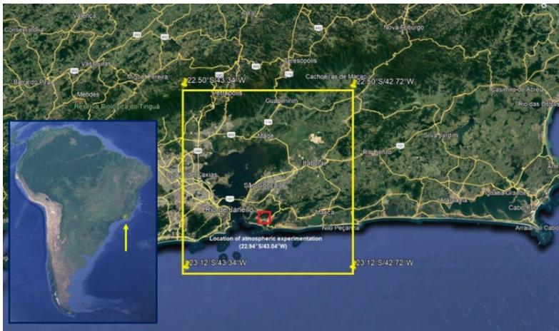 Figure 3: Coverage area of the domain of interest of the March $14^{\text{th}}$, 2023, round of the Weather Research and Forecasting (WRF) numerical model of the Laboratory for Monitoring and Numerical Modeling of Climate Systems (LAMMOC), with emphasis on the location of atmospheric experimentation (in red).
This round generated data for several variables on 34 different vertical levels. For the purposes of this study, data on temperature, relative humidity, atmospheric pressure, and height were used. As the WRF generated more data at higher levels than the atmospheric experimentation campaign with the low-cost profiler, the data of these atmospheric parameters were used for comparative analysis in a range of 995 to 1015 hPa of atmospheric pressure, to cover the entirety of the data observed by the experiment.
More specifically, regarding the configuration of the WRF model, the model grid had 64 points from east to west and 70 points from north to south, totaling 4,480 points. Data from the Global Forecast System (GFS) model were used as initial and boundary conditions, with a periodicity of 21600 seconds (equivalent to 6 hours) between readings. Relating to the parameterizations used, for Micro Physics (mp_physics) the WRF Single-moment 3-class option was used, for Longwave (ra_lw_physics) the RRTM Longwave Scheme option was used, for Shortwave (ra_sw_physics) the Dudhia Shortwave Scheme option was used, for Surface Layer (sf_sfclay_physics) the Revised MM5 Scheme option was used, for Land Surface (sf(surface_physics) the Unified Noah Land Surface Model option was used, and, finally, for Planetary Boundary Layer (bl_pbl_physics) the Yonsei University Scheme (YSU) option was used). The adopted configuration of the WRF numerical model can be seen in Table 1.
Table 1: Numerical Model Weather Research and Forecasting (WRF) - Configuration and parameters.
<table><tr><td colspan="2">time_control</td></tr><tr><td>start (year/month/day/hour/minute/second)</td><td>2023/03/14 00:00:00</td></tr><tr><td>end (year/month/day/hour/minute/second)</td><td>2023/03/18 00:00:00</td></tr><tr><td>intervalSeconds</td><td>21600</td></tr><tr><td colspan="2">domains</td></tr><tr><td>e_we</td><td>64</td></tr><tr><td>e_sn</td><td>70</td></tr><tr><td>e_vert</td><td>35</td></tr><tr><td>dx</td><td>1000</td></tr><tr><td>dy</td><td>1000</td></tr><tr><td colspan="2">physics</td></tr><tr><td>mp_physics</td><td>WRF Single-moment 3-class</td></tr><tr><td>ra_lw_physics</td><td>RRTM Longwave Scheme</td></tr><tr><td>ra_sw_physics</td><td>Dudhia Shortwave Scheme</td></tr><tr><td>sf_sfclay_physics</td><td>Revised MM5 Scheme</td></tr><tr><td>sf(surface_physics</td><td>Unified Noah Land Surface Model</td></tr><tr><td>bl_pbl_physics</td><td>Yonsei University Scheme (YSU)</td></tr></table>
Environmental data modeled by WRF for March 14, 2023, were post-processed with the WRF-Python, which is a package of diagnostic and interpolation routines. For this, an integrated development environment was established in the Windows operating system, which was Anaconda. This environment features the Anaconda Navigator, which is a graphical user interface that allows the user to launch applications and manage "conda" programming packages. Among the applications made available by Anaconda Navigator, JupyterLab was chosen, which is a user interface that offers all the familiar building blocks of the classic Jupyter Notebook application in a flexible World Wide Web (WWW) based format, which makes its employment quite common among data scientists.
## IV. RESULTS AND DISCUSSION
Regarding the results of this work, they are subdivided between the treatment of the influence of the drone's propellers, the surface layer profiles generated by the low-cost atmospheric profiler and the comparison of these profiles with those simulated by the WRF.
### a) Treatment of the Influence of the Drone's Propellers
With the measurement of downward airflow from the propellers by the MPX5100DP, it became evident that this influence should be treated.
Thus, the DJI Mavic Air 2 drone had its downward airflow speed measured for different distances by the Akrom KR835 anemometer (as shown in the Figure 4). With this, it was possible to obtain subsidies for the decision regarding which operating distance should be maintained between the low-cost atmospheric profiler and the drone.
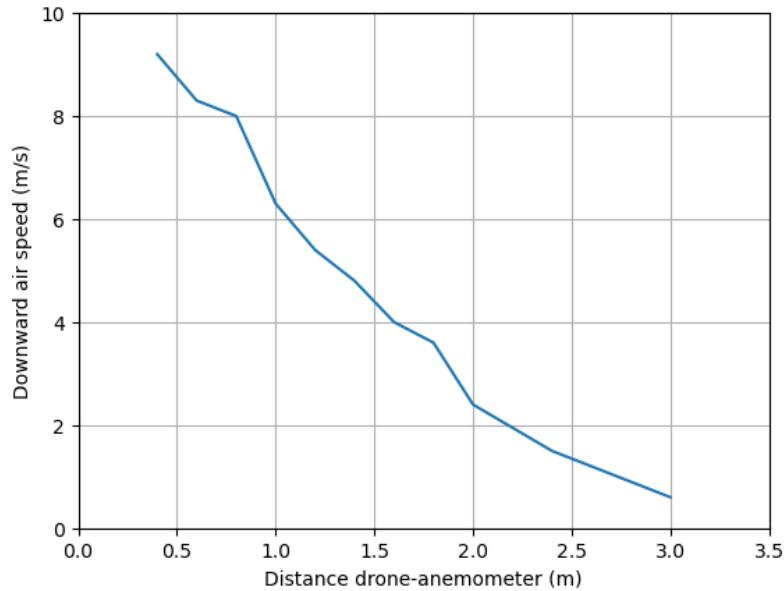 Figure 4: Measurement of the downward air speed from the propellers of the drone DJI Mavic Air 2 as a function of the distance to the Akrom KR835 anemometer (January 18th, 2023).
As a result, it was noticed that the behavior of the airflow speed was inversely proportional to the distance to the anemometer, so that speed became near to zero when this distance reached 3 meters.
In view of this, an attempt was made to use a traction cable that maintained the distance between the profiler and the drone at 3 meters. It was noticed, however, that the profiler had a pendular movement that could endanger the flight safety. This adverse movement was fully mitigated when 2.5 meters was maintained between them. With this solution, it was possible to get low influence of the propellers and satisfactory flight safety at the same time.
When the atmospheric experiment was conducted at Itaipu on March 14th, 2023, it was observed that the profiler remained stable throughout the operation, without any oscillation to disturb the aircraft's steering or decrease the safety of the experiment.
### b) Surface Layer Profiles Generated by the Low-Cost Atmospheric Profiler
In the atmospheric experimentation carried out on March 14, 2023, it was possible to obtain data on temperature, relative humidity, and atmospheric pressure. From the measured pressure it was possible to calculate the height for the measurements. Altogether, 3 vertical flights were performed from 08:03 to 08:14 AM, from 08:19 to 08:26 AM and from 08:46 to 08:54 AM.
About temperature data (as shown in the Figure 5), the first flight registered maximum values just above $28^{\circ}\mathrm{C}$ in the range between 40 and 60 meters high, which corresponds to the range between 1010 and 1008 hPa of atmospheric pressure. The profile data for this flight indicates that there was a thermal inversion from the ground to just over 40 meters in height, which appears to be a residual result of the end of the stable regime of the nocturnal surface layer. From that level upwards, the surface layer behaved like a partially neutral layer.
On the second flight, the temperature values were higher, reaching $28.5^{\circ}\mathrm{C}$ in the range from 80 meters (1006 hPa of atmospheric pressure) to the maximum height. The data from this flight indicates the reduction of the inversion gradient observed in the first flight, presenting a mainly neutral surface layer, with very little vertical temperature variation.
On the third flight, the temperature variation was even greater, registering $30.1^{\circ}\mathrm{C}$ in the first 20 meters of the profile, with values of 1014 to 1012 hPa of atmospheric pressure. Regarding the profile generated for this flight, its data indicate the occurrence of a small inversion in the first 20 meters of height, from where the surface layer becomes neutral up to 60 meters, and, from that level to the top, the profile develops the behavior of an unstable surface layer, with vertical temperature variation approximately logarithmic.
Thus, the data from the three temperature profiles suggested a change in the surface layer regime, which varies from a nocturnal stable layer with slight inversion, passing through a neutral stability layer, until manifesting the beginning of the instability condition.
Regarding relative humidity data (as shown in the Figure 6), on the first flight, values between $65\%$ and $68\%$ were recorded throughout the entire profile. On the second flight, the recorded values were between $66.2\%$ and $70.2\%$. And on the third flight, the relative humidity values began to cover a range from $70.8\%$ close to ground level, around $1014\mathrm{hPa}$ of atmospheric pressure, to a minimum of $61.6\%$ in the range close to 80 meters in height, comprehending values between 1006 and $1004\mathrm{hPa}$ of atmospheric pressure.
The range comprising the relative humidity maximums and minimums in each profile became increasingly wider with the passage of time and consequent increase in temperature, so that the third profile presented the most pronounced variation in the observed values, with a significant increase of humidity close to the soil level, which is consistent with the expected increase in the evaporation rate for the morning period, since the experiment occurred in a grassy field. In addition, the decrease in humidity with height, more markedly at the last measurement time, is another factor associated with the beginning of the instability regime of the surface layer.
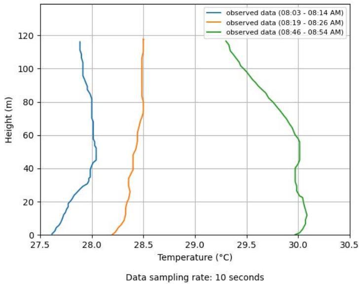 Figure 5: Vertical temperature profiles generated by observed data for Itaipu on March 14th, 2023.
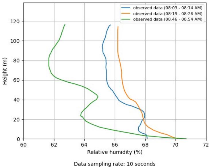 Figure 6: Vertical relative humidity profiles generated by observed data for Itaipu on March 14th, 2023.
Concerning atmospheric pressure data, as the three flights reached a maximum height of 120 meters (with the profiler box reaching 2.5 meters less to avoid propellers influence), all profiles generated by this experiment recorded pressures in the range between 1014.4 and 1001 hPa (as shown in the Figure 7).
About height, it is possible to notice a mainly linear behavior in relation to pressure for the three profiles, with slight oscillations that are probably related to the profiler's ascent speed variations. As previously mentioned, the speed adopted by the profiler remained about $0.1 \, \text{m/s}$, which is low enough to avoid oscillations in flight, but difficult to maintain invariable, as the remote control is very sensitive, being able to vary the speed until $4.0 \, \text{m/s}$ in ascent.
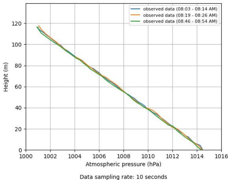 Figure 7: Height profiles as a function of atmospheric pressure generated\\nbymoberved data for Itaipu on March 14th, 2023.
This atmospheric experimentation was significant to demonstrate the applicability of the low-cost profiler with its sensors and its configuration. Moreover, the profiler demonstrated to have thermal inertia small enough to obtain measurements of change in the stability regime of the surface layer. This ability to detect thermal inversion and change in the regime of this layer, from stable, through neutral, to unstable behavior, make it possible for this profiler to be used in studies on atmospheric pollution and nowcasting weather forecast, for example.
### c) Comparison between Observed and Simulated Surface Layer Profiles
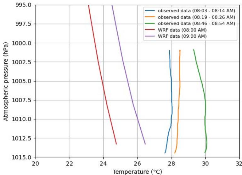
Regarding the comparison between the vertical temperature profiles generated by observed data and by numerical modeling (shown in Figure 8), it is possible to notice that in both cases there was an increase in values as a function of time advance. The observed data are in the range of $27.6^{\circ}\mathrm{C}$ to $30.1^{\circ}\mathrm{C}$, while the modeled data are in the range of $24.8^{\circ}\mathrm{C}$ to $26.4^{\circ}\mathrm{C}$ at the lowest level of the surface layer. This represents a maximum difference of $3.7^{\circ}\mathrm{C}$ between them.
About the detection of thermal inversion and a subtle change in the regime of the surface layer, from stable, through neutral, to unstable, it is only possible to be seen in the observed data, because the modeled data do not have sufficient sensitivity for this purpose.
This fact highlights the importance of this type of experiment, since it could be performed every day (at a very low cost - related only to the electrical energy associated with charging the batteries) and these data could be assimilated by operational models, such as the WRF, increasing its capacity to represent the surface fluxes and, consequently, all the thermal energy transferred to the middle atmosphere.
In the case of the comparison between the vertical profiles of relative humidity generated by observed data and by modeling (shown in Figure 9), the values of the observed data first experience an increase and then suffer a greater reduction, while the modeled values show only the decrease in the considered interval.
It is observed that in the region where it is possible to compare the data, the relative humidity simulated by the WRF was predominantly higher than that observed in the experiment, which may be associated with the underestimation of the air temperature verified in the model simulations at these same levels, which would increase the water vapor retention capacity in the air parcel and, consequently, the relative humidity.
 Data sampling rate: 10 seconds
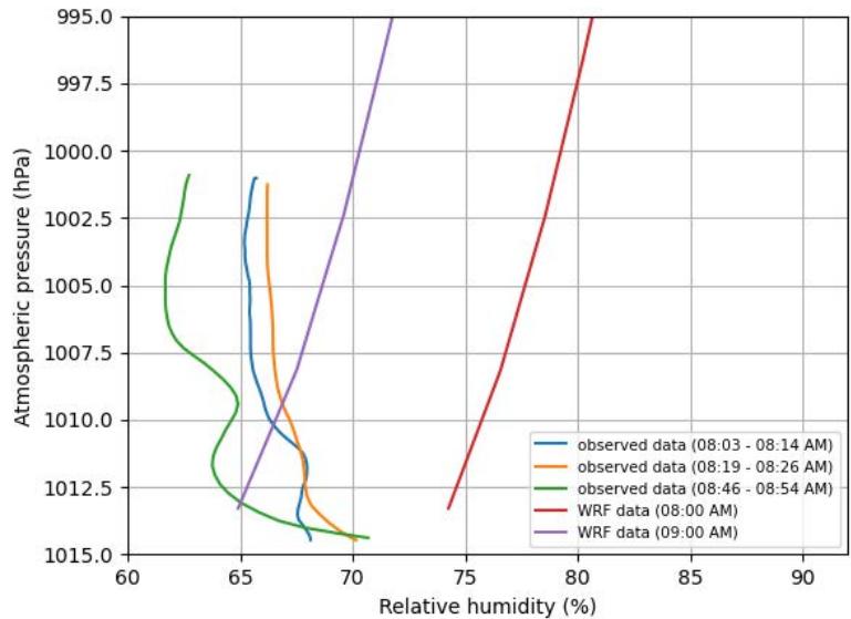 Figure 8: Comparison between vertical temperature profiles generated by observed data and numerical modeling by WRF for Itaipu on March $14^{\text{th}}$, 2023. Data sampling rate: 10 seconds Figure 9: Comparison between vertical relative humidity profiles generated by observed data and numerical modeling by WRF for Itaipu on March $14^{\text{th}}$, 2023.
As for the comparison between the height profiles as a function of atmospheric pressure generated by observed data and by modeling (shown in the Figure 10), there is a correlation between the profiles of their modalities, but a mismatch that varies from 1.6 to $1.8\mathrm{hPa}$ between the profiles generated by observed and modeled data (which are shown superimposed in Figure 9). This may be associated with the difference in atmospheric density between both, since the temperature near the surface simulated by the WRF was about $4^{\circ}\mathrm{C}$ lower than the observed temperature to the same level.
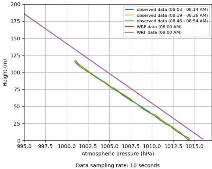 Figure 10: Comparison between height profiles as a function of atmospheric pressure generated by observed data and numerical modeling by WRF for Itaipu on March $14^{\text{th}}$, 2023.
During the course of this study, it was possible to expand the results in relation to the work of Ribeiro (2022), because in addition to anemometry, it was also possible to obtain temperature, humidity and pressure data in a way that was as efficient and economical as his work. Furthermore, the association of the Pitot tube with the MPX5100DP differential pressure sensor made by Ribeiro (2022) could be adapted in this work to reach the perception that drone propellers are an influencing factor for capturing atmospheric data.
The results of the work by Cataldi et al. (2022) pointed to the feasibility of using the DHT22 and BMP280 sensors to measure atmospheric parameters together with the Arduino Uno prototyping board. In light of this, this work not only confirmed the feasibility reported by Cataldi et al. (2022) but also led to the generation of atmospheric vertical profiles, which were analytically compared to numerical modeling profiles, leading to the conclusion that observing data in the atmospheric surface layer with the low-cost profiler contributes positively to a better understanding of the behavior and phenomena of the lower troposphere.
## V. CONCLUSION
As a result of the development of the atmospheric profiler with low-cost technology and sensors, the collected data indicate that it was possible to verify small changes of regime of the surface layer, from its stable, passing through neutral, to unstable behavior. This unfolds the suitability of this profiler to be used in various atmospheric studies, such as atmospheric pollution, calibration of numerical models and nowcasting weather forecast.
It should be noted that this modality of loading sensors, even though they are low cost, on a drone enables successive measurements indefinitely, which is a significant difference in relation to the launch of conventional radiosondes carried by weather balloon due to the high operating costs involved with such launches.
Thus, it is believed that the work fulfilled its purpose, which was to build a methodological approach that allows its replication and improvement for measuring the vertical profile of the atmosphere, initially limited to the surface layer, in addition to having contributed to illustrate the deficiency of atmospheric models in representing surface fluxes, which impacts the predictability of several variables.
Finally, concerning future works, it is recommended that more experiments be performed intensively, at different times of the day, and that other sensors be considered in the prototyping of atmospheric profilers, preferably those that attend guidelines issued by the World Meteorological Organization (WMO). It is also desirable to achieve measurement heights at higher levels, not because of impacts on results, which are satisfactory for the surface layer, but to extend studies beyond this layer. About the profiler's ability to get atmospheric data, it is opportune to study a way to perform measurements of wind speed and direction, considering the type of sensor to be used and the load capacity of the vehicles used to transport it, whether remotely-piloted aircraft or any other.
### ACKNOWLEDGMENTS
We are grateful to Fluminense Federal University (UFF) for academic and financial support, to the Brazilian Navy for providing technical staff, and to the Laboratory for Monitoring and Numerical Modeling of Climate Systems of this university (LAMMOC-UFF) for support related to resource management. We also thank Mr. Daniel Peçanha Simões for his support in designing the low-cost atmospheric profiler prototype.
Generating HTML Viewer...
References
31 Cites in Article
Aosong Eletronics (2017). Table 1: DHT22 sensor testing results for measuring temperature and humidity..
Arduino (2023). Unknown Title.
P Barcellos,M Cataldi (2020). Flash Flood and Extreme Rainfall Forecast through One-Way Coupling of WRF-SMAP Models: Natural Hazards in Rio de Janeiro State.
Ministério Brasília,Da Infraestrutura (2021). Agência Nacional de Aviação Civil.
Brasília (2007). Ministério da Integração Nacional.
Javier Burgués,Silvia Doñate,María Esclapez,Lidia Saúco,Santiago Marco (2022). Characterization of odour emissions in a wastewater treatment plant using a drone-based chemical sensor system.
Adriana Bianchi Azevedo (1998). Avaliação e adequação dos currículos de defesa civil dos cursos de formação e aperfeiçoamento do corpo de bombeiros do rio de janeiro com vista à redução do risco de desastres.
M Cataldi (2022). Atmospheric experimentation with low-cost radiosonde attached to a drone.
Chih-Chung Chang,Chih-Yuan Chang,Jia-Lin Wang,Ming-Ren Lin,Chang-Feng Ou-Yang,Hsiang-Hsu Pan,Yen-Chen Chen (2018). A study of atmospheric mixing of trace gases by aerial sampling with a multi-rotor drone.
Zhuldyz Darynova,Benoit Blanco,Catherine Juery,Ludovic Donnat,Olivier Duclaux (2023). Data assimilation method for quantifying controlled methane releases using a drone and ground-sensors.
Kristin Flemons,Barry Baylis,Aurang Khan,Andrew Kirkpatrick,Ken Whitehead,Shahab Moeini,Allister Schreiber,Stephanie Lapointe,Sara Ashoori,Mishal Arif,Byron Berenger,John Conly,Wade Hawkins (2022). The use of drones for the delivery of diagnostic test kits and medical supplies to remote First Nations communities during Covid-19.
(2015). Disaster risk governance.
P Gasparetto (2011). Relações entre a altura média da camada limite planetária e as condições de instabilidade atmosférica na região metropolitana de Fortaleza -Ceará.
C Graham,I O'connor,L Broderick,M Broderick,O Jensen,H Lally (2022). Drones can reliably, accurately and with high levels of precision, collect large volume water samples and physio-chemical data from lakes.
L Järvi (2023). Determinants of spatial variability of air pollutant concentrations in a street canyon network measured using a mobile laboratory and a drone.
Theodore Karachalios,Dimitris Kanellopoulos,Fotis Lazarinis (2021). Arduino Sensor Integrated Drone for Weather Indices: A Prototype for Pre-flight Preparation.
A Laitinen (2019). Utilization of drones in vertical profile measurements of the atmosphere.
Lee Hwang,H Lee,J (2022). Vertical measurements of roadside air pollutants using a drone.
Clarice Lira,Marcio Cataldi (2016). AVALIAÇÃO DO ENSEMBLE DE PARAMETRIZAÇÕES FÍSICAS DO MODELO MM5 NO EVENTO DE PRECIPITAÇÃO INTENSA OCORRIDO ENTRE OS DIAS 05 E 06 DE ABRIL DE 2010 NO MUNICÍPIO DO RIO DE JANEIRO.
E Marcelino (2007). QUESTIONÁRIO DE DESASTRES NATURAIS NA REGIÃO SUL DO RIO GRANDE DO SUL.
Adnan Masic,Boran Pikula,Dzevad Bibic,Vahidin Hadziabdic,Almir Blazevic (2021). Drone Measurements of Temperature Inversion Characteristics and Particulate Matter Vertical Profiles in Urban Environments.
M Mcroberts,Básico (2011). Unknown Title.
F Oliveira,H Amorim,C Dereczynski (2016). Montagem de uma radiossonda de baixo custo.
Cintia Guimarães Ferreira,Ricardo Tadeu Lopes,Davi Ferreira Oliveira,Thais Maria Pires Do Santos,Olga Oliveira Araújo,Fabiana Dias Fonseca Martins,Gabriela Ribeiro Pereira (2016). Morphological study of defects in laminated joints of composite materials using microCT.
F Ribeiro (2022). Desenvolvimento de sensor embarcado para medição de velocidade do vento.
S Scholz (2023). AED delivery at night -Can drones do the Job? A feasibility study of unmanned aerial systems to transport automated external defibrillators during night-time.
Phablo Sousa,Karla Paula,Daniela Honório,David Silva,Alessandro Martins,Maurício Bolzan (2022). Lançamento de uma sonda atmosférica de baixo custo.
A Christen,R Jassal,T Black,N Grant,I Hawthorne,M Johnson,S-C Lee,M Merkens (2017). Summertime greenhouse gas fluxes from an urban bog undergoing restoration through rewetting.
Tobin,B (1997). Natural hazards: explanation and integration.
A Vytovtov (2023). Scientific Bases Development for Oil Spill Accidents Automated Detection Using Drones.
No ethics committee approval was required for this article type.
Data Availability
Not applicable for this article.
How to Cite This Article
David Christian De Lima Ferreira. 2026. \u201cMeasurement of Vertical Profiles of the Atmospheric Surface Layer With Low-Cost Instrumentation on Board a Drone\u201d. Global Journal of Human-Social Science - B: Geography, Environmental Science & Disaster Management GJHSS-B Volume 23 (GJHSS Volume 23 Issue B5).
Explore published articles in an immersive Augmented Reality environment. Our platform converts research papers into interactive 3D books, allowing readers to view and interact with content using AR and VR compatible devices.
Your published article is automatically converted into a realistic 3D book. Flip through pages and read research papers in a more engaging and interactive format.
Subject: Global Journal of Human-Social Science - B: Geography, Environmental Science & Disaster Management
Authors:
David Christian De Lima Ferreira, Marcio Cataldi, Ivanovich Lache Salcedo, Flávia Rodrigues Pinheiro, Márcio Vinicius Aguiar Soares, Gabriel Ferreira Subtil de Almeida (PhD/Dr. count: 0)
Our website is actively being updated, and changes may occur frequently. Please clear your browser cache if needed. For feedback or error reporting, please email [email protected]
Thank you for connecting with us. We will respond to you shortly.