The turbulences in sticky particles dynamics are described by a class of Markov processes whose the derivatives (velocity fields of turbulence) are backward semi-martingales. The turbulence dynamics is connected to a forced (inhomogeneous) pressure-less gas system.
## I. INTRODUCTION
We are interested in the turbulence of one dimensional fluid flows in one-dimensional sticky dynamics. In [1], the authors considered, in Eulerian coordinates, the velocity field $u$ of fluid particles and a probability field $\mu$ representing their mass or charge distribution. The particles are supposed accelerated between two successive shock times; the dynamics is then governed by a force (measure) field $\nu$. For suitable initial data $(\mu, u)|_{t=0} = (\mu_0, u_0)$ and by discrete approximations, they solved the forced pressureless gas system
$$
\left\{\begin{array}{l}\partial_{t} (\mu) + \partial_{x} (u \mu) = 0\\\partial_{t} (u \mu) + \partial_{x} (u^{2} \mu) = \nu\\\mu_{t} \rightarrow \mu_{0}, u (\cdot , t) \mu_{t} \rightarrow u_{0} \mu_{0} \text{weakly as } t \longrightarrow 0\end{array}\right. \tag{1}
$$
where the force $\nu$ is absolutely continuous, in the space states, with respect to (w.r.t.) $\mu$.
In this paper, we consider non-accelerated fluid particles, so the force of [1] is null and the solution of (1) is thus the one of [2, 8, 3]. In this work, we concentrate our attention on turbines which generate, for (1), a new force whose the support is included in the set of shock (and pure turbulence) sites, in space-time.
Let us first recall the constructions of [2, 8, 3]. They all rely on the sticky particle dynamics which was introduced, at a discrete level, by Zeldovich [9] in order to explain the formation of large structures in the universe. That is a finite number of particles which move with constant velocities while they are not collided. All the shocks are inelastic following the conservation laws of mass and momentum.
At a continuous level, the initial state of particles is given by the support of a non-negative measure $\mu_0$. A particle starts from position $x$ with velocity $u_0(x)$ and mass $\mu_0(\{x\})$. The particles move with constant velocities and masses while not collided. All the shocks are inelastic, following the conservation laws of mass and momentum. In their pioneering work, E et al [8] made this construction when the particles are every where in $\mathbb{R}$, $u_0$ is continuous and the mass of any interval $[a,b]$ is computed with a positive density $f$, i.e. $\mu_0([a,b]) = \int_a^b f(x)\mathrm{d}x$. At time $t$, a particle of position $x(t)$ has the mass $\mu (\{x(t)\},t)$ and the velocity $u(x(t),t)$, the momentum of any interval $[a(t),b(t)]$ is $\int_{a(t)}^{b(t)}u(x,t)\mu (\mathrm{d}x,t)$. The authors then solved (1) with $\nu \equiv 0$.
At the same time and independently, Brenier and Grenier [2] considered the case of particles confined in a in interval $[a,b]$, i.e. $\mu_0([a,b]^c) = 0$. By discretization of $\mu_0$ and using discrete sticky particle dynamics, they solved the scalar conservation law $\partial_t M + \partial_x(A(M)) = 0$ by a weak solution $(M,A)$, the unique which has some entropy condition. As a consequence, the Lebesgue-Stieltjes measure $\partial_x(A(M))$ is absolutely continuous w.r.t. $\partial_xM =: \mu(\cdot,t)$ of Randon-Nicodym derivative a function $u(\cdot,t)$. Then $(\mu,u)$ solves (1) with $\nu \equiv 0$.
In [3], Dermoune and Moutsinga constructed the sticky particles dynamics with an initial mass distribution $\mu_0$, any probability measure, and a initial velocity function $u_0$, any continuous and locally integrable function such that $u_0(x) = o(x)$ as $x \to \infty$. The authors united and generalized previous works of [8, 2] with the arguments that the particles paths define a Markov process $t \mapsto X_t$ solution of the ODE
$$
\mathrm{d}X_{t}=u(X_{t},t)\mathrm{d}t,
$$
and the velocity process $t \mapsto u(X_t, t)$ is a backward martingale. Moreover, $\mu(\cdot, t) = \operatorname{Law}(X_t)$.
In [6, 7], using suitable convex hulls, Moutsinga extended the construction when $\mu_0$ is any non-negative measure and $u_0$ has no positive jump. He gave the description of different kinds of clusters $[\alpha(x,t), \beta(x,t)]$, i.e. the set of all the initial particles $y(0)$ which have the same position $y(t) = x$ at time $t$.
Following the preoccupation of Eyink and Drivas ([4]) about turbulences, Nzissila, Moutsinga and Eyi Obiang [5] defined a turbulent interval as a set $[a,b]$ of initial positions of sticky particles from which rise a turbulence. This means that for all $y\in [a,b]$, the interval $[a,b]$ is the widest among the intervals $[a',b']\ni y$ which have the same position $y + \tau (y)u_{0}(y)$ at their common first shock time $\tau (y)$. The term "turbulence" (instead of "shock") is justified by the description of a degenerated turbulent interval $[a,b] = \{a\}$. In this case, at its mathematical first shock time $\tau (a)$, the particle $a$ does not enter in a real shock but it begins a coagulation process; it enters in a pure turbulence without beginning by a real shock.
At time of turbulence $\tau(a)$, the turbulent interval $[a, b]$ is part of a cluster $[\alpha, \beta] (a, b \in [\alpha, \beta])$. The initial positions $a, b, \alpha, \beta$ are called turbulent particles. The motions of these particles are given by four backward Markov processes, respectively, $Z^1, Z^2, Z^3$ and $Z^4$ solutions of (2) and whose the velocity processes (the derivatives) are semi-martingales.
In this paper, we consider a process $Z$ of more general form than in [5]. The gas system (1) is studied with a force generated at random turbulence time $\gamma = \tau(Z_0)$.
The paper is organized as follows. Section 2 is devoted to the sticky particles model. We recall its definition and the main properties used here. In section 3 we come back to the results of [5] according to the study of turbulence. These results were obtained when the support of $\mu_0$ is an interval (i.e. there is no vacuum of matter). We generalize them to any type of support. The particularity, in presence of vacuum, is that traditional delta-shocks are transformed into butterfly-shocks (like in [3]). Section 4 is devoted to scalar conservation laws from the point of view of turbulent particles. First we give an entropy solution $(N,A)$ with the same flux $A$ as in [2], but with different initial data. Then, in subsection 4.1 we study the gas system. Considering the construction of [5], we define a process of more general form $t\mapsto Z_t = Z_t^1\mathbb{1}_{A^1} + Z_t^2\mathbb{1}_{A^2} + Z_t^3\mathbb{1}_{A^3} + Z_t^4\mathbb{1}_{A^4}$, with the help of any complete system of events $A^1, A^2, A^3, A^4$. A solution of (1), is given by $\mu (\cdot,t)\coloneqq \mathrm{Law}(Z_t)$ and $u(Z_{t},t)\coloneqq \frac{\mathrm{d}Z_{t}}{\mathrm{d}t}$. The force $\nu$ is absolutely continuous w.r.t. the law of the couple $(Z_{\gamma},\gamma)$.
Although this solution is constructed from the sticky particles model, it does not have the properties of [1].
## II. FLOW AND VELOCITY FIELD OF STICKY PARTICLES
### a) The sticky particle dynamics
The definition of one dimensional sticky particle dynamics requires a mass distribution $\mu$, any Radon measure (a measure finite on compact subsets) and a velocity function $u$, any real function such that the couple $(\mu, u)$ satisfies the Negative Jump Condition (NJC) defined in [6]. Precisely, consider the support $\mathcal{S} = \{x \in \mathbb{R}: \mu(x - \varepsilon, x + \varepsilon) > 0, \forall \varepsilon > 0\}$ of $\mu$ and the subsets $\mathcal{S}_{-} = \{x \in \mathbb{R}: \mu(x - \varepsilon, x) > 0\}$, $\mathcal{S}_{+} = \{x \in \mathbb{R}: \mu(x, x + \varepsilon) > 0, \forall \varepsilon > 0\}$. Suppose that $u$ is $\mu$ locally integrable and consider the generalized limits $u^{-}$, $u^{+}$:
$$
u ^ {-} (x) = \lim _ {\varepsilon \rightarrow 0} \sup _ {u (\eta) \in S _ {-}} \frac {\int_ {[ x - \varepsilon , x)} u (\eta) \mu (d \eta)}{\mu [ x - \varepsilon , x)}, \quad \forall x \in S _ {-}, \tag {3}
$$
$$
u ^ {+} (x) = \lim _ {\varepsilon \rightarrow 0} \inf _ {\varepsilon \rightarrow 0} \frac {\int_ {(x , x + \varepsilon ]} u (\eta) \mu (d \eta)}{\mu (x , x + \varepsilon ]}, \quad \forall x \in \mathcal {S} _ {+}. \tag {4}
$$
The Negative Jump Condition requires that
$$
u^{-}(x) \geq u(x) \forall x \in \mathcal{S}_{-}, \quad u(x) \geq u^{+}(x) \forall x \in \mathcal{S}_{+}.
$$
In the whole paper, we mainly use $\mu_0 = \lambda$, the Lebesgue measure. That's why we always suppose that the support $S = \mathbb{R}$.
Considering particles of initial mass distribution $\mu_0$ and of initial velocity function $u_{0}$, their sticky dynamics is defined in [7], when the couple $(\mu_0,u_0)$ satisfies (5) and $x^{-1}u(x)\to 0$ as $|x|\to +\infty$. The dynamics is characterized by a forward flow $(x,s,t)\mapsto \phi_{s,t}(x)$ defined on $\mathbb{R}\times \mathbb{R}_+ \times \mathbb{R}_+$.
### b) Proposition (Forward flow)
For all $x,s,t$..
1. $\phi_{s,s}(x) = x$ and $\phi_{s,t}(\cdot)$ is non-decreasing and continuous.
2. The value $\phi_{s,t}(x)$ is the position after supplementary time $t$ of the particle which occupied the position $x$ at time $s$. More precisely:
$$
\phi_ {s, t} \left(\phi_ {0, s} (y)\right) = \phi_ {0, s + t} (y), \quad \forall y. \tag {6}
$$
3. If $\phi_{0,t}^{-1}(\{x\}) =: [\alpha(x,0,t), \beta(x,0,t)]$ with $\alpha(x,0,t) < \beta(x,0,t)$, then
$$
x = \frac {\int_ {[ \alpha (x , 0 , t) , \beta (x , 0 , t) ]} (a + t u _ {0} (a)) \mathrm {d} \mu_ {0} (a)}{\mu_ {0} ([ \alpha (x , 0 , t) , \beta (x , 0 , t) ])} .
$$
Else
$$
x = \alpha (x, 0, t) + t u _ {0} (\alpha (x, 0, t)) = \beta (x, 0, t) + t u _ {0} (\beta (x, 0, t)).
$$
4. $\beta (x,0,t) + tu_0(\beta (x,0,t))\leq x\leq \alpha (x,0,t) + tu_0(\alpha (x,0,t)).$
If $\mu_0([\alpha (x,0,t),y]) > 0$ and $\mu_0([y,\beta (x,0,t)]) > 0$, then
$$
\frac {\int_ {[ y , \beta (x , 0 , t) ]} (a + t u _ {0} (a)) \mathrm {d} \mu_ {0} (a)}{\mu_ {0} ([ y , \beta (x , 0 , t) ])} \leq x \leq \frac {\int_ {[ \alpha (x , 0 , t) , y ]} (a + t u _ {0} (a)) \mathrm {d} \mu_ {0} (a)}{\mu_ {0} ([ \alpha (x , 0 , t) , y ])}.
$$
5. The function $[0,t] \ni x \longmapsto \phi_{0,s}(\alpha(x,0,t))$ is concave. It is a straight line if and only if $x = \alpha(x,0,t) + tu_0(\alpha(x,0,t))$.
The function $[0,t] \ni x \longmapsto \phi_{0,s}(\alpha(x,0,t))$ is convex. It is a straight line if and only if $x = \beta(x,0,t) + tu_0(\beta(x,0,t))$.
6. For any compact subset $K = [a,b] \times [0,T]$, consider $A_{T} = \alpha (\phi_{s,T}(a),s,T)$, $B_{T} = \beta (\phi_{s,T}(b),s,T)$ and the probability $\mu_s^K = \frac{\mathbf{1}_{[A_T,B_T]}}{\mu_s([A_T,B_T])}\mu_s$. The sticky particle dynamics induced by $(\mu_s^K, u_s)$, during time interval $[0,T]$, is characterized by the restriction of the function $(y,t) \mapsto \phi_{s,t}(y)$ on $[A_T,B_T] \times [0,T]$.
The latter means that the restriction of flow on a compact subset of spacetime does not depend on the whole matter, but only on the restriction of the matter (distribution) on a compact subset of space states.
Remark that if $x = \alpha(x,0,t) + tu_0(\alpha(x,0,t)) = \beta(x,0,t) + tu_0(\beta(x,0,t))$, then the graphs $[0,t] \ni s \mapsto \phi_{0,s}(\alpha(x,0,t))$, $\phi_{0,s}(\beta(x,0,t))$ draw a delta-shock, well known in the literature (Figure 1). Otherwise, these graphs draw a kind of butterfly-shock with foded wings (Figure 2)
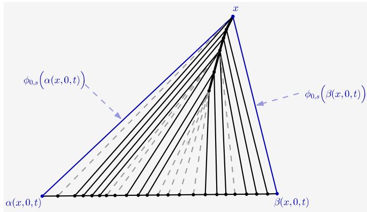 Figure 1: The blue line on the left (resp right) of the middle shock wave represents the trajectory of the particle which started from position
$\alpha(x,0,t)$ (resp $\beta(x,0,t)$ ). It is trajectory $[0,t] \ni s \mapsto \phi_{0,s}(\alpha(x,0,t))$ (resp $[0,t] \ni s \mapsto \phi_{0,s}(\beta(x,0,t)))$
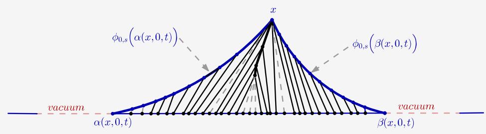 Figure 2: The blue curve on the left (resp right) represent the trajectory of particle which starts at the position
$\alpha(x,0,t)$ (resp $\beta(x,0,t)$ ) which is the trajectory of $[0,t] \ni s \mapsto \phi_{0,s}(\alpha(x,0,t))$ (resp $[0,t] \ni s \mapsto \phi_{0,s}(\beta(x,0,t)))$
What about the velocity?
### c) Proposition (Flow derivative)
1. For all $y, s$, the function $t \mapsto \phi_{s,t}(y)$ has everywhere left hand derivatives. It has everywhere right hand derivatives, except when $\phi_{s,t}^{-1}(\phi_{s,t}(y)) = [a, b]$ with $\mu_s([a, b]) = 0$ and $a < b$. Now and after, the notation $\frac{\partial}{\partial t}\phi_{s,t}(y)$ stands for the right hand derivative.
2. There exists a function $(x,t)\mapsto u_t(x)$ such that $\frac{\partial}{\partial t}\phi_{0,t}(y) = u_t(\phi_{0,t}(y))$ everywhere the right derivative exists.
3. For any compact subset $K = [a,b]\times [0,T]$, consider $A_{T} = \alpha (\phi_{s,T}(a),s,T)$, $B_{T} = \beta (\phi_{s,T}(a),s,T)$ and the probability $\mu_s^K = \frac{\mathbf{1}_{[A_T,B_T]}}{\mu_s([A_T,B_T])}\mu_s$. If the right hand derivative exists for $(x,y)\in K$, the using the conditional expectation under $\mu_s^K$, we have
$$
\frac {\partial}{\partial t} \phi_ {s, t} (y) = \mathbb {E} _ {\mu_ {s} ^ {K}} [ u _ {s} | \phi_ {s, t} (\cdot) = \phi_ {s, t} (y) ]. \tag {7}
$$
We call a cluster at time $t$ all interval of the type $[\alpha(x,0,t), \beta(x,0,t)]$. The last assertion of proposition 2.1 implies an important property on the velocity of a cluster.
### d) Corollary
1. If $[\alpha (x,0,t),\beta (x,0,t)]$ has positive mass, then
$$
u _ {t} (x) = \frac {\int_ {[ \alpha (x , 0 , t) , \beta (x , 0 , t) ]} u _ {0} (a) \mathrm {d} \mu_ {0} (a)}{\mu_ {0} ([ \alpha (x , 0 , t) , \beta (x , 0 , t) ])}.
$$
If $\alpha (x,0,t) = \beta (x,0,t)$, then $u_{t}(x) = u_{0}(\alpha (x,0,t))$.
Else $u_{t}(x)$ is not (well) defined.
#### 2. $u_0(\beta (x,0,t))\leq u_t(x)\leq u_0(\alpha (x,0,t)).$
If $\mu_0([\alpha (x,0,t),y]) > 0$ and $\mu_0([y,\beta (x,0,t)]) > 0$, then
$$
\frac {\int_ {[ y , \beta (x , 0 , t) ]} u _ {0} (a) \mathrm {d} \mu_ {0} (a)}{\mu_ {0} ([ y , \beta (x , 0 , t) ])} \leq u _ {t} (x) \leq \frac {\int_ {[ \alpha (x , 0 , t) , y ]} u _ {0} (a) \mathrm {d} \mu_ {0} (a)}{\mu_ {0} ([ \alpha (x , 0 , t) , y ])}.
$$
3. If $\alpha(x,0,t) \in S_{-}$ (resp. $\beta(x,0,t) \in S_{+}$ ), then $u_{t}^{-}(x) = u_{0}(\alpha(x,0,t))$. (resp. $u_{t}^{+}(x) = u_{0}(\beta(x,0,t))$ ).
4. If $u_0(\alpha(x, 0, t)) = u_t(x)$, then $\mu_0([\alpha(x, 0, t), \beta(x, 0, t)]) = 0$ and $x = \alpha(x, 0, t) + tu_0(\alpha(x, 0, t)) = \beta(x, 0, t) + tu_0(\beta(x, 0, t))$.
5. If $u_0(\beta(x, 0, t)) = u_t(x)$, then $\mu_0([\alpha(x, 0, t), \beta(x, 0, t)] = 0$ and $x = \alpha(x, 0, t) + tu_0(\alpha(x, 0, t)) = \beta(x, 0, t) + tu_0(\beta(x, 0, t))$.
6. For all $t \geq 0$, we have $u_{t}(x) = o(x)$ as $|x| \to +\infty$. For all $t > 0$, if $\alpha(x,0,t) \in S_{-}$ (resp. $\beta(x,0,t) \in S_{+}$ ), then $\lim_{\substack{y \to x \\ y < x}} u_{t}(y) = u_{t}^{-}(x) =$
$$
u_{0}(\alpha (x,0,t)) (\text{resp.}\lim_{\substack{y\to x\\y > x}}u_{t}(y) = u_{t}^{+}(x) = u_{0}(\beta (x,0,t))).
$$
### e) Markov and martingale properties
Let $(\mu_0, u_0)$ be as in theorem 2.1. On abstract measure space $(\Omega, \mathcal{F}, P)$ we define a measurable function $X_0: \Omega \longrightarrow \mathbb{R}$ with image-measure $P \circ X_0^{-1} =$
$\mu_0$. In practice, $(\Omega, \mathcal{F}, P) = (\mathbb{R}, \mathcal{B}(\mathbb{R}), \mu_0)$ and $X_0$ is the identity function. For all $t \geq 0$, we set $X_t = \phi_{0,t}(X_0)$. As a consequence of theorem 2.1, we have the following:
### f) Proposition (Markov and martingale property)
#### 1. $\forall s, t$, we have
$$
X _ {s + t} = \phi_ {s, t} \left(X _ {s}\right) \tag {8}
$$
2. If $u_0$ is $\mu_0$ integrable, then under the measure $\mu_0$ (or $P$ ):
$$
\frac {\mathrm {d}}{\mathrm {d} t} X _ {t} = \mathbb {E} [ u _ {0} (X _ {0}) | X _ {t} ] = u _ {t} (X _ {t}). \tag {9}
$$
Else, for any compact $K = [a,b] \times [0,t + s]$, if $\phi_{0,t + s}(a) \leq X_{t + s} \leq \phi_{0,t + s}(b)$, then under the conditional probability $\mu_0^K$, we get (9).
3. If $u_0$ is $\mu_0$ integrable, then under the measure $\mu_0$ (or $P$ ):
$$
u _ {t + s} (X _ {t + s}) = \mathbb{E} [ u _ {t} (X _ {t}) | \mathcal{F} _ {t + s} ], \quad \text{with} \quad \mathcal{F} _ {t} = \sigma (X _ {u}, u \geq t). \tag{10}
$$
Else, for any compact $K = [a,b] \times [0,t]$, $\phi_{0,t + s}(a) \leq X_{t + s} \leq \phi_{0,t + s}(b)$, then we get (10) under the probability $\mu_0^K$ (or under the conditional probability knowing $\alpha (\phi_{0,t + s}(a), 0, t + s) \leq X_0 \leq \beta (\phi_{0,t + s}(a), 0, t + s)$.
## III. TURBULENCE
In this section, inspired by a preoccupation from [4], we study the sticky particles dynamics from the point of view of turbulence. Generalizing the results of [5], we get a class of Markov processes solution (2). The velocities fields are backward semi-martingales.
### a) Flow, delta-shock and butterfly-shock
In [5], was defined the first turbulence (or shock) time of the particle initial position $a$:
$$
\tau (a) = \inf \left\{t: u ^ {-} \left(\phi_ {0, t} (a), t\right) \neq u ^ {+} \left(\phi_ {0, t} (a), t\right) \right\}. \tag {11}
$$
Let $X_0$ be of image-measure $\mu_0$. Define $\gamma = \tau(X_0)$ and the cluster $[Z_0^3, Z_0^4] = [\alpha(X_\gamma, 0, \gamma), \beta(X_\gamma, 0, \gamma)]$ in which belongs $X_0$ at time $\gamma$. The turbulent interval $[Z_0^1, Z_0^2]$ is defined as the greatest interval containing $X_0$ on which $\tau$ is constant. It was shown in [5] that the velocities of these variables are semi-martingales, when $\mu_0 = \lambda$ the Lebesgue measure. The same result was obtained for the combination $Z_0^5 = Z_0^5\mathbb{1}_A + Z_0^5\mathbb{1}_{A^c}$, with the event $A: {}^n$ the particle enters in the shock from the left". The interesting variable $Z_0^5$ was introduced [4] in order to study the Burgers turbulence.
Our goal is to generalize the results of [5] to any non-negative measure $\mu_0$ and any function $u_{0}$ with negative jumps (w.r.t. $\mu_0$ ). For $i = 1,2,3,4,5$, we consider the process $t\longmapsto Z_t^i = \phi_{0,t}(Z_0^i)$. But one could have other preoccupations than the above event A of [5]. We are led to defined the process of more of more general form $t\longmapsto Z_t = Z_t^1\mathbb{1}_{A^1} + Z_t^2\mathbb{1}_{A^2} + Z_t^3\mathbb{1}_{A^3} + Z_t^4\mathbb{1}_{A^4}$, with the help of any partition $A^1$, $A^2$, $A^3$, $A^4$ of $\Omega$, events of $\sigma(X_0)$. Following the implication the application of the $Z_0^i$ 's, we have fifteen $(2^4 - 1)$ types of processes. (If $A^i = \Omega$; then $Z = Z^i$ ).
## i. Proposition (Random butterfly-shock)
1. Let $Z$ stand independently for $Z^1, Z^2, Z^3$ or $Z^4$.
$$
\forall t, s \geq 0, \quad Z _ {s + t} = \phi_ {s, t} (Z _ {s}), \quad \frac {\mathrm {d}}{\mathrm {d} t} Z _ {t} = u (Z _ {t}, t).
$$
### 2. $\tau(Z_0^1) = \tau(Z_0^2) = \tau(X_0) = \gamma$ and
$$
\forall t \leq \gamma , Z _ {t} ^ {1} = Z _ {0} ^ {1} + t u _ {0} (Z _ {0} ^ {1}) \leq X _ {t} = X _ {0} + t u _ {0} (X _ {0}) \leq Z _ {t} ^ {1} = Z _ {0} ^ {2} + t u _ {0} (Z _ {0} ^ {2}),
$$
$$
\forall t \geq \gamma , X _ {t} = Z _ {t} ^ {1} = Z _ {t} ^ {2} = Z _ {t} ^ {3} = Z _ {t} ^ {4}.
$$
3. $\tau(Z_0^3) \leq \gamma$ and $\tau(Z_0^4) \leq \gamma$.
$[0, \gamma] \ni t \longmapsto Z_t^3$ is concave and $[0, \gamma] \ni t \longmapsto Z_t^3$ is convex.
$$
\forall t \leq \tau \left(Z _ {0} ^ {3}\right), \quad Z _ {t} ^ {3} = Z _ {0} ^ {3} + t u _ {0} \left(Z _ {0} ^ {3}\right)
$$
$$
\forall t \leq \tau (Z_0^4),\quad Z_t^4 = Z_0^4 + t u_0 (Z_0^4);
$$
The segment $[Z_0^1, Z_0^2]$ and the paths $[0, \gamma] \ni t \longmapsto Z_t^1, Z_t^2$ draw a prime delta-shock (so called in [5] because of the first shock time of turbulence).
If $\tau(Z_0^3) = \tau(Z_0^4) = \gamma$, then the paths $[0, \gamma] \ni t \longmapsto Z_t^3$, $Z_t^4$ are linear; and the draw, with the segment $[Z_0^3, Z_0^4]$, delta shock (well known in the literature) (see figure 1).
If $\tau(Z_0^3) < \gamma$ (resp. $\tau(Z_0^4 < \gamma)$ ), then the path $[0, \gamma] \ni \longmapsto Z_t^3$ (resp. $[0, \gamma] \ni \longmapsto Z_t^3$ ) is linear; this can occur o,ly when $Z_0^3 \notin S^-$ (resp. $Z_0^4 \notin S^+$ ). If $\max(\tau(Z_0^3), \tau(Z_0^4)) < \gamma$, then the paths $[0, \gamma] \ni \longmapsto Z_t^3$, $Z_t^3$ draw, not a delta-shock, but butterfly-shock with folded wings (see Figure 3).
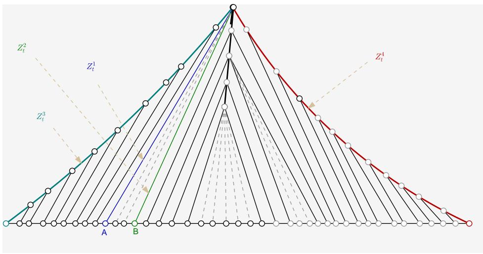 Figure 3: Delta-shock and butterfly-shock
### b) Velocity process as semi-martingale
i. Proposition
1. $t \longmapsto u(Z_t, t) \mathbb{1}_{t < \gamma}$ is bounded variational process adapted to the natural non-increasing filtration $\mathcal{F}^X$ of $X$.
2. For all $t$, $u(Z_{t}, t) = [u(Z_{t}, t) - u_{0}(X_{0})] \mathbb{1}_{t < \gamma} + M_{t}$, with $M_{t} = E\left[u_{0}(X_{0}) | \mathcal{F}_{t}^{X}\right]$. Hence, $t \longmapsto u(Z_{t}, t)$ is a backward càdlàg semi-martingale of $\mathcal{F}^X$.
3. If $\gamma = \tau(Z_0)$, then for all $t$, $u(Z_t, t) = [u_0(Z_0) - M_0] \mathbb{1}_{t < \gamma} + M_t$, with $M_t = E[u_0(X_0) | \mathcal{F}_t^Z]$. Hence, $t \longmapsto u(Z_t, t)$ is a backward càdlàg semi-martingale of $\mathcal{F}^Z$.
4. If $\gamma$ is an optional time of $\mathcal{F}^Z$, then $t \longmapsto u(Z_t, t)$ is a backward càdlàg semi-martingale of the completed filtration $\overline{\mathcal{F}^Z}$. Moreover $t \longmapsto u(Z_t, t) - [u(Z_t, t) - M_\gamma^-] \mathbb{1}_{t < \gamma}$
We recall that for any non-increasing filtration $\mathcal{F}$, the filtration $\overline{\mathcal{F}}$ is defined by $\overline{\mathcal{F}_t} = \sigma (F_t\cup \mathcal{N})$, where $\mathcal{N}$ is the set of negligible events of $\mathcal{F}_0$.
Before the proof, we recall some properties well known in the theory of stochastic processes.
### c) Lemma
Let a process $Z$ be adapted to a non-increasing filtration $\mathcal{G} = (\mathcal{G}_t, t \geq 0)$. Let $\Gamma$ be an optional time with respect to $\mathcal{G}$, i.e. for all $t \geq 0$, the event $\{\Gamma > t\} \in \mathcal{G}_t$. The following holds.
1. The set $\mathcal{G}_{\Gamma}:= \{A \in \mathcal{G}_0: A \cap \{\Gamma > t\} \in \mathcal{G}_t\}$ is a sigma-algebra.
2. If all the paths of $Z$ are either continuous on the right or on the left, then the r.v. $Z_{\Gamma} \mathbb{1}_{\Gamma < \infty}$ is $\mathcal{G}_{\Gamma}$ measurable.
3. Suppose that $\mathcal{G}$ is continuous on the right; that is, for all $t$, $\mathcal{G}_t = \sigma \left( \bigcup_{s > t} \mathcal{G}_s \right)$. If $Z$ is a backward martingale with respect to $\mathcal{G}$, then for all
$t$, the right hand and left hand limits $Z_{t^{+}}$, $Z_{t^{-}}$ exist a.s. Moreover, the process $t \mapsto Z_{(\Gamma \vee t)^{+}} - \Delta_{\Gamma} \mathbb{1}_{\Gamma > t}$ is a backward martingale with respect to the completed filtration $\overline{\mathcal{G}}$, with $\Delta_{\Gamma} = Z_{\Gamma^{+}} - Z_{\Gamma^{-}}$.
### d) Lemma
1. If a process $Z$ is such that $Z_{s + t} = \phi_{s,t}(Z_s)$ for all $t, s \geq 0$, then $\tau(Z_0) \eqqcolon \Gamma$ is an optional time with respect to the natural non-increasing filtration $\mathcal{F}^Z$ of $Z$. Moreover, $\mathcal{F}_0^Z = \mathcal{F}_{\Gamma}^Z$.
2. Suppose that $\{\Gamma \leq t\} \in \mathcal{F}^Z \cap \mathcal{F}^{Z'}$ for some $t \geq 0$. If $Z_t' \mathbb{1}_{\Gamma \leq t} = Z_t \mathbb{1}_{\Gamma \leq t}$, then $\operatorname{E}[F|Z_t'] \mathbb{1}_{\Gamma \leq t} = \operatorname{E}[F|Z_t] \mathbb{1}_{\Gamma \leq t}$ for all integrable r.v. $F$.
The second assertion is satisfied by $(Z, Z') = (X, Z^1)$ and $(Z, Z') = (X, Z^2)$, with $\Gamma = \gamma$. Both $Z^3$ and $Z^4$ satisfy only the first assertion.
Proof. We begin with the first assertion. $u^{-}(\cdot,t),u^{+}(\cdot,t)$ are Borel functions and it is well known that if $u$ is discontinuous in $(Z_{t},t)$, it is also discontinuous in $(Z_{t + s},t + s)$. Then,
$$
\{\Gamma \leq t \} = \{u ^ {-} (Z _ {t}, t) \neq u ^ {+} (Z _ {t}, t) \} \cup [ \{u ^ {-} (Z _ {t}, t) = u ^ {+} (Z _ {t}, t) \} \cap \{\Gamma = t \} ].
$$
Since
$$
\begin{array}{l} \left\{u ^ {-} \left(Z _ {t}, t\right) = u ^ {+} \left(Z _ {t}, t\right) \right\} \cap \left\{\Gamma = t \right\} = \left\{u ^ {-} \left(Z _ {t}, t\right) = u ^ {+} \left(Z _ {t}, t\right) \right\} \cap \\\left[ \bigcap_ {n \geq 1} \left\{u ^ {-} \left(Z _ {t + 1 / n}, t + 1 / n\right) \neq u ^ {+} \left(Z _ {t + 1 / n}, t + 1 / n\right) \right\} \right], \\\end{array}
$$
the proof of the first assertion is done.
Remark that $Z_{t + 1 / n} = \phi_{t,1 / n}(Z_t)$. So $\{\Gamma \leq t\} = Z_t^{-1}(A_t)$, with
$$
A_{t} = \{u^{-}(\cdot,t) \neq u^{+}(\cdot,t)\} \cup \left(\{u^{-}(\cdot,t) = u^{+}(\cdot,t)\} \cap \left[ \bigcap_{n \geq 1} \left\{u^{-}(\phi_{t,1/n},t+1/n) \neq u^{+}(\phi_{t,1/n},t+1/n)\right\} \right]\right) \end{array}
$$
Now we show that $\mathcal{F}_0^Z = \mathcal{F}_{\Gamma}^Z$. First remark that if $\{b\} \neq \phi_{0,t}^{-1}(\phi_{0,t}(b))$, then $\tau(b) \leq t$. Thus for all Borel subsets $B$ and $t \geq 0$, we have $B \cap \{\tau > t\} = \phi_{0,t}^{-1}(\phi_{0,t}(B)) \cap \{\tau > t\}$ and
$$
Z_0^{-1}(B) \cap \{\tau(Z_0) > t\} = Z_t^{-1}(\phi_{0,t}(B)) \cap \{\tau(Z_0) > t\}, \[Z_0^{-1}(B) \cap \{\Gamma > t\} = Z_t^{-1}(\phi_{0,t}(B)) \cap \{\Gamma > t\} \in \mathcal{F}_t^Z.\]
$$
This means that $Z_0^{-1}(B) \in \mathcal{F}_{\Gamma}^Z$.
For the second assertion, since $Z_{t}\mathbb{I}_{\gamma \leq t} = Z_{t}^{\prime}\mathbb{I}_{\Gamma \leq t}$, it is easy to see that $\operatorname {E}[F|Z_t']\mathbb{1}_{\Gamma \leq t}$ is $\sigma (Z_t^\prime)\cap \sigma (Z_t)$ measurable; for all bounded Borel function $h$
$$
\operatorname{E} \big ( h ( Z _ { t } ) \operatorname{E} [ F | Z _ { t } ^ { \prime } ] \mathbb{ 1 } _ { \Gamma \leq t } \big) = \operatorname{E} \big ( h ( Z _ { t } ^ { \prime } ) \operatorname{E} [ F | Z _ { t } ^ { \prime } ] \mathbb{ 1 } _ { \Gamma \leq t } \big) = \operatorname{E} \big ( h ( Z _ { t } ^ { \prime } ) F \mathbb{ 1 } _ { \Gamma \leq t } \big) \
$$
Hence, $\operatorname{E}[F|Z_t']\mathbb{1}_{\Gamma \leq t} = \operatorname{E}[F|Z_t]\mathbb{1}_{\Gamma \leq t}$ a.s.
#### Proof of proposition 3.2
1) The restriction $[0, \gamma[ \ni t \longmapsto u(Z_t, t)$ is monotone. Thus, the process $\mathbb{R}_+ \ni t \longmapsto u(Z_t, t) \mathbb{1}_{t < \gamma}$ is a bounded variational process. It is adapted to $\mathcal{F}^X$ since $\gamma$ is an optional time of this filtration.
2) We have $\mathcal{F}_0^X = \mathcal{F}_\gamma^X$. So for all $t$, the r.v. $u_0(X_0)\mathbb{1}_{t < \gamma}$ is $\mathcal{F}_t^X$ -measurable. Since $\mathcal{F}_t^X = \sigma(X_t)$, we get
$$
\begin{array}{l} u (Z _ {t}, t) \mathbb {1} _ {\gamma \leq t} = u (X _ {t}, t) \mathbb {1} _ {\gamma \leq t} = \underbrace {E [ u _ {0} (X _ {0}) | X _ {t} ]} _ {M _ {t}} \mathbb {1} _ {\gamma \leq t} \\{ = } { M _ { t } - E \left[ u _ { 0 } ( X _ { 0 } ) \mathbb { 1 } _ { t < \gamma } | X _ { t } \right] = M _ { t } - u _ { 0 } ( X _ { 0 } ) \mathbb { 1 } _ { t < \gamma } . } \\\end{array}
$$
Then for all $t$, $u(Z_{t}, t) = [u(Z_{t}, t) - u_{0}(X_{0})] \mathbb{1}_{t < \gamma} + M_{t}$.
3) Same proof as previous, using the fact that $\mathcal{F}_0^Z = \mathcal{F}_\gamma^Z$ and $E\left[u_0(X_0)|X_t\right]\mathbb{1}_{\gamma \leq t} = E\left[u_0(X_0)|Z_t\right]\mathbb{1}_{\gamma \leq t}$ (lemma 3.4)
4) Simple application of lemma 3.3. For all $t$,
$$
u(Z_t,t)\mathbb{1}_{\gamma\leq t} = u(X_t,t)\mathbb{1}_{\gamma\leq t} = E[u_0(X_0)|X_t]\mathbb{1}_{\gamma\leq t} = \underbrace{E[u_0(X_0)|Z_t]}_{M_t}\mathbb{1}_{\gamma\leq t} \= M_{\gamma\lor t} - \Delta_{\gamma}\mathbb{1}_{t<\gamma} - M_{\gamma}^{-}\mathbb{1}_{t<\gamma}
$$
with $\Delta_{\gamma} = M_{\gamma} - M_{\gamma}^{-}$
Remark that assertion 3) is a consequence of 4). Indeed, if $\gamma = \tau(Z_0)$, then $\mathcal{F}_0^Z = \mathcal{F}_\gamma^Z$ (lemma 3.4). So $M_\gamma^-$ and $M_\gamma$ are $\mathcal{F}_\gamma^Z$ measurable and the processes $t \longmapsto M_{\gamma \vee t}$, $M_\gamma \mathbb{1}_{t < \gamma}$, $\Delta_\gamma \mathbb{1}_{t < \gamma}$ are adapted to $\mathcal{F}^Z$. Thus, the process $M_{\gamma \vee t} - \Delta_\gamma \mathbb{1}_{t < \gamma}$ is a backward martingale of $\mathcal{F}^Z$. Hence the process $t \longmapsto u(Z_t, t)$ is a semi-martingale of $\mathcal{F}^Z$.
In fact, $M_{\gamma}\mathbb{1}_{t < \gamma} = M_0\mathbb{1}_{t < \gamma} = M_\gamma^{-}\mathbb{1}_{t < \gamma}$. So the martingale part is $M$.
Now we precise, under more general assumptions, when the velocity of turbulence is a martingale.
### c) Martingales and soft turbulence
In this part, we show that the martingality of the velocity turbulence implies that all mass of any turbulent interval is concentrated in at most one point (single turbulent point). Let $\mathcal{T}$ be the set of turbulent intervals which are not reduced to single points.
### d) Corollary (Turbulence martingales and prime-delta-shocks)
1. The process $t \longmapsto u(Z_t, t)$ is a martingale of $\mathcal{F}^X$ iff a.s. $Z \equiv X$.
2. Suppose that $\gamma$ is an optional time of $\mathcal{F}^Z$ (which is effectively the case when $\mathcal{S}$ is an interval). The process $t \longmapsto u(Z_t, t)$ is a martingale of $\mathcal{F}^X$ iff a.s. $Z_0 = E[X_0|Z_0]$. Furthermore, if $A_i = \Omega$, then a.s. $Z \equiv Z^i \equiv X$.
The following describes the turbulent intervals and clusters when the velocity of their borders are martingales.
### e) Proposition
If $Z_0 = X_0$ a.s., then $\mathcal{T}$ is at most countable and the interior of all turbulent interval is a vacuum.
1. Case $Z \equiv Z^3$ ( $A_3 = \Omega$ ): we have a.e. $Z^3 \equiv Z^1 \equiv X$ and $Z^2 \equiv Z^4$.
$$
\forall [ \alpha , \beta ] \in \mathcal {T}, \mu_ {0} ([ \alpha , \beta ]) = 0; \quad P (Z _ {0} ^ {3} \neq (Z _ {0} ^ {4}) = \sum_ {[ \alpha , \beta ] \in \mathcal {T}} \mu_ {0} (\{\alpha \})
$$
2. Case $Z \equiv Z^4$ ( $A_4 = \Omega$ ): we have a.e. $Z^4 \equiv Z^2 \equiv X$ and $Z^1 \equiv Z^3$.
$$
\forall [ \alpha , \beta ] \in \mathcal {T}, \mu_ {0} ([ \alpha , \beta ]) = 0; \qquad P (Z _ {0} ^ {3} \neq (Z _ {0} ^ {4}) = \sum_ {[ \alpha , \beta ] \in \mathcal {T}} \mu_ {0} (\{\beta \})
$$
any turbulent interval is also a cluster at turbulent time.
3. Case $A_{1} = A_{2} = \emptyset$: we have a.e. $Z^{1}\mathbb{1}_{A_{3}} \equiv Z^{2}\mathbb{1}_{A_{3}}$ and $Z^{2}\mathbb{1}_{A_{4}} \equiv Z^{4}_{A_{4}}$.
$$
\forall [ \alpha , \beta ] \in \mathcal {T}, \mu_ {0} ([ \alpha , \beta ]) = \mu_ {0} (\{\alpha \}) + \mu_ {0} (\{\beta \});
$$
$$
P \left(Z _ {0} ^ {3} \neq \left(Z _ {0} ^ {4}\right) = \sum_ {[ \alpha , \beta ] \in \mathcal {T}} \left[ \mu_ {0} (\{\alpha \}) + \mu_ {0} (\{\beta \}) \right]. \right.
$$
4. Case $Z \equiv Z^1$ ( $A_1 = \Omega$ ): we have a.e. $Z^3 \equiv Z^1 \equiv X$ and $Z^2 \equiv Z^4$.
$$
\forall [ \alpha , \beta ] \in \mathcal {T}, \mu_ {0} ([ \alpha , \beta ]) = 0; \qquad P (Z _ {0} ^ {1} \neq (Z _ {0} ^ {2}) = \sum_ {[ \alpha , \beta ] \in \mathcal {T}} \mu_ {0} (\{\alpha \})
$$
5. Case $Z \equiv Z^2$ ( $A_2 = \Omega$ ): we have a.e. $Z^4 \equiv Z^2 \equiv X$ and $Z^1 \equiv Z^3$.
$$
\forall [ \alpha , \beta ] \in \mathcal {T}, \mu_ {0} ([ \alpha , \beta ]) = 0; \qquad P (Z _ {0} ^ {1} \neq (Z _ {0} ^ {2}) = \sum_ {[ \alpha , \beta ] \in \mathcal {T}} \mu_ {0} (\{\beta \})
$$
Proof: Let us study each semi-martingale.
1. For $Z = Z^3$: A necessary condition is that $E[u_0(Z_0^3)] = E[u(Z_\gamma^3)] = E[u(X_\gamma, \gamma)] = E[u_0(X_0)]$. But $X_\gamma = X_0 + \gamma u_0(X_0) \leq Z_0 + \gamma u_0(Z_0)$ and $Z_0^3\mathbb{1}_{\gamma > 0} = X_0\mathbb{1}_{\gamma > 0}$. Then $\gamma^{-1}(X_0 - Z_0^3)\mathbb{1}_{\gamma > 0} = u_0(Z_0^3) - u_0(X_0) \geq 0$ and $E[\gamma^{-1}(X_0 - Z_0^3)\mathbb{1}_{\gamma > 0}] = 0$. So $X_0 = Z_0^3 = Z_0^1$ a.e. Thus $X \equiv Z^3 \equiv Z^1$ a.e.
In the other hand, we have a.e. $u_0(Z_0^3) \geq u(X_\gamma, \gamma)$ and $E[u_0(Z_0^3) - u(X_\gamma, \gamma)] = 0$. So $u_0(Z_0^3) = u(X_\gamma, \gamma)$ a.e.
Now we show that $Z_0^2 \equiv Z_0^4$. If $Z_0^3 = Z_0^4$, then $Z_0^2 = Z_0^4$. If $Z_0^3 \neq Z_0^4$, then $\exists \alpha < \beta$ s.t. $[Z_0^3, Z_0^4] = [\alpha, \beta]$. If moreover $\mu_0([\alpha, \beta]) = 0$, then $[\alpha, \beta] \in \mathcal{T}$ and $Z_0^2 = Z_0^4 = \beta$. If $\mu_0([\alpha, \beta]) > 0$, then
$$
u _ {0} (\alpha) = u _ {0} (Z _ {0}) = u (X _ {\gamma}, \gamma) = \frac {\int_ {[ \alpha , \beta ]} u _ {0} (x) \mu_ {0} (\mathrm {d} x)}{\mu_ {0} ([ \alpha , \beta ])}.
$$
From corollary 2.3, we get $\mu_0([\alpha, \beta]) = 0$ and $[\alpha, \beta] \in \mathcal{T}$. And again $Z_0^2 = Z_0^4 = \beta$. Thus a.e.: $Z_0^2 = Z_0^4$ and $Z_0^2 \equiv Z_0^4$.
Moreover $\{Z_0^3\neq Z_0^4\} \subset \bigcup_{[\alpha,\beta ]\in \mathcal{T}}\{\alpha \leq X_0\leq \beta \}$. Conversely, if $[\alpha,\beta ]\in$ $\mathcal{T}$, $\exists [\alpha^{\prime},\beta^{\prime}] = [Z_0^3,Z_0^4 ]\supset [\alpha,\beta ]$, with $\mu_0([\alpha ',\beta ']) = 0$. This implies $[\alpha,\beta ] = [\alpha ',\beta ']$. So $\{Z_0^3\neq Z_0^4\} = \bigcup_{[\alpha,\beta ]\in \mathcal{T}}\{\alpha \leq X_0\leq \beta \}$ and $\mu_0([\alpha,\beta ]) = 0$ for all $[\alpha,\beta ]\in \mathcal{T}$. But the set of vacuums is at most countable. So is $\mathcal{T}$. We then get the result $P(\{Z_0^3\neq Z_0^4\})$
2. For $Z = Z^4$: Analogous to previous case.
3. For $Z = Y$: The process $t \mapsto u(Y_t, t)$ is a martingale if only if its bounded variational part vanishes:
$$
a. e \left[ u \left(Y _ {t}, t\right) - u \left(Y _ {\gamma}, \gamma\right) \right] \mathbb {1} _ {t < \gamma}, \forall t.
$$
This equivalent to $u_0(Y_0) = u(Y_t, t) = u(Y_\gamma, \gamma) = u(X_\gamma, \gamma)$ for all $t < \gamma$. Then a.e.
$$
\tau(Y_0) = \gamma,\quad u_0(Y_0) = u(X_\gamma, \gamma),\quad Y_0 + t\gamma u_0(Y_0) = X_0 + t\gamma u_0(X_0).
$$
If $Z_0^3 \neq Z_0^4$, then $\exists \alpha < \beta$ s.t. $[Z_0^3, Z_0^4] = [\alpha, \beta]$ and $Y_0 = \alpha$ or $Y_0 = \beta$. If moreover $\mu_0([\alpha, \beta]) > 0$, then
$$
u _ {0} (\alpha) = u _ {0} (Y _ {0}) = u (X _ {\gamma}, \gamma) = \frac {\int_ {[ \alpha , \beta ]} u _ {0} (x) \mu_ {0} (\mathrm {d} x)}{\mu_ {0} ([ \alpha , \beta ])}.
$$
In this case, if $Y_0 = \alpha$, then from the corollary 2.3, we get $\mu_0([\alpha, \beta]) = 0$ and $Y_0 = Z_0^1 = Z_0^3 = \alpha$. Then $P(Y_0 = \alpha \neq X_0) = \mu_0([\alpha, \beta]) = 0$. In the same way, if $Y_0 = \beta$, we get $Y_0 = Z_0^2 = Z_0^4 = \beta$ and $P(Y_0 = \beta \neq X_0) = \mu_0([\alpha, \beta]) = 0$. In any case, $[\alpha, \beta] \in \mathcal{T}$ and $P(Y_0 \neq X_0, \alpha \leq X_0 \leq \beta) = 0$.
We conclude that $\mathcal{T}$ is at most countable and
$$
\forall [\alpha,\beta] \in \mathcal{T},\\mu_{0}([\alpha,\beta]) = \max(\mu_{0}(\{\alpha\}),\mu_{0}(\{\beta\})) ;
$$
$$
\left\{Z _ {0} ^ {3} \neq Z _ {0} ^ {4} \right\} = \bigcup_ {[ \alpha , \beta ] \in \mathcal {T}} \{\alpha \leq X _ {0} \leq \beta \}
$$
This give the results.
4. For $Z = Z^{1}: E[u_{0}(Z_{0}^{1})] = E[u(Z_{\gamma}^{1}, \gamma)] = E[u_{0}(X_{0})]$. But $u_{0}(Z_{0}^{1}) - u_{0}(X_{0}) = \gamma^{-1}(X_{0} - Z_{0}^{1})\mathbb{1}_{0 < \gamma} \geq 0$. Then a.e.: $Z_{0}^{1} = X_{0}$ and $Z_{0}^{1} \equiv X_{0}$. Furthermore,
$$
\bigl\{Z_{0}^{2}\neq Z_{0}^{1}\bigr \} = \bigcup_{\substack{[\alpha ,\beta ]\in \mathcal{T}\\\alpha < \beta}}\{\alpha \leq X_{0}\leq \beta \}
$$
and for all $[\alpha, \beta] \in \mathcal{T}$, we have
$$
\mu_ {0} ([ \alpha , \beta ]) = P (\alpha < X _ {0} \leq \beta) \leq P (Z _ {0} ^ {1} \neq X _ {0}) = 0.
$$
So $\mathcal{T}$ is at most countable and we get the result for $P(Z_0^2\neq Z_0^1)$.
5. $Z = Z^4$: Analogous to previous case.
Now, we are interested in the conservation laws.
## IV. CONSERVATION LAWS
In this section, we investigate if a process of type of $Z$ can provide solutions to the scalar conservation law
$$
\partial_ {t} M + \partial_ {x} (A (M)) = 0 \tag {12}
$$
and to the pressure-less gas system
$$
\left\{\begin{array}{l}\partial_{t} (\mu) + \partial_{x} (u \mu) = 0\\\partial_{t} (u \mu) + \partial_{x} (u^{2} \mu) = 0\\\mu_{t} \rightarrow \mu_{0}, \qquad u (\cdot , t) \mu_{t} \rightarrow u_{0} \mu_{0} \text{weakly as } t \rightarrow 0\end{array}\right. \tag{13}
$$
It is well known, from the sticky particles model, that the mass distribution $\mu_t$ of the matter and their velocity functions $u(\cdot, t)$ provide a weak solution (in the sense of distributions) to the system (13). The first line of
(13) is usually called conservation law of mass and the second is a conservation law of momentum. Moreover, the couple c.d.f and the momentum function provide an entropy solution to (12). Precisely, $\forall (x,t)\in \mathbb{R}\times \mathbb{R}_{+},$ $M(x,t) = \mu_t([-\infty,x])$
$$
\forall m \in (0, 1), \quad A (m) = \int_ {0} ^ {m} u _ {0} \left(M _ {0} ^ {- 1} (z)\right) d z, \tag {14}
$$
where $M_0 = M(\cdot, 0)$. The equation (12) is conservation law of mass and momentum. Can we have the same thing for the function $N: (x, t) \mapsto P(Z_t \leq x)$ with the same flux (14)?
### a) Proposition
Consider the real function
$$
v _ {0}: a \mapsto \frac {\int_ {Z _ {0} = a} u _ {0} \left(X _ {0}\right) \mathrm {d} P}{P \left(Z _ {0} = a\right)} = E \left[ u _ {0} \left(X _ {0}\right) \mid Z _ {0} = a \right]. \tag {15}
$$
The couple $(N, A)$ is a weak solution of the conservation law (12) if only if $Z$ coincides with the sticky particles process defined from $(N_0, v_0)$.
Before the proof, let us describe what happens in our investigation. From the point of view of the matter, our investigation consists in a change of distributions. We recall that the paths of $Z$ are "extracted" from significant paths of $X$ on which rise turbulences. The extraction procedure redistributes the mass. If $\tau$ is constant on $[a, b]$ and $[\alpha, \beta]$ is the cluster which contains $[a, b]$ at time $\tau(a)$, one of the four particles $\alpha, a, b$ or $\beta$ are extracted. We call them "turbulent particles". All the mass of $[a, b]$ is initially re-affected to these particles. In order to expect the preservation of the conservation law, one can also re-cause the momentum as follows. First remark that each event $A_i$ of section 3.1 is of type " $X_0 \in E_i$ ".
- The mass $\mu_0([a, b] \cap E_3)$ and the momentum $\int_{[a, b] \cap E_3} u_0(x) d\mu_0(x)$ are affected to $\alpha$.
- The mass $\mu_0([a, b] \cap E_1)$ and the momentum $\int_{[a, b] \cap E_1} u_0(x) d\mu_0(x)$ are affected to $a$.
- The mass $\mu_0([a, b] \cap E_2)$ and the momentum $\int_{[a, b] \cap E_2} u_0(x) d\mu_0(x)$ are affected to $b$.
- The mass $\mu_0([a,b]\cap E_4)$ and the momentum $\int_{[a,b]\cap E_4}u_0(x)d\mu_0(x)$ are affected to $\beta$.
- The total mass and total momentum of $\alpha$ and $\beta$ are aggregations of the masses and momenta extracted from turbulent intervals inside $[\alpha, \beta]$. Algorithm: Extraction along the time and aggregation of mass and momentum to $\alpha$ (resp. $\beta$ ) until it is hinted from the left (resp. the right).
The momentum transferred to turbulent particles can also be computed from the flux $A$ (14) and c.d.f $N_0 \coloneqq N(\cdot, 0)$ of $Z_0$. Indeed, the turbulent particles in $[a, b]$ have the momentum
$$
\begin{array}{l} \int_ {\{a \leq Z _ {0} \leq b \}} u _ {0} (X _ {0}) \mathrm {d} P = \int_ {\{a \leq N _ {0} ^ {- 1} \leq b \}} u _ {0} (M _ {0} ^ {- 1} (z)) \mathrm {d} z = \int_ {N _ {0} (a)} ^ {N _ {0} (b)} u _ {0} (M _ {0} ^ {- 1} (z)) \mathrm {d} z \\= A (N _ {0} (b)) - A (N _ {0} (a ^ {-})) \\\end{array}
$$
However, the velocity function induced by this momentum is not the correct one $(u_0)$ for the real dynamics of $Z$. Indeed, each turbulent particle of initial position $a^\prime$ received the mass $P(Z_{0} = a^{\prime})$ and the momentum $\int_{Z_0 = a'}u_0(X_0)\mathrm{d}P$. This induces the velocity
$$
\frac {\int_ {Z _ {0} = a ^ {\prime}} u _ {0} (X _ {0}) \mathrm {d} P}{P (Z _ {0} = a ^ {\prime})} = E [ u _ {0} (X _ {0}) | Z _ {0} = a ^ {\prime} ] = v _ {0} (a ^ {\prime})
$$
So, $A(N_0(b)) - A(N_0(a^-)) = \int_{N_0(a)}^{N_0(b)} u_0(N_0^{-1}(z)) \mathrm{d}z$ is the momentum of another sticky particles dynamics, the one from $(N_0, v_0)$.
Proof of proposition 4.1: Such a weak solution is an entropy solution which is unique once imposed the initial datum $N_0$. Let be the flow constructed from $(N_0, v_0)$ and define $N_t = N(\cdot, t)$. One has $N_t^{-1} = (N_0^{-1}, t)$ for all $t$. Since $Z_t = \phi(Z_0, t)$, one has also $N_t^{-1} = \phi(N_0^{-1}, t)$. So $(\cdot, t) = \phi(\cdot, t)$ on the support of the law of $Z_0$, and one gets $Z_t = (Z_0, t)$ for all $t$.
Now we consider the momentum which corresponds to the dynamics of $Z$, the function $B:(0,1)\ni \mapsto \int_0^m v_0(N_0^{-1}(z))\mathrm{d}Z$. It is also the momentum function of the sticky particles dynamics defined from $(N_0,v_0)$.
### b) Proposition
Suppose that $\gamma = \tau (Z_0)$ a.e. We have
$$
\partial_ {t} N + \partial_ {x} (A (N)) = - \partial_ {x} (C (N, t)) \tag {16}
$$
$$
\partial_{t} N + \partial_{x} (B(N)) = \partial_{x} (D(N,t)) \tag{17}
$$
with, $\forall (m,t)\in (0,1)\times \mathbb{R}_{+}$
$$
C (m, t) = \int_ {0} ^ {m} \Delta_ {0} \left(N _ {0} ^ {- 1} (z)\right) \mathbb {1} _ {t < \tau \left(N _ {0} ^ {- 1} (z)\right)} d z
$$
$$
D(m,t) = \int_0^m \Delta_0 \left(N_0^{-1}(z)\right) \mathbb{1}_{t \geq \tau \left(N_0^{-1}(z)\right)} dz
$$
and $\Delta_0 = u_0 - v_0$
Surprisingly, as shown in the sequel, these results lead to the homogeneous conservation law of the momentum. For all $t$, let $\nu_{t}$ be the distribution of $Z_{t}$, i.e. $\nu_{t}(B) = P(Z_{t} \in B)$ for all Borel set $B$.
### c) Gas system with turbulence force
For all $t$, let $\nu_{t}$ be the distribution of $Z_{t}$, i.e. $\nu_{t}(B) = P(Z_{t} \in B)$ for all Borel set $B$.
### d) Corollary
Let us define $\delta(x, t) = E[\Delta_0(Z_0)|Z_\gamma = x, \gamma = t]$ and consider the law $P_{Z_t,\gamma}$ of $(Z_t, \gamma)$. If $\gamma = \tau(Z_0)$ a.e., then we have
$$
\left\{\begin{array}{l}\partial_{t} (\nu) + \partial_{x} (u \nu) = 0\\\partial_{t} (u \nu) + \partial_{x} (u^{2} \nu) = - \delta P_{Z_{\gamma}, \gamma}\\\nu_{t} \rightarrow \mu_{0}, \quad u (\cdot , t) \nu_{t} \rightarrow u_{0} \nu_{0} \text{weakly as } t \rightarrow 0\end{array}\right.\tag{18}
$$
The couple $(\nu, u)$ is thus a weak solution of a pressure gas system of initial datum is $(\nu_0, u_0)$.
Proof of proposition 4.2: $u(Z_{t}, t) = E\left[v_{0}(Z_{0}) + \Delta_{0}(Z_{0})\mathbb{1}_{t < \tau(Z_{0})}|Z_{t}\right]$. Using $w(Z_{0}, t) \coloneqq v_{0}(Z_{0}) + \Delta_{0}(Z_{0})\mathbb{1}_{t < \tau(Z_{0})}$, we have, for any test function $f$ on $\mathbb{R} \times \mathbb{R}_{+}^{*}$:
$$
\begin{array}{l} \int \int f _ {t} (x, t) N (x, t) \mathrm {d} t \mathrm {d} x = E \int \int f _ {t} (x, t) H (x - Z _ {t}) \mathrm {d} t \mathrm {d} x \\= E \iint f (x, t) u (Z _ {t}, t) \delta_ {Z _ {t}} (\mathrm {d} x) \mathrm {d} t = E \int f (Z _ {t}, t) u (Z _ {t}, t) \mathrm {d} t \\= E \int f (Z _ {t}, t) w (Z _ {0}, t) \mathrm {d} t = - E \int \int f _ {x} (x, t) H (x - Z _ {t}) w (Z _ {0}, t) \mathrm {d} t \mathrm {d} x \\= - \iint f _ {x} (x, t) E [ H (x - Z _ {t}) w (Z _ {0}, t) ] \mathrm {d} t \mathrm {d} x \\\end{array}
$$
and
$$
\begin{array}{l} E \left[ H (x - Z _ {t}) w (Z _ {0}, t) \right] = \int_ {0} ^ {N (x, t)} w (N _ {0} ^ {- 1} (z)) \mathrm {d} z \\= A (N (x, t)) + C (N (x, t), t) = B (N (x, t)) - D (N (x, t), t). \\\end{array}
$$
Proof of corollary 4.3
$$
\begin{array}{l} {E \left[ H (x - Z _ {t}) w (Z _ {0}, t) \right] = E \left[ H (x - Z _ {t}) u (Z _ {t}, t) \right]} = {\int_ {- \infty} ^ {x} u (y, t) \mathrm {d} \nu_ {t} (y),} \\\partial_ {x} \left[ A (N (x, t)) + C (N (x, t), t) \right] = u (x, t) \mathrm {d} \nu_ {t} (x). \\\end{array}
$$
From previous proposition, one gets $\partial_t M + u(x,t)\mathrm{d}\nu_t(x) = 0$. Then, in order to have the first equation of gas system, use the fact that
$$
\partial_ {t} \partial_ {x} M = \partial_ {x} \partial_ {t} M.
$$
It remains the last equation. For any test function $f$ on $\mathbb{R}_+^*$ and any test function $g$ on $\mathbb{R}$,
$$
\begin{array}{l} \int \int f ^ {\prime} (t) g (x) u (x, t) \mathrm{d} \nu_ {t} (x) \mathrm{d} t = E \int f ^ {\prime} (t) g (Z _ {t}) u (Z _ {t}, t) \mathrm{d} t \\= E \int f ^ {\prime} (t) g (Z _ {t}) v _ {0} (Z _ {0}) \mathrm{d} t + E \int f ^ {\prime} (t) g (Z _ {t}) \Delta_ {0} (Z _ {0}) \mathbb{1} _ {t < \tau (Z _ {0})} \mathrm{d} t \\= - E \int f ^ {\prime} (t) g (Z _ {t}) u (Z _ {t}, t) v _ {0} (Z _ {0}) \mathrm{d} t \\+ E \left[ f (\gamma) g (Z _ {\gamma}) \Delta_ {0} (Z _ {0}) \right] - E \int \int f ^ {\prime} (t) g (Z _ {t}) \Delta_ {0} (Z _ {0}) \mathbb{1} _ {t < \tau (Z _ {0})} \mathrm{d} t \\= - E \int f (t) g ^ {\prime} (Z _ {t}) u ^ {2} (Z _ {t}, t) \mathrm{d} t + E \left[ f (\gamma) g (Z _ {\gamma}) \Delta_ {0} (Z _ {0}) \right] \end{array}
$$
This ends the proof.
Generating HTML Viewer...
References
9 Cites in Article
Y Brenier,W Gangbo,G Savare,M Westdickenberg (2013). Sticky particle dynamics with interactions.
Yann Brenier,Emmanuel Grenier (2008). Sticky Particles and Scalar Conservation Laws.
G Drivas,T Eyink (2015). Spontaneous stochasticity and anomalous dissipation for burgers equation.
F Obiang,O Moutsinga,F Nzissila (2021). Backward semimartingale into burgers turbulence.
Octave Moutsinga (2008). Convex hulls, Sticky particle dynamics and Pressure-less gas system.
Octave Moutsinga (2012). Burgers’ equation and the sticky particles model.
Y Rykov,Y Sinai,E Weinan (1996). Generalized variational principles, global weak solutions and behavior with random initial data for systems of conservation laws arising in adhesion particles dynamics.
Y Zeldovich (1970). Gravitational instability, an approximation theory for large density perturbations.
Explore published articles in an immersive Augmented Reality environment. Our platform converts research papers into interactive 3D books, allowing readers to view and interact with content using AR and VR compatible devices.
Your published article is automatically converted into a realistic 3D book. Flip through pages and read research papers in a more engaging and interactive format.
Our website is actively being updated, and changes may occur frequently. Please clear your browser cache if needed. For feedback or error reporting, please email [email protected]
Thank you for connecting with us. We will respond to you shortly.