A New Integral Transform Called Saxena & Gupta Transform and Relation between New Transform and other Integral Transforms

Hemlata Saxena

I. INTRODUCTION
II. PROPERTIES OF SAXENA AND GUPTA TRANSFORM
1. i) Linearity property
2. j) The New transform of Integral
viii) New transform of some elementary function
ix) Compare between New transform and other transform

I. INTRODUCTION

Recently, Integral transformations have played an important role in many fields of science and engineering [1,10,14,15], especially mathematical physics [5], engineering mathematics [16,19], Cryptography [11], image processing [18], mathematical electrodynamics [5] and, a few others, because they have been successfully used in solving many problems in those fields. Integral transforms are one of the most effective tools for solving problems in physics and engineering to obtain a solution for a given differential equation or integral equations by means of inverse transformation. The importance of an integral transforms is that they provide powerful operational methods for solving initial value problems and initial-boundary value problems for linear differential and integral equations.

In view of many interesting properties which make visualization easier, we introduced a new integral transform, termed as "Saxena and Gupta" Transformation. Many of these transforms have been introduced which were extensively used and applied on theory and applications, such as Laplace [6,12,13,17], Fourier [15], Sumudu [4,12], Elzaki [3,8,9], Aboodh [2,19]. Among these, the most widely used is the Laplace transform. Here, a new integral transform is proposed to avoid the complexity of previous transforms.

Definition of New Transform

This transform of a function $f(t)$ defined for all real numbers $t \geq 0$ is the function

The above integral convergent.

Definition of other transform

a) Aboodh transform: The Aboodh transform[2,19] A of a function $f(t)$ for $t$ is greater than or equal to zero given by

b) Laplace transform: The Laplace transform [6],[12],[13],[17] of a function $f(t)$ for $t$ is greater than zero given by

c) Sumudu transform: The Sumudu transform S [4],[12] of a function $f(t)$ for $t$ is greater than or equal to zero given by

d) Elzaki transform: The Elzaki transform $E$ [3],[8],[9] of a function $f(t)$ for $t$ is greater than or equal to zero given by

e) Mahgoub transform: The Mahgoub (Laplace-Carson)M [1] transform of the function $f(t), t \geq 0$ is given by

II. PROPERTIES OF SAXENA AND GUPTA TRANSFORM

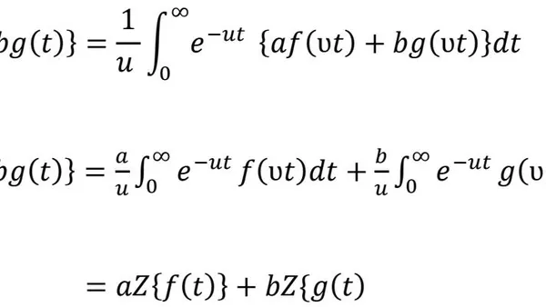
i) Linearity property

Let $Z\{f(t)\}$ denote the New transform of the real function $f$ . Let $f, g$ be a function such that $Z\{f\}$ and $Z\{g\}$ exist.

Proof: Let $a, b \in c$ or $R$ be constant

ii) Shifting property

If the function $\bar{f}(u) = Z\{f\}$ is the transform of the function $f(t)$ then

Proof: $Z\{e^{at}f\} = \frac{1}{v}\int_{0}^{\infty}e^{-t}e^{avt}f(vt)dt$

Let $(1 - a\upsilon)t = x,t = \frac{x}{1 - a\upsilon},dt = \frac{dx}{1 - a\upsilon}$ and put these values in eq.(2.3)

iii) The convolution of two functions

Definition: Assume that $f$ and $g$ are peicewise continuous function, or one of them is dirac's generalized function [7]. The convolution of $f$ and $g$ is a function denoted $f * g$ by and given by the following expression

For every piecewise continuous function $f, g$ and $h$ the following properties hold.

Commutativity $f * g = g * f$
Associativity $f * (g * h) = (f * g) * h$
Distributivity $f * (g + h) = f * g + f * h$
Neutral element $f * 0 = 0$
Identity element $f * 1 = f$

Theorem 1: If the function $f$ and $g$ have well defined transform $Z\{f\}$ and $Z\{g\}$ then

Proof: $Z\{f*g\} = \frac{1}{v}\int_{0}^{\infty}e^{-t}(f*g)(vt)dt$

Let $\lambda = vt$ , $d\lambda = vdt$ put these values in eq.(2.6) then

Put $\gamma = \lambda -\tau$ , $\mathrm{d}\gamma = \mathrm{d}\lambda$ in eq.(2.7) since the variable $\pmb{\tau}$ is constant hence when we integrate with respect to $\pmb{\tau}$ ,we get

Z\{f * g\} = \frac{1}{v^{2}} \int_{0}^\infty \int_{0}^\infty e^{-\frac{\gamma + \tau}{v}} f(\tau) g(\gamma) d\tau d\gamma \quad \dots (2.8)\[\begin{array}{l} = \frac{1}{v^{2}} \int_{0}^\infty e^{-\frac{\gamma}{v}} g(\gamma) d\gamma \cdot \int_{0}^\infty e^{-\frac{\tau}{v}} f(\tau) d\tau \end{array}\]

iv) The New Transform of Derivative and Integral

Derivative property:

If the function $Z\{F\}$ and $Z\{F'\}$ are well defined then

First derivative

Second derivative $Z\{F^{\prime \prime}(t)\} = \frac{1}{v} Z\{f^{\prime}(t)\} -\frac{f^{\prime}(0)}{v^{2}}$

Nth derivative

j) The New transform of Integral

Theorem 2: If the following $Z[f(t)]$ is well defined then

Proof: Suppose that $\mathrm{g}(t - \tau) = 1$ then

vi) The inverse of New transform

Definition: Let the function $\bar{f}(\mathsf{u}) = \bar{Z}\{\mathrm{F}\}$ is the transform of the function $f(t)$ , then $f(t)$ is called the inverse transform $\bar{f}(\mathsf{u})$ and we will write it as

Note: The inverse transform has the linear combination property vii) Solution of some elementary function

1. when $f(t) = 1$ then

2. when $f(t) = t$ then

3. when $f(t) = t^2$ then

4. when $f(t) = t^{n}$ then

5. when $f(t) = e^{at}$ then

6. when $f(t) = \sin at$ then

7. when $f(t) = \cos at$ then

8. when $f(t) = \sinh at$ then

9. when $f(t) = \cosh at$ then

Notes

viii) New transform of some elementary function

Table 1

S.NO.	Function f(t)	New transform Z[f(t)]
1	1	1/v
2	t	1
3	t2	2v
4	tn	un-1Γ(n+1)
5	eat	1/ν(1-av)
6	sinat	a/1+a2v2
7	cosat	1/ν(1+a2v2)
8	sinhat	a/1-a2v2
9	coshat	1/ν(1-a2v2)

ix) Compare between New transform and other transform

Table 5170: Table 2: Sumudu transform and New transform

S.NO.	Function f(t)	Sumudu transform S[f(t)]	New transform Z[f(t)]
1	1	1	1/ν
2	t	ν	1
3	t2	2!/ν2	2ν
4	tn	n!/νn	νn-1/Γ(n+1)
5	eat	1/(1-av)	1/ν(1-av)
6	sinat	av/1+a2v2	a/1+a2v2
7	cosat	1/(1+a2v2)	1/ν(1+a2v2)
8	sinhat	av/1-a2v2	a/1-a2v2
9	coshat	1/(1-a2v2)	1/ν(1-a2v2)

Table 5169: Table 3: Aboodh transform and New transform

S.NO.	Function f(t)	Aboodh transform A[f(t)]	New transform Z[f(t)]
1	1	1/v2	1/ν
2	t	1/v3	1
3	t2	2/v4	2v
4	tn	n!/vn+2	vn-1/Γ (n+1)
5	eat	1/u(u-a)	1/ν (1-av)
6	sinat	a/u(a2+v2)	a/1+a2v2
7	cosat	1/(a2+v2)	1/ν (1+a2v2)
8	sinhat	a/√(v2-a2)	a/1-a2v2
9	coshat	1/(v2-a2)	1/v(1-a2v2)

Table 5168: Table 4: Laplace transform and New transform

S.NO.	Function f(t)	Laplace transform L[f(t)]	New transform Z[f(t)]
1	1	1/u	1/ν
2	t	1/u2	1
3	t2	2!/v3	2v
4	tn	n! s(n+1)	νn-1/Γ(n+1)
5	eat	1/s-a	1/ν(1-av)
6	sinat	a/a2+s2	a/1+a2v2
7	cosat	s/a2+s2	1/ν(1+a2v2)
8	sinhat	a/s2-a2	a/1-a2v2
9	coshat	s/s2-a2	1/ν(1-a2v2)

Table 5167: Table 5: Mahgoub and New transform

S.NO.	Function f(t)	Mahgoub transform M[f(t)]	New transform Z[f(t)]
1	1	1	1/\nu
2	t	1/\nu	1
3	t^2	2! / v^2	2v
4	t^n	\frac{n!}{v^n}	\frac{\upsilon^{n-1}}{\Gamma(n+1)}
5	e^{at}	\frac{u}{(v-a)}	\frac{1}{\upsilon(1-av)}
6	\sinat	\frac{av}{a^2+v^2}	\frac{a}{1+a^2v^2}
7	\cosat	\frac{v^2}{(a^2+v^2)}	\frac{1}{\upsilon(1+a^2v^2)}
8	\sinhat	\frac{av}{v^2-a^2}	\frac{a}{1-a^2v^2}
9	\coshat	\frac{v^2}{(v^2-a^2)}	\frac{1}{\upsilon(1-a^2v^2)}

Table 5166: Table 6: Elzaki and New transform

S.NO.	Function f(t)	Elzaki transform E[f(t)]	New transform Z[f(t)]
1	1	v2	1/v
2	t	v3	1
3	t2	2! v4	2v
4	tn	n! v(n+2)	vn-1/Γ(n+1)
5	eat	v2/(1-av)	1/v (1-av)
6	sinat	av3/1+a2v2	a/1+a2v2
7	cosat	v2/(1+a2v2)	1/v (1+a2v2)
8	sinhat	av3/1-a2v2	a/1-a2v2
9	coshat	v2/1-a2v2	1/v (1-a2v2)

Conclusion: In this paper, we introduce a new integral transform. After that we compare some integral transforms with this new integral transform. It has shows that the new integral transform cover those exiting transforms such as Laplace, Elzaki and Sumudu transform for different values. Also gave properties of new transform and derivatives. Researcher can use this new integral transform for solving ODE, integral equations and fractional differential and integral equations.