## I. INTRODUCTION Atmospheric aerosol is the combination of all condensed-phase materials present in the atmosphere. Aerosol particles play two distinct roles. As a condensed phase material, they have physical functions as absorbers, emitters, and scatters of atmospheric radiation [1]. They also provide favorable surfaces for depositing molecules and/or ions from the fluid in which they are embedded. These atmospheric particles also participate in many processes with climate impact. In addition, they exert a direct and indirect effect on the radiative balance of the atmosphere, acting as condensation nuclei in the hydrological cycle on regional and global scales [2, 3]. According to the latest Intergovernmental Panel on Climate Change reports, atmospheric aerosols are still responsible for one of the greatest uncertainties in understanding their role in climate change [4]. Aerosols, such as sea salt, mineral particles, carbonaceous aerosols, and particles from fauna and flora, can be of natural origin. In addition to natural sources, it is also necessary to consider anthropogenic emissions, which are responsible for a substantial portion of this particulate matter in the atmosphere [5]. They also play a significant role in the hydrological cycle, acting as condensation nuclei [6]. Therefore, its quantification and characterization are essential for understanding the behavior of processes operating in the Earth's atmosphere [7]. Many studies indicate that depending on their type, they can change the rainfall pattern of seasonal systems such as monsoons [8, 9], climate oscillation patterns such as Southern Ring Mode (SAM) [10], and transient systems [7]. Although the number of studies on atmospheric aerosols has increased in recent years, mainly due to the greater availability of data obtained by remote sensing, some areas still need further investigation. For example, as is the case of the study area of this work, which comprises the Metropolitan Region of Rio de Janeiro (MARJ). This region is such a city, situated at a tropical latitude $(\sim 22.8^{\circ}\mathrm{S}, 43.1^{\circ}\mathrm{W})$ over a complex terrain partially covered with rainforest and includes multiple watershed basins feeding the Guanabara Bay. It is the second largest conurbation in Brazil and the second region with the most significant economic importance for the country. Because of its fast development in the past years, it is becoming a region with more than 12 million people. During the last decade, MARJ has undergone several changes in structure and urbanization. A suitable air quality monitoring network for the entire region did not accompany these changes. The main goal of this work is to trace a temporal analysis of aerosols for a region of Rio de Janeiro centered on the MARJ, analyzing its origin and characteristics. In the absence of a conventional observation network, the use of remote sensing and reanalysis data becomes of crucial importance. For this, a set of remote sensing data and reanalysis were used: the Cloud-Aerosol Lidar with Orthogonal Polarization (CALIOP) sensor aboard the Cloud-Aerosol Lidar and Infrared Pathfinder Satellite Observation (CALIPSO) satellite, one of the leading remote observation instruments for the study of aerosols; the reanalysis of the Modern Era Retrospective Analysis Version 2 (MERRA 2), which takes into account various physical processes in which aerosols are involved; simulations made with the Hybrid Single Particle Lagrangian Integrated Trajectory (HYSPLIT), for tracking air masses and understanding from where these air masses that bring these particles; and finally, the Moderate Resolution Imaging Spectroradiometer (MODIS) sensor, with high-resolution products for the study of fires. ## II. METHODS The CALIOP sensor, on board the CALIPSO, is a lidar that generates vertical profiles of the distribution of aerosols and clouds with their respective optical properties [11]. It is the only orbital platform that enables these observations. CALIPSO maintains a near sun-synchronous orbit with an altitude of 705 km, an inclination of $98.2^{\circ}$, and a period of 98.3 minutes, providing a worldwide high-resolution aerosol vertical profiles with a temporal resolution of 16 days. It takes measurements at two different wavelengths, $532\mathrm{nm}$ in the visible spectrum and $1064\mathrm{nm}$ in the near-infrared spectrum. The sensor's accuracy allows measurements at the same point on the earth's surface with a variation of only $10\mathrm{km}$. Therefore, the number of passes in the study area is approximately two per month, one in the ascending and one in the descending orbit. In this study, thirteen years of data from the CALIPSO satellite were used between 2006, the year of the beginning of operations, and 2019, the year chosen before the suspension of activities due to the COVID-19 pandemic, totaling 530 satellite passes. Two products from CALIPSO were used, the Feature Classification Flags, with processing level 1, and the "Aerosol," with processing level 3, following the methodology proposed by [11, 12]. The Feature Classification Flags classify different atmospheric elements in vertical profiles, while the "Aerosol" has variables related to the physical properties of aerosols in vertical layers. The Vertical Feature Mask (VFM) variable was used from the Feature Classification Flags. The VFM decision tree first separates each pixel of the vertical profile as cloud, aerosol, or undetermined. After this initial process, other branches in the decision tree emerge, classifying each cloud type and aerosols. In the next step, only the pixels classified as aerosols were filtered, and finally, the different types of aerosols were separated throughout the database. Classifying aerosol pixels into clean marine, dust, polluted continental, clean continental, polluted dust, and smoke is possible. Smoke and polluted continental are attributed to anthropogenic emissions, while dust, clean continental, and clean marine are from natural emissions. The polluted continental type is a hybrid, a mixture of smoke and dust [12]. As for the Aerosol Optical Depth, the average across the entire atmospheric column was used as the data are arranged in vertical layers. These data have a horizontal and vertical resolution that varies with altitude, as shown in Table 1. Vertically and horizontally, respectively, the resolution up to $8.2\mathrm{km}$ is 30 and $333\mathrm{m}$; between 8.2 and $20\mathrm{km}$, the resolution is 60 and $1000\mathrm{m}$; between 20 and $30\mathrm{km}$, the resolution is 180 and $1667\mathrm{m}$. The present study used version 4.10 of level 2 aerosol products, which substantially improved the aerosol type, lidar algorithms, and rigid quality control [13]. In order to compare and complement the data obtained by the CALIOP sensor, MERRA 2 data were used, a reanalysis with a horizontal resolution of $0.5^{\circ} \times 0.625^{\circ}$ and 72 ETA-hybrid vertical levels. This reanalysis uses version 5.12.4 of the GEOS system for assimilating observed data from the atmosphere and takes into account some essential factors for the study of aerosols, such as the assimilation of observed radiance data and the deposition of aerosols in its simulations [14]. Table 1: Spatial resolutions of the CALIOP sensor for two wavelength- CALIPSO Satellite. <table><tr><td>Altitude (km)</td><td>Horizontal Resolution (km)</td><td>Vertical Resolution (m) (532nm)</td><td>Vertical Resolution (m) (1064nm)</td></tr><tr><td>30.1 to 40.0</td><td>5.0</td><td>300</td><td>-</td></tr><tr><td>20.2 to 30.1</td><td>1.67</td><td>180</td><td>180</td></tr><tr><td>8.2 to 20.2</td><td>1.0</td><td>60</td><td>60</td></tr><tr><td>-0.5 to 8.2</td><td>0.33</td><td>30</td><td>60</td></tr><tr><td>-2.0 to -0.5</td><td>0.33</td><td>300</td><td>300</td></tr></table> From the data of the MERRA-2 reanalysis, the grid points with all or most of their area within the polygon corresponding to the study area were chosen. Data on optical depth, density in the atmospheric column, and the zonal and meridional fluxes of different types of aerosols were used: organic carbon, resulting from chemical processes involving carbon; black carbon, which accompanies organic carbon and is a consequence of anthropogenic emissions, arising from pollution in large cities and natural from fires; sea salt, which concentrates marine emissions, basically from marine spray; dust, which represents most of the mineral emissions, similar to CALIPSO. To identify the origin of the air masses over the MARJ, the Hybrid Single-Particle Lagrangian Integrated Trajectory Model (HYSPLIT) model that simulates the trajectories and retro trajectories of particles suspended in the atmosphere was used. HYSPLIT is a model used to investigate particle dispersion [15]. It can be used in several applications, such as in the study of radionuclide dispersion [16], pyrogenic particle dispersion [17], pollen transport [18], the transport of volcanic ash [19], the transport of pollution [5] and the transport of dust between continents [20]. This work used a global grid with $1^{\circ}$ horizontal resolution, with meteorological data from the National Center for Environmental Prediction (NCEP) Global Data Assimilation System. HYSPLIT model simulations were performed for all Reanalysis 2 meteorological data [21]. Four daily simulations of the retro trajectories were performed for 72 hours each, at 00, 06, 12, and 18Z. As the top of the trajectories, an altitude of $10\mathrm{km}$ was chosen. Once all the trajectories were calculated, they were divided by month and then grouped into average clusters. Then, the elbow method was applied, which consists of evaluating the change in the percentage of variance of the trajectories. The method shows these groups an optimal number of clusters to represent reality satisfactorily. Ultimately, the method arrives at a result where adding one more cluster would not bring significant gains to the analysis. For this study, the number of clusters was between 3 and 5 in each average trajectory. The MCD64 product of the MODIS sensor that operates on board the Terra and Aqua satellites was used, which provides monthly averages of burned area with a spatial resolution of 500 meters and global coverage [22]. The MODIS MCD64 data counted the monthly totals of burned areas within the study area. For this, a filter was made where only the pixels that were more than half in the polygon corresponding to the study area were counted. After this step, the average monthly and annual data were stored. Finally, data from the Meteorological Aerodrome Report (METAR) and the Instituto Nacional de Meteorologia (INMET) were used for the surface meteorological stations. The METAR messages from Tom Jobim International Airport were used to study the incidence of large-scale winds over the study region. With these data, a hodography of the monthly average of the daily averages was elaborated. The method was chosen to exclude small-scale effects, such as breezes, and keep only large-scale effects. With INMET data, the seasonal behavior of cloud cover and rainfall was raised through simple averages. As seen in Figure 1, the study area is a box containing the Metropolitan Region of Rio de Janeiro and its surroundings. In addition to being a coastal area, it also has areas of dense vegetation and urbanized areas. 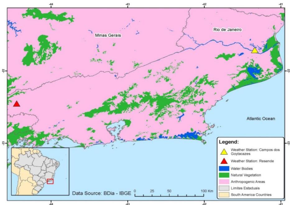 Figure 1: Study area comprising an expanded space in the Metropolitan Region of Rio de Janeiro. Water bodies in blue, natural vegetation in green, and areas with human action in pink. The stars signal the location of the INMET weather stations used in this study. ## III. RESULTS Based on the CALIOP sensor data series, the values of the monthly mean totals of the AOD at $532\mathrm{nm}$ for the RMRJ represented in Figure 2 were first calculated. It can be observed that the AOD has a well-defined seasonal behavior. The highest values were observed between August and November. The meteorological stations used as a source of rainfall data are in the central portion and on the periphery of the study area to represent the rainfall behavior throughout the region. These stations (indicated in Figure 1) were chosen for having the most comprehensive data series and for representing extreme regions within the study area. Considering the synoptic-scale movements, due to the size of the study area, the pluviometric data points have similar behavior. During this period, there is a transition between the driest months of winter and the beginning of the wettest period of spring [23]. In addition, a secondary peak is also observed in the elevation of optical thickness in May. This month presents a considerable drop in the rate of precipitation and cloudiness, which enables the highest accumulation of particles in the atmosphere. 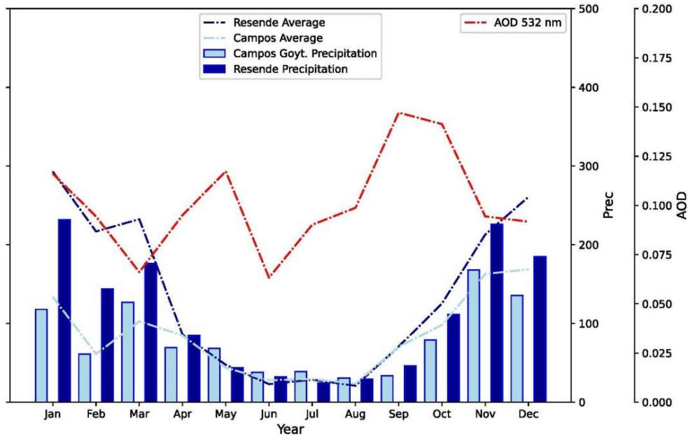 Figure 2: Average monthly totals of Aerosol Optical Depth from the CALIPSO satellite, with a study period from 2006 to 2019, are represented in red. Light (dark) blue bars indicate precipitation values from INMET's normals for the cities of Campos dos Goytacazes (Resende). The blue lines represent the average precipitation over the period between 2006 and 2019. To examine the year-round distribution of various atmospheric aerosol types, we conducted a classification using CALIPSO VFM. The results are shown in Table 2. Based on these results, Figure 3 was constructed, which shows the proportion of pixels classified as smoke, dust, and marine to the total number of verified pixels. The other types of aerosols (polluted continental, clean continental, and polluted dust) did not show significant levels and, therefore, were omitted in this figure. This figure was constructed to remove the seasonal effect of sea salt to analyze the proportions of smoke and dust in the total composition of atmospheric aerosols in the region. This is because marine aerosol, which is always present, exhibits a seasonal variation that strongly depends on the positioning of the South Atlantic Subtropical Anticyclone. In other words, the graphically represented values correspond to the total percentage that each type of aerosol (excluding marine aerosol) presents in the study area. The absolute values obtained and the standard error are shown in Table 2. These values indicate the total percentage of observation for each type of aerosol. The standard error was calculated as it represents a critical measure for understanding the variability and precision of statistical estimates. As can be observed in Table 2, the values obtained for the standard error are minimal, which indicates the more reliable the estimate. It is also verified that the pixels classified as dust are the most common after the marine, reaching values above the marine during Jan (39.7%), Feb (48.2%), Jul (44.4%), and Dec (54.1%). They represent all types of mineral particles originating from the erosion processes of rocks and soil, which are suspended in the atmosphere. Pixels classified as marine aerosols represent a large part of the classifications, exceeding 40 percent in 7 of the 12 months of the year. The reason may be due to the circulation of the South Atlantic Subtropical High (ASAS) [24] and the sea breeze [25] that causes the advection of this type of aerosol to the study area. As for the pixels classified as smoke type, the highlight goes to January (wet season) and August (dry season), where the proportion of this type reaches values of $34.7\%$ (being the most important). Table 2: The percentage contribution of each type of aerosol and the sample's standard error value. <table><tr><td>Month</td><td>Marine (%) – (Standard error)</td><td>Dust (%) – (Standard error)</td><td>Smoke(%) – (Standard error)</td></tr><tr><td>Jan</td><td>29.5 - (0.014)</td><td>39.7 – (0.048)</td><td>30.8 – (0.047)</td></tr><tr><td>Feb</td><td>29.7 - (0.019)</td><td>48.2 – (0.039)</td><td>22.1 – (0.047)</td></tr><tr><td>Mar</td><td>63.8 - (0.016)</td><td>30.7 – 0.054)</td><td>5.5 – (0.018)</td></tr><tr><td>Apr</td><td>47.6 - (0.020)</td><td>39.0 – (0.046)</td><td>13.4 – (0.041)</td></tr><tr><td>May</td><td>59.9 - (0.037)</td><td>31.0 – (0.055)</td><td>9.1 – (0.027)</td></tr><tr><td>Jun</td><td>64.6 - (0.041)</td><td>30.7 – (0.049)</td><td>4.7 – (0.022)</td></tr><tr><td>Jul</td><td>41.5 - (0.026)</td><td>44.4 – (0.058)</td><td>14.1 – (0.041)</td></tr><tr><td>Aug</td><td>30.7 - (0.029)</td><td>34.6 – (0.033)</td><td>34.7 – (0.064)</td></tr><tr><td>Sep</td><td>53.9 - (0.036)</td><td>36.6 – (0.047)</td><td>9.5 – (0.042)</td></tr><tr><td>Oct</td><td>47.1 - (0.027)</td><td>41.0 – (0.051)</td><td>11.9 – (0.025)</td></tr><tr><td>Nov</td><td>49.2 - (0.034)</td><td>42.4 – (0.049)</td><td>8.4 – (0.018)</td></tr><tr><td>Dec</td><td>29.3 - (0.017)</td><td>54.1 – (0.062)</td><td>16.6 – (0.030)</td></tr></table> 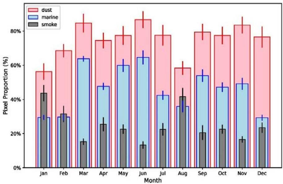 Figure 3: Total pixels classified as smoke (gray), marine (blue) and dust (red). The total is in percentage, in relation to the total value of pixels. The data refer to the CALIPSO satellite's Vertical Feature Mask product. Period 2006 to 2019. From the CALIOP sensor data, the trend in the proportion of these aerosols during the study period was also estimated. Figure 4 shows that the proportion of dust aerosols has been increasing significantly over this period compared to the presence of marine aerosols and smoke. These results align with the findings in [26], which demonstrated that this region has been experiencing increased aridity throughout nearly all months of the year, leading to a concurrent rise in diffuse solar radiation, particularly during the dry season. 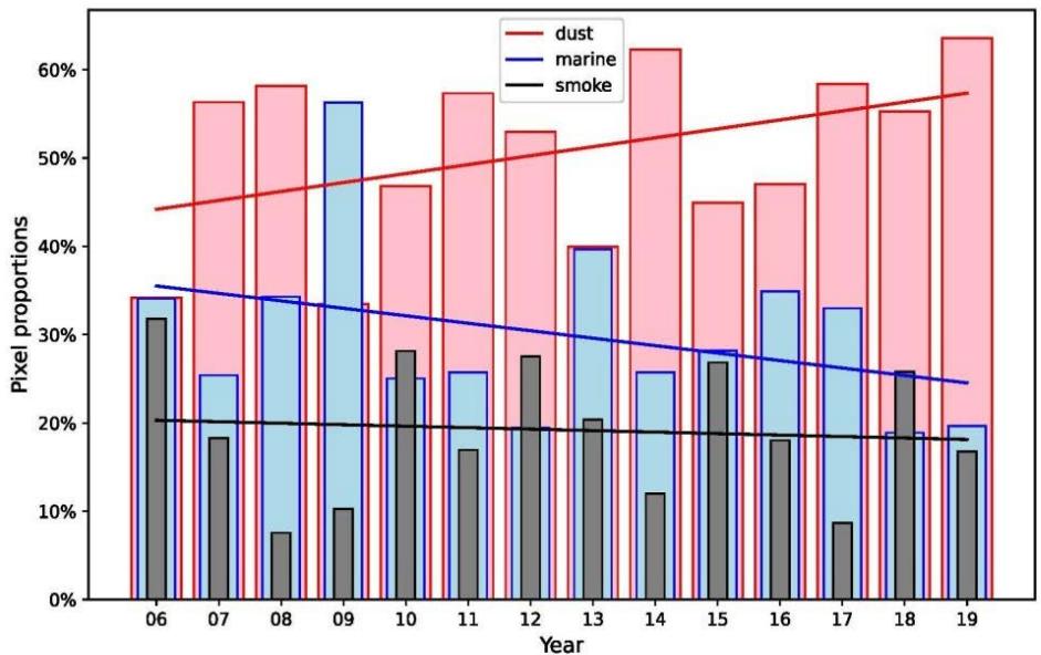 Figure 4: Trend of total pixels classified as smoke (gray), marine (blue) and dust (red). The total is in percentage, in relation to the total value of pixels. The data refer to the CALIPSO satellite's Vertical Feature Mask product. Period 2006 to 2019. It can be observed that the AOD has a well-defined seasonal behavior. The highest values were observed between August and November. The meteorological stations used as a source of rainfall data are in the central portion and on the periphery of the study area to represent the rainfall behavior throughout the region. Considering the large-scale movements, due to the size of the study area, the pluviometric data points have similar behavior. During this period, there is a transition between the driest months of winter and the beginning of the wettest period of spring [23]. In addition, a secondary peak is also observed in the elevation of optical thickness in May. This month presents a considerable drop in the rate of precipitation and cloudiness. To supplement the analysis conducted using CALIOP sensor data, an additional analysis was performed utilizing the data from the MERRA-2 reanalysis. 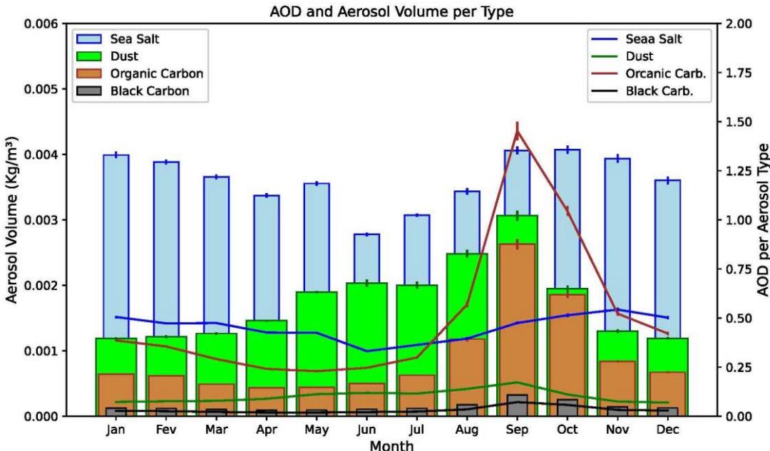In Figure 5, the totals of optical scattering and aerosol volume in the atmosphere can be observed. Notably, the volumes of black and organic carbon exhibit pronounced seasonality, with a substantial difference between the total observed during the dry season (May-September) and the total observed during the wet season (October-March). On the other hand, aerosols of mineral origin do not show significant variation throughout the year. Likewise, sea salt does not display a pronounced seasonal signal, showing peaks in the wet and dry months (summer and spring) and the dry months (autumn and winter). Despite not showing a pronounced seasonal signal, it is present throughout the year in a significant manner, as mapped in the literature. When examining scattering patterns, it's evident that carbonaceous aerosols exhibit distinct seasonality. In the case of mineral aerosols, their atmospheric volume magnitude doesn't result in significant changes in their optical characteristics. Moreover, the elevated values of pixels classified as black carbon in January can be attributed to their hydrophobic properties [4], as other aerosol types are typically employed as condensation nuclei. As shown in Figure 5, marine aerosols are the most prevalent in the study area, however, they do not have the most significant impact on the total absolute scattering. On the other hand, carbonaceous aerosols substantially contribute to the seasonal variation in total scattering, with their peak values coinciding with the peaks in the total optical depth variation for atmospheric aerosols. Their substantial variation is due to being more easily removed from the atmosphere by precipitation. Aerosols of mineral origin, in contrast, showed no significant seasonal variation. Another notable characteristic of atmospheric aerosols is that the volume of particulate matter in the atmosphere is not necessarily proportional to their effects on optical depth, as can be observed in Table 3. The table presents the coefficients of variation for the different quantities related to aerosols measured by MERRA-2.  Figure 5: Total volume (bars) and optical thickness (line) for aerosol types. In orange, data refers to organic carbon; in blue, those refer to sea salt; in green, those refer to dust; and in light black, those refer to black carbon. Data are from the MERRA2 reanalysis, with a study period from 2006 to 2019. Table 3: Annual Variation Coefficient of aerosols optical depths and volume. The data refer to the MERRA-2 aerosols products. Period 2006 to 2019. <table><tr><td colspan="2">Annual Variation Coefficient</td></tr><tr><td>Organic Carbon Optical Depth</td><td>3</td></tr><tr><td>Black Carbon Optical Depth</td><td>0.1</td></tr><tr><td>Sea Salt Optical Depth</td><td>0.1</td></tr><tr><td>Dust Optical Depth</td><td>0.1</td></tr><tr><td>Organic Carbon</td><td>4.5x10-4</td></tr><tr><td>Black Carbon</td><td>3.1x10-5</td></tr><tr><td>Sea Salt</td><td>4.2x10-5</td></tr><tr><td>Dust</td><td>1.8x10-4</td></tr></table> The seasonality of marine aerosols in the atmosphere is linked to the incursion of sea winds in the study area, as can be seen in Figure 6, which represents the hodography generated from METAR message data from Tom Jobim International Airport in the city of Rio de Janeiro. In the synoptic context, the position and intensity of the South Atlantic Subtropical Anticyclone (ASAS) system most interfere with the advection of maritime air. In winter, this system is positioned more to the southwest, making the atmosphere of the Southeast Region of Brazil more stable and the winds less intense. In summer, ASAS helps transport particles from the sea to the region [24, 27]. Thus, while the other types of aerosols decrease their concentrations in the atmosphere in the summer due to precipitation, the concentration of sea salt is maintained due to the advection of air coming from the ocean. On a smaller scale, there is a configuration of sea breezes throughout the year, contributing to the incursion of aerosols in the study area. 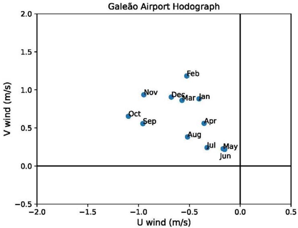 Figure 6: Hodograph of monthly average winds, from 1 to 12, obtained with observed data from METAR, located at Tom Jobim International Airport in Rio de Janeiro, for the sampling period from 2006 to 2019. To better understand the origin of the different types of aerosols, the HYSPLIT model was used, which made it possible to study the retro trajectories of air masses in the study area. Figure 7 represents the retrotrajectories of the air masses that ended in the study area. Each of the twelve images refers to the total number of simulations performed each month during the sixteen years of the study period. The retrojectives are grouped into clusters that were divided using the elbow method. There is no apparent connection between the direction and direction of the trajectories with the time of year. What can be seen in the simulations is that there is a trend of increasing advection of sea air in the summer months (DJF). This result was expected since, in the summer months, as previously mentioned, there is a more significant influence of the winds coming from the ASAS. As a result, the atmospheric circulation related to the anticyclone is northeast, mainly wind in the study area, which results in greater advection and, consequently, a greater concentration of sea salt (marine aerosols) during these months. Similarly, practically half of the simulations had continental coordinates as their starting point in June and July. This result is consistent, considering that the frequency of cold fronts increases in winter. Additionally, the westward shift of the ASAS center extends further into the continent during the summer months [24]. With this configuration of the ASAS, the incursion of the northeast winds in the study area decreases, as indicated in Figures 6 and 7. Consequently diminishing the trajectories that characterize air masses originating from the sea. Thus, there is evidence that the optical thickness peaks that occur in winter are linked to local sources of aerosols.            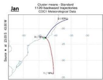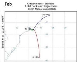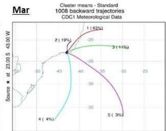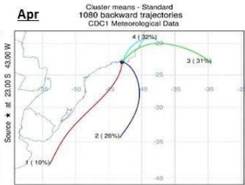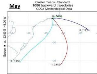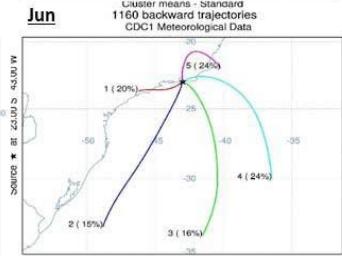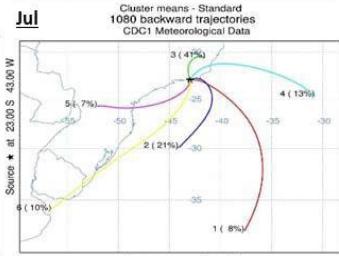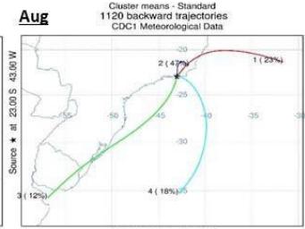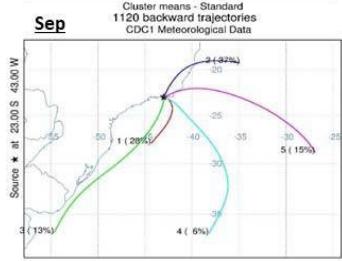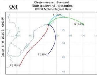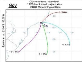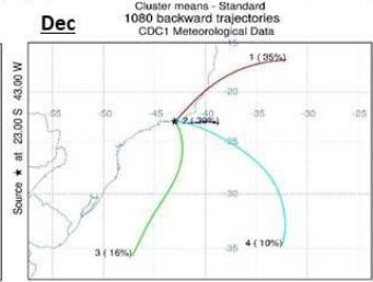 Figure 7: Retrotrajectories clusters of air masses, separated by month (compiled from 2006 to 2019). As the results showed that the greatest seasonal variations are related to carbonaceous aerosols, commonly produced by burning biomass and fossil combustion, an analysis was performed with data from the MCD64 product from MODIS [22] on the presence of fires near the study area. The standardized anomalies were calculated to generate a more complete analysis of the aerosols, which are shown in Figure 8. The graphs represent the temporal evolution of the standardized anomalies of the density of particulate matter in the atmosphere, separated monthly. Figure 8a shows the curves corresponding to the total thickness of the MERRA-2 reanalysis: Black Carbon, Sea Salt, AOD, and Dust. Figure 7b shows the totals of Black Carbon, AOD of CALIPSO, POLLCC (Polluted Continental) of CALIPSO, and Burnt Area of the product MCD64 of MODIS. Finally, in Figure 7c, the pixels classified by the Vertical Feature Mask are represented as POLLCC, DUST, and MARINE. This last graph also represents CALIPSO's AOD 532 and AOD 1064. To compare the behavior between the historical series of the data used, a correlation table was built in Table 4. In other words, the matrix supports the evaluation of how the reanalysis represents the atmospheric aerosols with reference to the data observed by the satellite. The Table 4 shows that the MERRA black carbon has a $94\%$ correlation with the MCD64 fire product and $93\%$ with the aerosols classified as smoke by the CALIPSO satellite. Furthermore, the correlation between CALIPSO smoke and MCD64 is $97\%$. Therefore, the representation of this type of aerosol seems to be in accordance with the reanalysis. When analyzing the sea salt, there is a negative correlation. In other words, there is no good representation of sea salt by the MERRA-2 reanalysis, considering the CALIPSO VFM data as a validator. The AOD 532 and 1064 correlation with the MERRA-2 AOT 550nm is 77 and $78\%$, respectively. The correlation value of this quantity is not so high because they are measurements at different wavelengths. The correlation between CALIPSO and MERRA-2 dust products is $78\%$. Therefore, there is evidence that fire products' representation is better than dust aerosols. It is also necessary to consider that the two products have different methods for classifying each aerosol type. Table 4: Correlation matrix of CALIPSO, Merra-2, and MODIS MCD64 products. Period 2006 to 2019. <table><tr><td></td><td>(1)</td><td>(2)</td><td>(3)</td><td>(4)</td><td>(5)</td><td>(6)</td><td>(7)</td><td>(8)</td><td>(9)</td><td>(10)</td></tr><tr><td colspan="11">MERRA-2</td></tr><tr><td>(1): Black Carbon</td><td>1.00</td><td>0.53</td><td>0.96</td><td>0.70</td><td>0.93</td><td>0.09</td><td>0.86</td><td>0.77</td><td>0.78</td><td>0.94</td></tr><tr><td>(2): Sea Salt</td><td>0.53</td><td>1.00</td><td>0.70</td><td>-0.110</td><td>0.45</td><td>-0.29</td><td>0.38</td><td>0.68</td><td>0.55</td><td>0.48</td></tr><tr><td>(3): AOT</td><td>0.96</td><td>0.70</td><td>1.00</td><td>0.50</td><td>0.86</td><td>-0.03</td><td>0.76</td><td>0.78</td><td>0.75</td><td>0.87</td></tr><tr><td>(4): Dust</td><td>0.70</td><td>-0.11</td><td>0.50</td><td>1.00</td><td>0.69</td><td>0.59</td><td>0.78</td><td>0.46</td><td>0.61</td><td>0.66</td></tr><tr><td colspan="11">CALIPSO</td></tr><tr><td>(5): Smoke</td><td>0.93</td><td>0.45</td><td>0.86</td><td>0.69</td><td>1.00</td><td>0.08</td><td>0.89</td><td>0.76</td><td>0.73</td><td>0.97</td></tr><tr><td>(6): Marine</td><td>0.09</td><td>-0.29</td><td>-0.03</td><td>0.59</td><td>0.08</td><td>1.00</td><td>0.39</td><td>0.13</td><td>0.41</td><td>-0.01</td></tr><tr><td>(7): Dust</td><td>0.86</td><td>0.38</td><td>0.76</td><td>0.78</td><td>0.89</td><td>0.39</td><td>1.00</td><td>0.76</td><td>0.86</td><td>0.82</td></tr><tr><td>(8): AOD 532</td><td>0.77</td><td>0.68</td><td>0.78</td><td>0.46</td><td>0.76</td><td>0.13</td><td>0.76</td><td>1.00</td><td>0.84</td><td>0.77</td></tr><tr><td>(9): AOD 1064</td><td>0.78</td><td>0.55</td><td>0.75</td><td>0.61</td><td>0.73</td><td>0.41</td><td>0.86</td><td>0.84</td><td>1.00</td><td>0.71</td></tr><tr><td colspan="11">MCD64</td></tr><tr><td>(10): B. Area</td><td>0.94</td><td>0.48</td><td>0.87</td><td>0.66</td><td>0.97</td><td>-0.01</td><td>0.82</td><td>0.77</td><td>0.71</td><td>1.00</td></tr></table> In Figure 8, a typical behavior can be observed in all graphs, which is most with higher anomalies between August and October. The highest values of black carbon, smoke, burned area, dust, and optical thickness are found in these months. The only curve that does not behave similarly to the others is that of sea salt, as shown by the two data sources. This type of aerosol has peaks in the dry season, and, in addition, it also has peaks when the center of the ASAS is further away from the continent. Considering the data from the MERRA-2 reanalysis, the dust and sea salt aerosols bear little resemblance to the variation patterns in aerosols' general scattering. While in CALIPSO, despite the correlation with marine aerosols remaining low, dust aerosols have a 76 percent correlation with optical thickness. The two data sources highly correlated with thickness and optical scattering for carbonaceous aerosols. In addition, the number of scars in the burned area also shows a high correlation with the carbonaceous aerosol samples and, consequently, with the mentioned optical properties. This indicates that, in fact, in the study region, the type of aerosol responsible for the main variations in the optical properties of the atmosphere is carbonaceous aerosols. This contribution occurs mainly through emissions from the fires located in the study region itself.  Figure 8: Monthly average standardized anomalies for the period 2006 to 2019, using MERRA-2 data (8a), the comparison between CALIPSO, MERRA, and MODIS data (8b) and CALIPSO data (8c). In Figures 8a and 8c, the colors of the lines represent purple, the aerosol optical thickness data; blue, marine aerosol data; red, dust data; and black, the smoke and/or black carbon data. In Figure 8b, the color black represents the black carbon data from MERRA-2 and the smoke data from the VFM from CALIPSO, the red color represents the burned area data from MCD64, and, in purple, the optical thickness data from the CALIPSO aerosols. ## IV. CONCLUSION This study aimed to conduct a temporal analysis of the primary aerosol characterization in a region centered on the Metropolitan Region of Rio de Janeiro, Brazil, examining their origin based on air mass back trajectories. The chosen study area is Brazil's second-largest conurbation and the country's second-most economically important region. Moreover, it is a region near the Atlantic coast with considerable ecological diversity. It has utilized remote sensing data from the CALIOP (Cloud-Aerosol Lidar with Orthogonal Polarization) sensor aboard the CALIPSO satellite. CALIOP stands out as one of the primary remote observation instruments for aerosol studies. In addition to this, it has incorporated data from the Modern-Era Retrospective Analysis Version 2 (MERRA-2) reanalysis to complement our analysis. MERRA-2 considers various physical processes involving aerosols. Simulations were conducted using the Hybrid Single Particle Lagrangian Integrated Trajectory (HYSPLIT) model for tracking air masses and gaining insight into their origins, which transport these particles. Furthermore, data from the Moderate Resolution Imaging Spectroradiometer (MODIS) sensor, with high-resolution products for fire studies, were integrated into the analysis. The study period, spanning from 2006 to 2019, was chosen primarily due to the availability of CALIOP sensor data, which commenced its operations in 2006 and extends until 2019, the year preceding the suspension of activities due to the COVID-19 pandemic. From a meteorological perspective, this period was marked by a drier spell compared to the climatology of the area located further northeast of the region (Campos dos Goytacazes station). In the western region (Resende station), the average precipitation closely adhered to the climatological precipitation pattern. It was observed that AOD has a well-defined seasonal behavior. The highest values were observed between August and November, with a peak of 0.15 in September, the transition period between the driest months of winter and the beginning of the wettest period of spring. A secondary peak was also observed, with a value of 0.10 in the optical thickness values in May, a month that presents a considerable drop in the average precipitation rate. The results show that the pixels classified as dust are the most common after the marine aerosols, reaching total values above the marine during Jan (39.7%), Feb (48.2%), Jul (44.4%), and Dec (54.1%) months. They represent all types of mineral particles originating from the erosion processes of rocks and soil, which are suspended in the atmosphere. Pixels classified as marine aerosols represent a large part of the classifications, exceeding 40 percent in 7 of the 12 months of the year, and smoke is more important during Aug (34.7%). The standard error for all data was calculated as it represents a critical measure for understanding the variability and precision of statistical estimates. The values obtained for the standard error are minimal, which indicates the more reliable the estimate. From the CALIOP sensor data, the trend in the proportion of these aerosols during the study period shows that the proportion of dust has increased significantly over this period compared to the presence of marine aerosols and smoke. These results align with other studies, which demonstrated that this region has been experiencing increased aridity throughout nearly all months of the year, leading to a concurrent rise in diffuse solar radiation, particularly during the dry season. What was also observed in this study were the highest AOD values during the dry season. It has shown that each type of aerosol contributes differently to the optical thickness of the atmosphere. Marine aerosols are the most present in the study area. However, they are not the ones that most impact the total amount and absolute seasonality of the total scattering. The variation throughout the year in the amount of marine aerosols is linked to the incursion of sea winds in the study area, particularly the position and intensity of the South Atlantic Subtropical High (ASAS). In addition, sea salt aerosols need a better atmospheric representation by the MERRA2 reanalysis compared to the data observed by the CALIPSO satellite. On the other hand, carbonaceous aerosols have the highest coefficients of variation among the optical thicknesses listed, even with lower absolute volumes. What it indicates that it is the type of particulate that most contributes to changes in optical characteristics in the study area during the year. Dust aerosols also show well-evidenced seasonality. In addition to the local source, they are brought by continental trajectories and are more present in winter, with the lowest precipitation rates. In this period, the Subtropical High of the South Atlantic is more evident. With a more significant continental portion, therefore, the winter values of this type of aerosol are higher. Contrasting this idea, the trajectories analyzed in the study period (2006-2019) indicate a more significant predominance in the northeast direction in the summer months. The study of retro trajectories made it possible to identify that the optical thickness peaks that occur in winter are linked to local sources of aerosols. As the results showed the carbonaceous aerosols presenting the most significant seasonal variations, it was possible to conclude through the analysis of data from burned areas (MD64 from MODIS), that the origin of these aerosols is linked to biomass burning and fossil combustion in the study region, as observed through the correlations between the black carbon series, MCD64, and optical thickness. Therefore, the type of aerosol that most impacts the seasonality of the optical properties of the atmosphere over the Rio de Janeiro Region is carbonaceous aerosols. Everything indicates that emissions are governed by the distribution of fires throughout the year in the study area and other biomes. In addition, sea salt aerosols are the most common in the region during most of the year. The use of CALIPSO satellite data provides a detailed analysis of aerosol presence in the atmosphere. Its classification is based on algorithms considering Particle Depolarization Ratio, Layer-Integrated Attenuated Backscatter, and Layer Top and Base Altitudes. This study used only aerosol types with the highest classification levels, including marine, dust, and smoke. Other aerosol types, such as polluted continental, clean continental, and polluted dust, did not exhibit significant levels and were therefore omitted. Remote sensing data allows for better spatial coverage. However, some local events may be missed due to its temporal coverage of one pass every 16 days. The results indicate that in the study area, despite being a coastal region with relatively dense vegetation, dust particles have been increasing over the past few years. This is likely due to reduced precipitation rates, which allow particles to linger in the atmosphere for extended periods, and wind erosion that injects soil particles from the surface into the atmosphere due to disorganized urban infrastructure. These totals and proportions are crucial for modeling the physical processes of the atmosphere and aerosol-cloud interaction. They play a significant role in understanding energy and the hydrological cycle in the Rio de Janeiro region, allowing for more realistic data in weather and climate modeling. Future work should include vertical profiles of aerosols and the use of data from new satellites such as the Sentinel series. ### Funding The authors declare that no funds, grants, or other support were received during the preparation of this manuscript. Author Contributions Filipe Pungirum and José Ricardo de Almeida Franca wrote and structured the entire article, generated the manuscript figures, and analyzed the results. Edson Pereira Marques Filho collaborated with exploring climate data and revised the paper. #### Data Availability The datasets generated during and/or analyzed during the current study are available from the organization that maintains the data on reasonable request. #### Conflicts of Interest The authors declare that they have no known competing financial interests or personal relationships that could have appeared to influence the work reported in this paper.

Generating HTML Viewer...

References

27 Cites in Article
Binita Pathak,Gayatry Kalita,K Bhuyan,P Bhuyan,K Moorthy (2010). Aerosol temporal characteristics and its impact on shortwave radiative forcing at a location in the northeast of India.
Dennis Lamb,Johannes Verlinde (2011). Physics and Chemistry of Clouds.
V Ramanathan,P Crutzen,J Kiehl,D Rosenfeld (2016). Unknown Title.
G Mcmeeking,N Good,M Petters,G Mcfiggans,H Coe (2011). Influences on the fraction of hydrophobic and hydrophilic black carbon in the atmosphere.
Zhuzi Zhao,Junji Cao,Zhenxing Shen,Baiqing Xu,Chongshu Zhu,L Chen,Xiaoli Su,Suixin Liu,Yongming Han,Gehui Wang,Kinfai Ho (2013). Aerosol particles at a high‐altitude site on the Southeast Tibetan Plateau, China: Implications for pollution transport from South Asia.
C Hoose,O Möhler (2012). Heterogeneous ice nucleation on atmospheric aerosols: a review of results from laboratory experiments.
A Khain,B Lynn,J Dudhia (2010). Aerosol Effects on Intensity of Landfalling Hurricanes as Seen from Simulations with the WRF Model with Spectral Bin Microphysics.
Sushant Das,Sagnik Dey,S Dash,G Giuliani,F Solmon (2015). Dust aerosol feedback on the Indian summer monsoon: Sensitivity to absorption property.
E N'datchoh,I Diallo,A Konaré,S Silué,K Ogunjobi,A Diedhiou,M Doumbia (2018). Dust induced changes on the West African summer monsoon features.
Hannele Korhonen,Kenneth Carslaw,Piers Forster,Santtu Mikkonen,Neil Gordon,Harri Kokkola (2010). Aerosol climate feedback due to decadal increases in Southern Hemisphere wind speeds.
D Winker,M Vaughan,A Omar,Y Hu,K Powell,Z Liu,W Hunt,S Young (2009). Overview of the CALIPSO Mission and CALIOP Data Processing Algorithms.
Pengfei Tian,Xianjie Cao,Lei Zhang,Naixiu Sun,Lu Sun,Timothy Logan,Jinsen Shi,Yuan Wang,Yuemeng Ji,Yun Lin,Zhongwei Huang,Tian Zhou,Yingying Shi,Renyi Zhang (2017). Aerosol vertical distribution and optical properties over China from long-term satellite and ground-based remote sensing.
Man-Hae Kim,Ali Omar,Jason Tackett,Mark Vaughan,David Winker,Charles Trepte,Yongxiang Hu,Zhaoyan Liu,Lamont Poole,Michael Pitts,Jayanta Kar,Brian Magill (2018). The CALIPSO Version 4 Automated Aerosol Classification and Lidar Ratio Selection Algorithm.
M Rienecker,M Suarez,R Gelaro,R Todling,J Bacmeister,E Liu,M Bosilovich,S Schubert,L Takacs,G Kim,S Bloom,J Chen,D Collins,A Conaty,A Da Silva,W Gu,J Joiner,R Koster,R Lucchesi,A Molod,T Owens,S Pawson,P Pegion,C Redder,R Reichle,F Robertson,A Ruddick,M Sienkiewicz,J Woollen (2011). MERRA: NASA's modern-era retrospective analysis for research and applications.
A Stein,R Draxler,G Rolph,B Stunder,M Cohen,F Ngan (2015). Noaa's hysplit atmospheric transport and dispersion modeling system.
Norikazu Kinoshita,Keisuke Sueki,Kimikazu Sasa,Jun-Ichi Kitagawa,Satoshi Ikarashi,Tomohiro Nishimura,Ying-Shee Wong,Yukihiko Satou,Koji Handa,Tsutomu Takahashi,Masanori Sato,Takeyasu Yamagata (2011). Assessment of individual radionuclide distributions from the Fukushima nuclear accident covering central-east Japan.
Glenn Rolph,Roland Draxler,Ariel Stein,Albion Taylor,Mark Ruminski,Shobha Kondragunta,Jian Zeng,Ho-Chun Huang,Geoffrey Manikin,Jeffery Mcqueen,Paula Davidson (2009). Description and Verification of the NOAA Smoke Forecasting System: The 2007 Fire Season.
Christos Efstathiou,Sastry Isukapalli,Panos Georgopoulos (2011). A mechanistic modeling system for estimating large-scale emissions and transport of pollen and co-allergens.
B Stunder,J Heffter,R Draxler (2007). Airborne Volcanic Ash Fore-cast Area Reliability.
Hongbin Yu,Mian Chin,Tianle Yuan,Huisheng Bian,Lorraine Remer,Joseph Prospero,Ali Omar,David Winker,Yuekui Yang,Yan Zhang,Zhibo Zhang,Chun Zhao (2015). The fertilizing role of African dust in the Amazon rainforest: A first multiyear assessment based on data from Cloud‐Aerosol Lidar and Infrared Pathfinder Satellite Observations.
M Kanamitsu,W Ebisuzaki,J Woollen,S.-K Yang,J Hnilo,M Fiorino,G Potter (2002). NCEP-DOE AMIP-II Reanalysis (R-2).
L Giglio,G Van Der Werf,J Randerson,G Collatz,P Kasibhatla (2006). Global estimation of burned area using MODIS active fire observations.
M Pristo,C Dereczynski,P De Souza,W Menezes (2018). Climatologia de Chuvas Intensas no Município do Rio de Janeiro.
C Bastos,N Ferreira (2008). Análise Climatológica da Alta Subtropical do Atlântico Sul.
Luiz Pimentel,Edilson Marton,Mauricio Silva,Pedro Jourdan (2014). Caracterização do regime de vento em superfície na Região Metropolitana do Rio de Janeiro.
Edson Marques Filho,Amauri Oliveira,Willian Vita,Francisco Mesquita,Georgia Codato,João Escobedo,Mariana Cassol,José França (2016). Global, diffuse and direct solar radiation at the surface in the city of Rio de Janeiro: Observational characterization and empirical modeling.
Claudine Dereczynski,Juliana Oliveira,Christiane Machado (2009). Climatologia da precipitação no município do Rio de Janeiro.
No ethics committee approval was required for this article type.
Data Availability
Not applicable for this article.
How to Cite This Article
Filipe Pungirum. 2026. \u201cAerosol Typology and Trajectories in the Metropolitan Region of Rio de Janeiro, Brazil\u201d. Global Journal of Human-Social Science - B: Geography, Environmental Science & Disaster Management GJHSS-B Volume 23 (GJHSS Volume 23 Issue B5).
Explore published articles in an immersive Augmented Reality environment. Our platform converts research papers into interactive 3D books, allowing readers to view and interact with content using AR and VR compatible devices.
Your published article is automatically converted into a realistic 3D book. Flip through pages and read research papers in a more engaging and interactive format.
Our website is actively being updated, and changes may occur frequently. Please clear your browser cache if needed. For feedback or error reporting, please email [email protected]
Thank you for connecting with us. We will respond to you shortly.