## I. INTRODUCTION In the fast-paced world of software engineering, accurate estimation of lead time is a critical factor that can significantly impact project planning, resource allocation, and overall project success. Lead time refers to the time taken from the inception of a software development task to its completion, encompassing various stages such as design, coding, testing, and deployment. Traditional methods of lead time estimation often suffer from subjectivity, imprecision, and a lack of adaptability to changing project dynamics. However, the rise of data-driven approaches and machine learning techniques has opened new possibilities for automating and improving lead time estimation. The dynamic field of software engineering encompasses the methodical design, development, testing, and maintenance of software systems. It involves using a methodical approach to software development, which includes defining requirements, coming up with solutions, writing code, and subjecting the finished result to rigorous testing. Together, software developers use a range of methodologies, including as Agile and DevOps, to continuously build and enhance software while reacting to shifting input and requirements. The methodology includes selecting appropriate programming languages and design patterns as well as managing version control, assuring security, and maintaining documentation. A combination of technical know-how, teamwork, project management, and a commitment to ethical considerations are required to produce reliable and efficient software solutions that address real-world problems the software industry The K-Means clustering algorithm is one such powerful technique that is gaining prominence in the software engineering domain. K-Means is an unsupervised machine learning approach that uses similarity to divide data into separate clusters. Its capacity to detect hidden patterns and structures in datasets makes it a great candidate for lead time estimating automation. K-Means can accurately forecast lead times for new activities by exploiting prior project data to find intrinsic correlations between development tasks and their related lead times. This paper presents an in-depth exploration of the K-Means clustering algorithm and its application to automate lead time estimation in software engineering projects. We will delve into the underlying principles of K-Means, its strengths, limitations, and how it can be fine-tuned to suit the unique characteristics of software development processes. Furthermore, we will discuss the challenges associated with implementing K-Means for lead time estimation and propose strategies to overcome them. The objective of this research is to equip software development teams, project managers, and stakeholders with a data-driven, efficient, and reliable lead time estimation tool that can facilitate better decision-making, resource allocation, and project planning. By harnessing the power of K-Means clustering, we aim to enhance the accuracy and efficiency of lead time estimation, ultimately leading to improved project management and successful software development endeavours. Software lead time estimation, a critical aspect of project management, employs various techniques to predict the time needed for software development projects. Among these techniques, analogy-based methods, neural networks, and Particle Swarm Optimization (PSO) play distinctive roles. Analogy-based methods leverage historical data from similar projects to estimate lead times. By comparing known project outcomes and characteristics to those of the current project, these methods extrapolate estimates. While intuitive and easily accessible, their accuracy relies heavily on the quality and relevance of historical data. Neural networks, a machine learning approach, demonstrate their strength in lead time estimation by learning complex patterns from historical data. These interconnected layers of nodes process input parameters to generate accurate predictions. Their ability to capture nonlinear relationships and adapt to diverse project variables makes them robust tools, particularly when adequate data is available for training. Particle Swarm Optimization, inspired by the social behaviour of birds flocking or fish schooling, employs optimization to estimate lead times. It simulates a population of particles traversing a solution space to find optimal estimates. Through iterative refinement, PSO converges towards accurate predictions by adjusting particle positions based on local and global information. ## II. RELATED WORKS In 2008, Kim[^1] et al. published the first study on JIT-SDP, where they described a set of input features for JIT-SDP models. Other research looked into input features that could be useful for JIT-SDP, like the day of the week or the time of day a software change was produced, and input features to make it possible to identify software changes that are difficult to fix. According to Shihab[^2]et al., the amount of lines of code contributed, the proportion of bug fixes to total file changes, the number of bug reports associated with a commit, and the developer experience are all reliable indications of software modifications that cause defects. Kamei[^3] et al. carried out a substantial empirical investigation to look into a variety of factors extracted from commits and bug reports as input features for JIT-SDP models. They considered 14 features grouped into five dimensions of diffusion, size, purpose, history and experience, and showed such features to be good indicators of defect-inducing software changes for yielding high predictive performance on both open source and commercial projects. Many subsequent studies have adopted these features. In 2022, Elvan Kula[^4]; Eric Greuter[^5]; Arie van Deursen[^6]; Georgios Gousios[^7] wrote late delivery of software projects and cost overruns have been common problems in the software industry for decades. Both problems are manifestations of deficiencies in effort estimation during project planning. With software projects being complex socio-technical systems, a large pool of factors can affect effort estimation and on-time delivery. To identify the most relevant factors and their interactions affecting schedule deviations in large-scale agile software development, we conducted a mixed-methods case study at ING: two rounds of surveys revealed a multitude of organizational, people, process, project and technical factors which were then quantified and statistically modelled using software repository data from 185 teams. We find that factors such as requirements refinement, task dependencies, organizational alignment and organizational politics are perceived to have the greatest impact on on-time delivery, whereas proxy measures such as project size, number of dependencies, historical delivery performance and team familiarity can help explain a large degree of schedule deviations. We also discover hierarchical interactions among factors: organizational factors are perceived to interact with people factors, which in turn impact technical factors. We compose our findings in the form of a conceptual framework representing influential factors and their relationships to on-time delivery. Our results can help practitioners identify and manage delay risks in agile settings, can inform the design of automated tools to predict schedule overruns and can contribute towards the development of a relational theory of software project management. In 2021, Lei Zou $^{8}$, Zidong Wang $^{9}$, Qing-Long Han $^{10}$, Donghua Zhou $^{11}$ wrote the full information estimation (FIE) problem is addressed for discrete time-varying systems (TVSs) subject to the effects of a Round-Robin (RR) protocol. A shared communication network is adopted for data transmissions between sensor nodes and the state estimator. In order to avoid data collisions in signal transmission, only one sensor node could have access to the network and communicate with the state estimator per time instant. The so-called RR protocol, which is also known as the token ring protocol, is employed to orchestrate the access sequence of sensor nodes, under which the chosen sensor node communicating with the state estimator could be modelled by a periodic function. A novel recursive FIE scheme is developed by defining a modified cost function and using a so-called "backward-propagation-constraints." The modified cost function represents a special global estimation performance. The solution of the proposed FIE scheme is achieved by solving a minimization problem. Then, the recursive manner of such a solution is studied for the purpose of online applications. For the purpose of ensuring the estimation performance, sufficient conditions are obtained to derive the upper bound of the norm of the state estimation error (SEE). Finally, two illustrative examples are proposed to demonstrate the effectiveness of the developed estimation algorithm. ## III. PROPOSED METHODOLOGY ### a) Particle Swarm Optimization (PSO) PSO was developed by Eberhart[^4] and Kennedy[^5] in 1995. It is swarm intelligence meta-Heuristic inspired by the group behaviour of birds flocks or fish schools. It is simple, fast and easy to understand. Similarly, to Genetic Algorithm (GAs), it is a population-based method, that is, it represents the state of the algorithm by a population, which is iteratively modified until a termination criterion is satisfied. In PSO, the potential solution called particle which searches the whole space by previous best position (pbest) and best position of the swarm (gbest). The fitness function can be evaluated by the following equation. $$ f _ {n} = \sum_ {j = 1} ^ {k} \sum_ {i = 1} ^ {n} | | x _ {i} ^ {j} - c _ {j} | | ^ {2} \tag {1} $$ Initially, position and velocity of the particles are expressed as follows $$ X _ {i} = \mathrm{L B} + \text{r and (U B - L B)} \tag{2} $$ $$ V _ {i} = \frac{L B + r and (U B - L B)}{\Delta t} \tag{3} $$ The velocity and positions values are updated during each iteration. Velocity update equation is given below $$ V_{i+1} = w V_i + c_1 \operatorname{rand} \frac{pbest_i - X_i}{\Delta t} + c_2 \operatorname{rand} \frac{pbest_i - X_i}{\Delta t} $$ Where, Xi is current position, Vi+1 is the velocity of next iteration, Vi is current velocity, Δt is the time interval, rand is a uniformly distributed random variable that can take any value between 0 and 1. Pbesti is the location of the particle that experiences the best fitness, gbesti is the location of the particle that experiences a global best fitness value, c1 and c2 are two positive acceleration constants responsible for degree of information, w represents inertia weight which is usually linearly decreasing during the iterations. Updating position is the last step in each iteration, it is updated using velocity vector. Position update equation is given below $$ X _ {i + 1} = X _ {i} + V _ {i + 1} \Delta t \tag {5} $$ Where, $X_{i+1}$ is the next position, $X_i$ is the current position, $V_{i+1}$ is the next velocity, $\Delta t$ is the time interval. Update the best fitness values at each generation, based on below equation $$ P _ {i} (t + 1) = \left\{ \begin{array}{c} P _ {i} (t) \\ X _ {i} (t + 1) \end{array} \right. f (X _ {i} (t + 1)) \leq f (X _ {i} (t)) $$ $$ f \left(X _ {i} (t + 1)\right) > f \left(X _ {i} (t)\right) \tag {6} $$ Where, $f$ denotes the fitness function Eq. (1), $Pi(t)$ stands for best fitness value and the coordination where the values are computed, $\mathrm{Xi(t)}$ is the current position, $t$ denotes the generation step. Update the velocity, position and fitness computations are repeated until the termination criteria is met. ### b) K-Means Clustering Algorithm(KMC) This K-means clustering is the best unsupervised learning algorithm. Using a certain number of clusters, it is simple and easy to classify a given data set. Initially, select the k centroids, then calculate the distance between each cluster centre and each object. Repeat the steps until no more changes are done. The objective function of k-means clustering is given as $$ f_{n} = \sum_{j=1}^{k} \sum_{i=1}^{n} \| \mathbf{x}_{i}^{j} - \mathbf{c}_{j} \|^{2} \tag{7} $$ Where, n is the number of data points, k is the number of clusters, \|\mathbf{x}_{i}^{j} - \mathbf{c}_{j}\|^{2} is the distance between each cluster centre and each object. The steps of k-means clustering is shown below 1. Place K points into the space which denotes initial group centroids. 2. The group closer to the centroid is assigned with a cluster. 3. When all the objects are assigned to the groups, the positions of K centroids are reallocated. 4. Repeat Steps 2 and 3 until the centroids no longer move. In this paper, combination of PSO and k-means clustering is used. PSO works efficiently for global search but its local search ability is poor. K-means clustering which produces local optimal solution due to initial partition but it does not work well for global search ability. Hence the proposed method overcome the limitation of K-means clustering, PSO offers global search methodology. Initially PSO is performed to find the location of cluster centroids. These locations of cluster centroids are given as input for the k-means clustering and provide optimal clustering solution. The steps for the proposed method is given below Step 1: Randomly generate particles and particles are grouped which creates population. Step 2: Position and velocity of particles are initialized using Equation (2) and (3). Step 3: Compute the fitness value using Eq. (6) Step 4: Position, velocity, gbest and pbest values of the particles are updated using Equation (4) and (5). Step 5: Repeat step (3) and (4) until one of the following termination conditions is satisfied. 5(a). The maximum number of iterations is exceeded. 5(b). The average change in centroid vectors is less than a predefined value.  Step 6: Input the number of clusters which is to be generated. Step 7: Compute the cluster centroids using the best positions of $k$ of PSO. Step 8: Compute the distance between the particles and centroids. Step 9: Cluster centroids of k-means clustering can be recomputed using Eq. (7). Step 10: Repeat the steps (8) and (9) until the centroids no longer move. 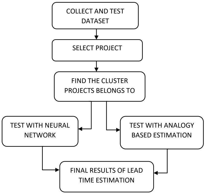The combination of PSO and k-means provides better clustering result compared to result of each individual technique. PSO is used to find the optimal solution, the output of PSO is given as input to the k-means to obtain the clustering result. Check if the number of projects in clusters is greater than or equal to 15. For analogy method the number of projects present in a cluster should be less than fifteen. There are two reasons for choosing based on 15 projects. First, each project in the dataset usually has at least 10 features to train the neural network properly. Second, when using combination of PSO and K-means clustering the minimum requirement is 15. Anything less than 15 will become useless for training Neural Network. Testing stage consists of following steps. The Euclidean distance between a particular project and cluster centre is measured. The it is done for all the projects, the one with minimum is chosen. If it is marked in the training stage as ABE, then ABE is used to estimate the lead time. Otherwise NN is applied to predict the lead time. Repeat the steps until all test projects are applied to the hybrid model. For each test project the MRE is calculated and the final result is computed based on MMRE and PRED. ## IV. ANALOGY BASED METHOD The most common example of analogy-based project estimation is case-based reasoning, where identical projects from the lesson learned are identified and used for estimation. They can be used in combination with collective expert opinion and formal models, Software lead time estimation by using an analogy-based tech commonly involves the following steps. 1. Measuring the values of identified metrics of the software project for which estimation is being performed (target project). 2. Finding a similar project from the repository. 3. Using the estimated effort values of the selected projects to use as an initial estimate for the target project. 4. Comparison of metric's value for the target project and selected project. 5. Adjustment of lead time estimates in view of the comparison performed in the previous step. ## V. NEURAL NETWORK Neural networks are a type of machine learning model inspired by the structure and function of the human brain. They are mathematical models composed of interconnected nodes, or neurons, that process information through a series of weighted connections. These connections allow neural networks to learn patterns and make predictions based on the input data. The artificial neural network is a powerful tool in the field of machine learning, as it can adapt and learn from data in a way that resembles human brain processing (Singh & Shrimali, 2019). It is important to understand the structure and functionality of neural networks in order to effectively utilize them for various applications in machine learning. Additionally, neural networks have layers, including an input layer, hidden layer(s), and an output layer. These layers help to organize and process the data, allowing for more accurate predictions or estimations. Furthermore, neural networks have been successfully applied in various fields including image recognition, natural language processing, and financial forecasting. By understanding the structure and functionality of neural networks, researchers and practitioners can effectively utilize these powerful machine learning models for various applications. In today's rapidly changing world, the significance of accurate weather forecasts cannot be overstated. In the context of neural networks, understanding their structure and functionality is crucial for effectively utilizing them in machine learning applications. Additionally, the widespread applications of neural networks in the control field, such as system identification and controller design, highlight their versatility and potential for solving complex problems. Overall, understanding the structure and functionality of neural networks is essential for harnessing their potential in machine learning applications and solving a variety of complex problems. In today's rapidly changing world, the significance of accurate weather forecasts cannot be overstated. Neural networks, with their ability to learn from data and make predictions, have wide-ranging applications in machine learning. ## VI. EXPERIMENTAL DESIGN ### a) Evaluation Criteria The research community realizes that MMRE, Pred(x) can be influenced by the presence of outliers, therefore, we used the following performance metrics to assess and compare the accuracy. ### b) Magnitude of Relative Error The error ratio between actual and predicted effort for each project instance in the dataset is computed using MRE. To calculate the fitness function, first the MRE is calculated for every project i. $$ MRE = \left| \frac{\text{Actual effort} - \text{Estimated Effort}}{\text{Actual Effort}} \right| \tag{8} $$ ### c) Mean Magnitude of Relative Error MMRE measure is used for assessing software estimation technique performance. The values of MRE is calculated for each software project instance. MMRE computes the average over $N$ number of project instances in the data-set. $$ M M R E = \frac {1}{N} \sum_ {i = 1} ^ {N} M R E \tag {9} $$ ### d) Percentage of Prediction PRED(x) represents the percentage of MRE that is less than or equal to the value x/100 among all projects. $$ \operatorname{PRED}(X) = \frac{100}{N} \left\{ \begin{array}{l l} 1 & \text{if MRE} \leq \frac{X}{100} \\ 0 & \text{otherwise} \end{array} \right. \tag{10} $$ where A is the number of projects with MRE less than or equal to X. N is the number of projects in test set. Usually the ideal value of X is $25\%$ in software development effort estimation and compared with various methods. Table No. 1: Time Estimation Table <table><tr><td>Algorithm</td><td>Time Estimation</td></tr><tr><td>Neural Network</td><td>3.73</td></tr><tr><td>ABE algorithm</td><td>0.78</td></tr></table> Table No. 2: Accuracy Table <table><tr><td>Algorithm</td><td>Accuracy</td></tr><tr><td>Neural Network</td><td>95.79</td></tr><tr><td>ABE algorithm</td><td>97.68</td></tr></table> Table No. 3: Loss comparison Table <table><tr><td>Algorithm</td><td>Loss</td></tr><tr><td>Neural Network</td><td>4.21</td></tr><tr><td>ABE algorithm</td><td>2.32</td></tr></table> ### e) Lead Time Estimation Lead time estimation is the process of predicting the amount of time it will take to complete a specific task, project, or deliver a product or service. It is a critical aspect of project management and supply chain management and is used in various industries, including manufacturing, logistics, and software development. Accurate lead time estimation helps organizations plan and allocate resources effectively, manage customer expectations, and avoid delays and disruptions in their operations. ### f) Leave-One-Out In this method a project is selected from the dataset as the target project. The ABE method is applied to estimate the effort of the target project by using all the remaining projects in dataset. Then the target project combined with the dataset and another project is selected as a target project. This procedure repeated until all the projects in dataset are estimated. Finally, the MRE and MMRE values are computed for each project ### g) Dataset Description Software to detect network intrusions protects a computer network from unauthorized users, including perhaps insiders. The intrusion detector learning task is to build a predictive model (i.e. a classifier) capable of distinguishing between "bad" connections, called intrusions or attacks, and "good" normal connections. The 1998 DARPA Intrusion Detection Evaluation Program was prepared and managed by MIT Lincoln Labs. The objective was to survey and evaluate research in intrusion detection. A standard set of data to be audited, which includes a wide variety of intrusions simulated in a military network environment, was provided. The 1999 KDD intrusion detection contest uses a version of this dataset. Lincoln Labs set up an environment to acquire nine weeks of raw TCP dump data for a local-area network (LAN) simulating a typical U.S. Air Force LAN. They operated the LAN as if it were a true Air Force environment, but peppered it with multiple attacks. The raw training data was about four gigabytes of compressed binary TCP dump data from seven weeks of network traffic. This was processed into about five million connection records. Similarly, the two weeks of test data yielded around two million connection records. A connection is a sequence of TCP packets starting and ending at some well- defined times, between which data flows to and from a source IP address to a target IP address under some well-defined protocol. Each connection is labelled as either normal, or as an attack, with exactly one specific attack type. Each connection record consists of about 100 bytes. Attacks fall into four main categories: - DOS: denial-of-service, e.g. sync flood; - R2L: unauthorized access from a remote machine, e.g. guessing password; - U2R: unauthorized access to local super user (root) privileges, e.g., various "buffer overflow" attacks; - Probing: surveillance and other probing, e.g., port scanning. It is important to note that the test data is not from the same probability distribution as the training data, and it includes specific attack types not in the training data. This makes the task more realistic. Some intrusion experts believe that most novel attacks are variants of known attacks and the "signature" of known attacks can be sufficient to catch novel variants. The datasets contain a total of 24 training attack types, with an additional 14 types in the test data only. ### h) Numerical Results In this paper, for training stage two clusters are considered. When Applying the PSO and k-means clustering to the intrusion detector learning dataset, the best situation is with two clusters. When it is more than two some clusters with one or two projects appeared not perfect for estimation. On the other hand, splitting projects in clusters size less than two decreases the performance of NN training. 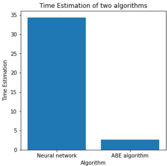 Fig. 1: Time Estimation of NN and ABE algorithm Results on all Data. Initially, the selected features from PSO is 19 are grouped into five clusters by k-Means clustering algorithm. Based on the number of projects in a cluster either ABE or NN is identified displayed the clusters formed from PSO and K-Means clustering algorithm. The identified method for cluster. Identifying a cluster for a project is done according to the maximum degree of membership function. First clusters are NN and second cluster are marked as ABE. 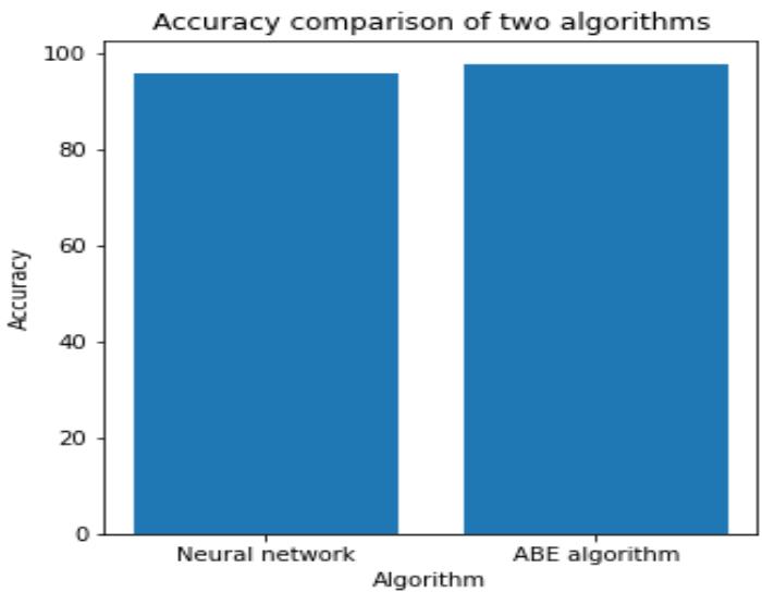 Fig. 2: Accuracy comparison of NN and ABE algorithm ## VII. RESULT Finally, from the Fig-1 and Fig-2, by comparing the Neural Network and Analogy Based Estimation, the accuracy of NN: $95.79\%$ and time taken for Neural Network: 34.34 seconds. Accuracy of ABE: $97.68\%$ and time taken by Analogue Based Estimation: 2.66921 seconds. The performance of ABE is better than NN, with less time taken and improved accuracy. ## VIII. CONCLUSION This paper proposes a hybrid scheme for clustering based on PSO and K-means algorithm. K-means algorithm paves way to predetermine the number of clusters by the end users which results in an improper clustering. Hence PSO algorithm is integrated with K-means algorithm to improve the better clustering result. This result is more efficient when applied to neural networks and ABE. ## IX. FUTURE WORK To perform the model compiling for the minimum accuracy. Time taken to done for the preprocessing the dataset is very low, when compared with the other techniques. Our future work is to implement other techniques for effort estimation for this method.

Generating HTML Viewer...

References

27 Cites in Article
A Sinha,P Malo,K Deb (2018). A review on bilevel optimization: From classical to evolutionary approaches and applications.
Ahmad Setiadi,Wahyutama Hidayat,Ahmad Sinnun,Ade Setiawan,Muhammad Faisal,Doni Alamsyah (2021). Analyze the Datasets of Software Effort Estimation With Particle Swarm Optimization.
Alvin Jian,Jia Tan,; Chun,Yong Chong,Aldeida Aleti (2023). Closing the Loop for Software Remodularisation -REARRANGE: An Effort Estimation Approach for Software Clustering-based Remodularisation.
Benoît Colson,Patrice Marcotte,Gilles Savard (2007). An overview of bilevel optimization.
D Vesset,C Gopal,C Olofson,D Schubmehl,S Bond,M Fleming (2018). Building an Understanding of Big Data Analytics.
D Aussel,C Lalitha (2018). Generalized Nash equilibrium problems.
Elvan Kula,Eric Greuter,Arie Van Deursen,Georgios Gousios (2021). Factors Affecting On-Time Delivery in Large-Scale Agile Software Development.
F Vandenbergh,A Engelbrecht (2006). A study of particle swarm optimization particle trajectories.
Guang-Min Wang,Xian-Jia Wang,Zhong-Ping Wan,Shi-Hui Jia (2007). An adaptive genetic algorithm for solving bilevel linear programming problem.
H Liu,L Gao,Q Pan (2011). A hybrid particle swarm optimization with estimation of distribution algorithm for solving permutation flowshop scheduling problem.
Ho Nhung,Vo Van Hai,Radek Silhavy,Zdenka Prokopova,Petr Silhavy (2022). Parametric Software Effort Estimation Based on Optimizing Correction Factors and Multiple Linear Regression.
H Mühlenbein,G Paaß (1996). From recombination of genes to the estimation of distributions I. Binary parameters.
J Agor,O Özaltın (2019). Feature selection for classification models via bilevel optimization.
Jiahai Wang (2007). A Novel Discrete Particle Swarm Optimization Based on Estimation of Distribution.
Z Koszty´ An,R Jakab,G Nov´ Ak,Hegedus Survive IT! survival analysis of IT project planning approaches.
Mona Najafi Sarpiri,; Mohammadreza,Soltan Aghaei,; Taghi,Javdani Gandomani (2021). Towards Better Software Development Effort Estimation with Analogy-based Approach and Nature-based Algorithms.
M Iqbal,M Montes De Oca (2006). An estimation of distribution particle swarm optimization algorithm.
Passakorn Phannachitta (2020). On an optimal analogy-based software effort estimation.
Pierre-Louis Poirion,Sonia Toubaline,Claudia D’ambrosio,Leo Liberti (2020). Algorithms and applications for a class of bilevel MILPs.
R Kulkarni,G Venayagamoorthy (2007). An Estimation of Distribution Improved Particle Swarm Optimization Algorithm.
Tao Zhang,Xiaofei Li (2018). The Backpropagation Artificial Neural Network Based on Elite Particle Swam Optimization Algorithm for Stochastic Linear Bilevel Programming Problem.
Javdani Taghi,Maedeh Gandomani,; Dashti,Zaiei Mina,Nafchi (2022). Hybrid Genetic-Environmental Adaptation Algorithm to Improve Parameters of COCOMO for Software Cost Estimation.
Usama Farooq,Mansoor Ahmed,Shahid Hussain,Faraz Hussain,Alia Naseem,Khurram Aslam (2022). Blockchain-Based Software Process Improvement (BBSPI): An Approach for SMEs to Perform Process Improvement.
Vo Hai,Ho Nhung,Zdenka Prokopova,Radek Silhavy,Petr Silhavy (2022). A New Approach to Calibrating Functional Complexity Weight in Software Development Effort Estimation.
Xiaotie Deng (1998). Complexity Issues in Bilevel Linear Programming.
Y Jiang,X Li,C Huang,X Wu (2013). Application of particle swarm optimization based on CHKS smoothing function for solving nonlinear bilevel programming problem.
No ethics committee approval was required for this article type.
Data Availability
Not applicable for this article.
How to Cite This Article
Shivakumar Nagarajan. 2026. \u201cAutomated Lead Time Estimation for Anomaly Detection using a Machine Learning Algorithm\u201d. Global Journal of Computer Science and Technology - D: Neural & AI GJCST-D Volume 24 (GJCST Volume 24 Issue D1).
Explore published articles in an immersive Augmented Reality environment. Our platform converts research papers into interactive 3D books, allowing readers to view and interact with content using AR and VR compatible devices.
Your published article is automatically converted into a realistic 3D book. Flip through pages and read research papers in a more engaging and interactive format.
Our website is actively being updated, and changes may occur frequently. Please clear your browser cache if needed. For feedback or error reporting, please email [email protected]
Thank you for connecting with us. We will respond to you shortly.