## I. INTRODUCTION The gas industry necessitates accurate and timely leak detection to ensure safety and mitigate environmental hazards. Traditional methods of leak detection in gas plants are often manual and time-consuming, leading to potential risks and inefficiencies (Usiabulu et al., 2021; 2022; 2023; Appah et al., 2021). Due to these challenges, there has been a growing interest in leveraging artificial intelligence to develop instantaneous leak detection systems that can automate and streamline the monitoring process (Zukang et al., 2021). Most of the existing systems lack real-time analysis and decision-making despite the advancements in AI and ML techniques. This paper fills this knowledge gap by proposing a sophisticated algorithm in AI/ML that would analyze complicated data patterns in real time to quickly find and locate gas leaks within a plant. Contrary to the usual methodologies, this approach avoids much human interference, which in turn will reduce errors and increase speed and accuracy in detection. In this work, AI was used to enable continuous monitoring of the modeled JK-52 gas plant with minimum human intervention. Integration of recording sensors and pressure-measuring devices enabled us to develop a real-time surveillance system powered with our AI/ML algorithm that will act on anomalies in an instant, like pressure drops beyond allowable tolerance levels, probably signaling a leak. Simulations of the proactive detection mechanism were performed at different stages of gas injection, from residual phase to ramp-up and then to the plateau stage. Such automation will raise safety and reduce the possible effects of gas leakage on the environment and public health. Besides, AI-driven predictive maintenance will reduce potential downtime from undetected leaks, promising significant cost savings. This work, therefore, contributes to better operational efficiency and prolongs the life of equipment by enabling gas plant operators to identify a problem before it escalates. The study also looks into the possibility of integrating IoT devices for further enhancement of data collection and communication in real time. This research will likely set a new standard in leak detection systems, emphasizing both environmental sustainability and societal health concerns. The objectives of this application of artificial intelligence for instantaneous leak detection in gas plants were as follows: 1. Develop a system for instantaneous and accurate gas leak detection using artificial intelligence and machine learning techniques. 2. Automate the modeling process for leak detection to enable rapid identification of gas leaks in real-time. 3. Enhance the speed, accuracy, and efficiency of leak detection while minimizing reliance on manual intervention. 4. Establish continuous and proactive monitoring of gas plants using sensors and monitoring devices adapted for AI solutions. 5. Contribute to cost savings by reducing potential downtime through AI-driven predictive maintenance. 6. Improve safety measures, minimize environmental impact, and enhance operational efficiency in gas plants through the application of AI for leak detection. These objectives aim to address the inefficiencies and potential hazards associated with traditional manual gas leak detection methods while leveraging AI to enhance safety, minimize environmental impact, and optimize operational processes. ### a) Data and Methods The process of gas leak detection in gas plants involves a number of efficiencies and hazards that must be addressed. For this purpose, an effective data acquisition process is needed to provide instantaneous identification of the leaks. The traditional methods of gas leak detection employ limited observational data that are non-instantaneous and liable to human error. These can pose serious risks to the safety of personnel and the environment, apart from causing financial losses to the plant operators. In this work, the acquisition of data necessary for the automation and improvement of the modeling process, using artificial intelligence for the detection of gas leaks, is in focus. The main data sources consisted of pressure and time measurements, which were obtained from sensors placed at strategic points in the gas plant. These sensors had a sampling frequency of $99\mathrm{Hz}$, which allowed high-resolution data to be captured in different operation conditions. The temperature and humidity levels were measured, too, as environmental factors to contextualize the pressure readings. A number of phases of gas pumping were covered in this dataset, including the initiation phase residual, the buildup phase, and the optimal or plateau stage. Other metrics derived aside from raw pressure and time data are tolerance levels, lag time, and alarm notifications. Tolerance levels were calculated based on the trend of historical data, whereas lag time was determined by analyzing the response time of the system against changes in pressure. Notifications of alarms were triggered when pressure values fell outside the predefined limits of tolerance. Data preprocessing was carried out to make it robust; hence, cleaning of outliers and normalization was performed. Further, missing data was treated using interpolation methods, maintaining continuity in the dataset. Feature engineering was also applied to the raw data for the extraction of meaningful variables, which improved the model's predictive power. The AI/ML model used for this work included the type, such as support vector machines and neural networks, and was chosen because of their potentiality in analyzing patterns in complex data in real time. Modelling involved the training of the algorithm using, say, of the gathered data; the remaining are reserved for testing to gauge the performances of the models. It thereby integrates methodologies to construct a wide framework for real-time gas leak detection with minimum human intervention and maximum safety and operational efficiency. These data were recorded in an ascii file, extracted as iESogV1.csv for the purpose of this study. The structure of the columns is as below: 1. Time (s): Represents time in seconds. 2. Pr_final: Final pressure value. 3. $Pr$ initial: Initial pressure value. 4. Events: Describes significant events during the process (e.g., "Residual stage"). 5. Tolerance: Tolerance level during the process. 6. Min: Minimum threshold. 7. Max: Maximum threshold. 8. Diff_Pres (bar): Difference in pressure (in bar). The data was loaded using the commands below: Load the data from the 'in' sheet to inspect its content $$ df = pd.read_excel(file_path, sheet_name='in') $$ Show the first few rows of the data to understand its structure df.head() The results were as shown in Table 1, for the first rows and columns. Table 1: Result showing first rows and column of dataset <table><tr><td></td><td>Time (s)</td><td>Pr_final</td><td>Pr_init</td><td>Events</td><td>Tolerance</td><td>Min</td><td>Max</td></tr><tr><td>0</td><td>4005</td><td>3.5</td><td>1.5</td><td>Residual stage</td><td>0.428571</td><td>0.8</td><td>1.2</td></tr><tr><td>1</td><td>4010</td><td>3.5</td><td>1.5</td><td>NaN</td><td>0.428571</td><td>0.8</td><td>1.2</td></tr><tr><td>2</td><td>4015</td><td>3.5</td><td>1.5</td><td>NaN</td><td>0.428571</td><td>0.8</td><td>1.2</td></tr><tr><td>3</td><td>4020</td><td>3.5</td><td>1.5</td><td>NaN</td><td>0.428571</td><td>0.8</td><td>1.2</td></tr><tr><td>4</td><td>4025</td><td>3.5</td><td>1.5</td><td>NaN</td><td>0.428571</td><td>0.8</td><td>1.2</td></tr></table> <table><tr><td></td><td>Diff_Pres (bar)</td></tr><tr><td>0</td><td>2.0</td></tr><tr><td>1</td><td>2.0</td></tr><tr><td>2</td><td>2.0</td></tr><tr><td>3</td><td>2.0</td></tr><tr><td>4</td><td>2.0</td></tr></table> (Note that similar or same reading for first few data is normal for large data at initiation of recording) An initial automated AI/ML process was used to explore the data before the detailed analysis shown in the subsequent sections. By leveraging AI and machine learning, the goal was to use these data and develop an advanced system that can accurately and rapidly detect gas leaks, thereby improving safety, minimizing environmental impact, and optimizing operational efficiency in gas plants. The methods used in this work were: - Data collection is essential, where sensors recorded data from the gas plants and was gathered for the analysis. - Data preparation, which involved data cleaning, preprocessing, and ensuring the data is in a format suitable for modeling. - Selecting appropriate machine learning algorithms. - Training the model using the prepared data, and fine-tuning the model to achieve optimal performance. - The machine learning techniques were applied to build the model for leak detection. - Automation of the modeling process, which was necessary to ensure efficient and accurate detection of leaks in real time. - The developed model is tested and validated to assess its performance and reliability. The final delivery involved simulating different leak scenarios and evaluating how well the model detected and responded to these scenarios. The model was compared with against existing manual detection methods to demonstrate its effectiveness. These validation tests were vital to ensure the Al-powered leak detection system met the necessary performance standards for deployment in other real-world gas plant environments. ### b) Challenges with Traditional Methods of Gas Leak Detection Traditional methods for detecting gas leaks can be categorized into three main groups: manual methods, fixed detection systems, and acoustic methods. ## i. Manual Methods Manual detection methods include gas sniffers, flame ionization detectors, and bubble testing. Gas sniffers are handheld devices that measure gas concentrations, while flame ionization detectors burn gas samples to detect ions. Bubble testing involves applying a soapy solution to suspected leak areas; bubble formation indicates escaping gas. Visual inspections and periodic maintenance further supplement these methods. ## ii. Fixed Detection Systems In industrial settings, fixed gas detection systems continuously monitor for hazardous gases (Pablo et al., 2018; Tan & Tan, 2019; Todd et al., 2024). These systems include point gas detectors, which are strategically placed to detect leaks, and open-path gas detectors that use infrared technology to monitor larger areas. Sampling systems analyze air pulled into detectors (Baker, 2002; Bear, 1972). ## iii. Acoustic Methods Acoustic leak detection utilizes listening devices to identify the sound of escaping gas, providing an additional layer of monitoring in certain scenarios. ### c) Limitations of Traditional Methods Despite their widespread use, traditional gas leak detection methods present several significant limitations: - Manual Inspection Delays: Reliance on manual inspection is inherently time-consuming and labor-intensive, leading to potential delays in detecting leaks. Human error can further compromise the effectiveness of these inspections, resulting in missed or incorrectly identified leaks. - Sensitivity Issues: Many traditional methods lack the sensitivity required to detect small leaks or those in hard-to-reach areas. For instance, visual inspections may not effectively identify leaks in underground pipelines, risking undetected emissions. - Applicability Constraints: Techniques such as bubble testing may not be suitable for certain gases or environments, limiting their effectiveness in diverse industrial contexts. - Lack of Real-time Monitoring: Traditional methods often fail to provide continuous surveillance of gas pipelines, creating gaps in detection that may lead to critical safety hazards or environmental damage (Bhattacharya et al., 2019; Boujema et al., 2019). These limitations highlight the pressing need for more effective detection methods. This work introduces Artificial Intelligence and Machine Learning techniques for gas leak detection, utilizing pressure-based observations instead of volume-based methods. This approach allows for programmable data analysis, where pressure readings over time serve as the primary input for detection, significantly improving response times and accuracy. ## II. GAS LEAK DETECTION USING ARTIFICIAL INTELLIGENCE AND MACHINE LEARNING Artificial Intelligence involves creating algorithms and models that enable machines to learn from data, recognize patterns, and make decisions. It can be designed for a specific task, which has the ability to perform any intellectual task that a human being can do, in this case, gas leak detection. It is important to consider its impact on the economy, the job market, privacy, and ethics, where personnel carrying out manual inspection of gas leakages may be affected by being replaced by the AIML solutions (Pablo et al., 2018; Tan and Tan, 2019). The responsible development and deployment of AI systems requires careful consideration of these factors to ensure that the benefits of AI are maximized while minimizing potential risks on interchanging human roles. To determine the best model for predicting leakage, we followed a machine learning pipeline that included: 1. Data Preprocessing: Handle missing values, encode categorical variables, and scale the data if necessary. 2. Feature Engineering: Analyze which features are most relevant to predict the target ### 3. Model Selection: Compare various models such as: - Linear Regression - Decision Trees/Random Forests - Support Vector Machines - Gradient Boosting (e.g., XGBoost) 4. Model Evaluation: Use metrics like Mean Squared Error (MSE), R-squared, etc., to evaluate performance. a) Gas Plant Flow Data Input and Coding using Python The flow data from the gas plant was obtained by recording the input pressure, known as initial pressure, resulting from the upstream pressure reading. The upstream pressure gauge is the first point the processed gas flow rate is recorded before piping and running to the delivery point of the gas point. At the delivery point, another gauge records the out-flow pressure, which is the downstream gauge. The tendency for leakage to occur is more common between the two gauge points, due to increasing pressure meant to pump the gas out of the processing section to the delivery area. The flow phases undergo two processes (Figure 1): Process 1: The gas plant stabilises and strips lighter gas or condensates to produce purified dry gas ready as end product. Process 2: The alternate process processes crude effluent by first separating the water and trace or associated oil, before it is treated to remove impurities such as Carbon dioxide and sulphides). The resulting gas is then compressed or liquified (Liquified Natural Gas – LNG) for storage and eventual supply. In both cases, initial sensors and gauges are placed at the upstream (sourcing section) and at the downstream (receiving section) of the products. Inlet and outlet pressure gauges are placed across intervals with tendency of gas leak.  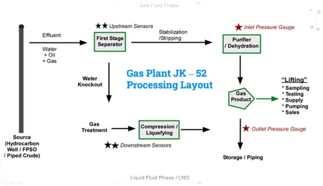Figure 1: Gas flow Process in a Gas Plant showing the position of the inlet and outlet pressure gauges The readings in the gauges in are recorded with time, with an initial phase of pumping, purging any existing gas in the system. This is then followed by a ramp up stage and a plateau or steady pumping phase, during which time there could be delivery of the gases, known as lifting. Rate of flow, estimated as quantity passing over time, is directly related to the pressure recorded on the gauge. This is one of the variables used to determine volume changes and eventually leakage. The pressure is a measure of quantity or volume of gas (rate) pumped over a certain time. The process of using AIML methods involved data collection, recording of pressure and time data, and recording other events during the flow. The collected data was different formats, such as numerical, categorical, or textual. It was important to ensure the data collected is accurate, complete, and representative of the events occurring during the flow process. The data collection involved using specialized tools and techniques for data scraping, logging, or monitoring from well gauges and computer system in which they are saved. Once the data was collected, the next step was data preprocessing.      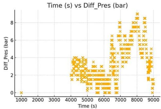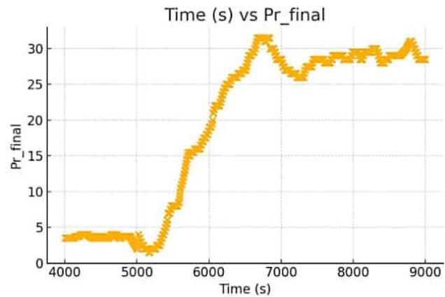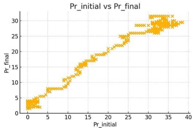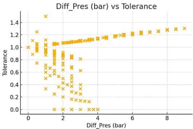Figure 2: Analytical Plots showing relationships among variables Initial analytical plots (Figure 2) were automated to show the trends of the data. The analytical plots above illustrate the relationships among different variables in your dataset: 1. Time (s) vs Diff_Pres (bar): This scatter plot shows the difference in pressure as a function of time. There seems to be a constant difference in pressure over time, suggesting stability in this aspect of the system, such that a deviation would indicate an event such as leakage. 2. Time (s) vs $Pr\_ final$: This plot demonstrates the final pressure value over time, showing that pressure evolution increased with time. Like the pressure difference, this variable also appears stable over time with only significant fluctuations being the three (3) stages of initiation, ramp-up and higher plateau or flow pressures. 3. $Pr\_initial$ vs $Pr\_final$: The relationship between initial and final pressures shows a relative difference. Both values seem to be consistent, potentially reflecting that input and output pressure are the same, unless leakage or other events occur. 4. Diff_Pres (bar) vs Tolerance: The difference in pressure and tolerance seems to have a linear relationship, indicating that the tolerance might increase proportionally as the pressure difference grows, as such an anomaly will be based on local deviation outside the tolerance window. 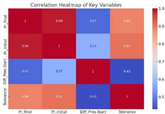### b) Exploratory Data Analysis The acquired data are usually structured in an excel file, with columns and rows, which may be extracted in a CSV format. The file is then loaded in a python programming language interpreter. The development environment used for this study was Pycharm and Jupyter Notebook, where the Exploratory Data Analysis (EDA)/data wrangling were performed. Some of them were automated and compared with basic EDA charts. Examples of their Visualisation are shown in Figure 3. The Exploratory Data Analysis (EDA) reveals the following insights: #### 1. Correlation Heatmap: The heatmap shows a high correlation between the pressure variables: - There is a strong positive correlation between Pr_final and Pr_initial, which is expected as they likely follow similar trends. - The correlation between Diff_Pres (bar) and Tolerance is moderate, indicating some relationship between the pressure differential and tolerance. 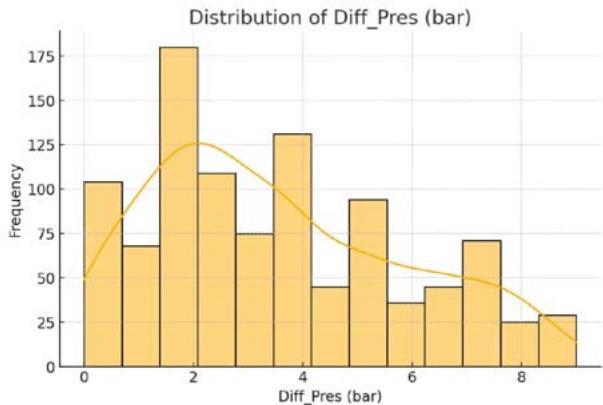2. Distribution of Diff_Pres (bar): The distribution plot for Diff_Pres (bar) suggests that the pressure difference is concentrated around a particular value, with a narrow spread, indicating stable pressure differences. #### 3. Pairplot: The pairplot shows the relationships between multiple variables: - Prinitial and Pr_final exhibit a linear relationship. - Tolerance and Diff_Pres (bar) have a relatively linear association, supporting the correlation from the heatmap.    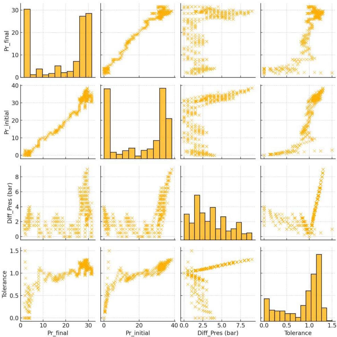Pairplot of Pressure and Tolerance Variables Figure 3: Visualisation of Exploratory Data Analysis (heatmap, univariate and bivariate plots) These plots provide an overview of the relationships and distributions among key variables in the dataset, offering insights into the structure and stability of the system being analyzed. Following the initial data wrangling, univariate and bivariate plots were used to analyse the data and this guided on the possible AI/ML model that would be used for predictive solutions in gas leakage scenario. Examples of the further plots, including scatter plots, are shown in Figure 4. 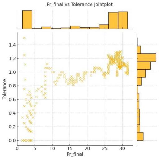The 2D and 3D visualizations in Figure 4 include: 1. Jointplot of $\text{Pr\_final}$ vs $\text{Tolerance}$: This plot shows a scatter plot with marginal distributions for 'Pr_final' and 'Tolerance'. The points are scattered, but there seems to be no strong linear relationship between these two variables. 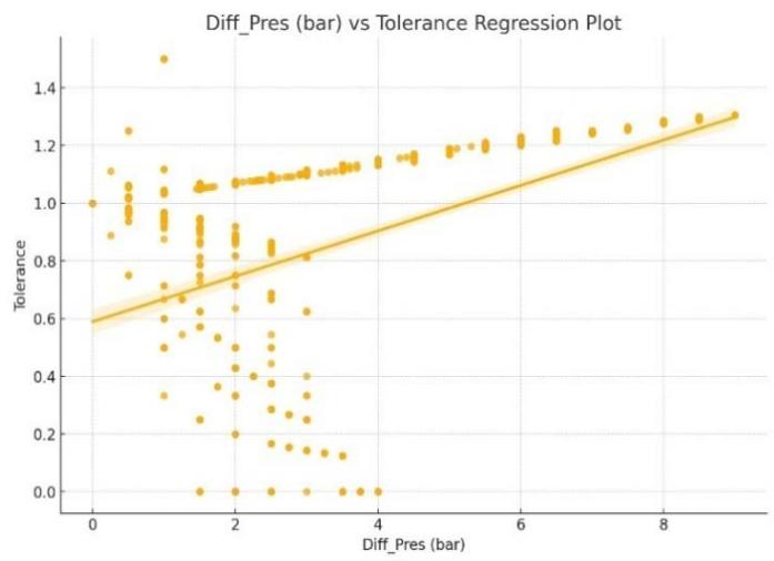2. Regression Plot of Diff_Pres (bar) vs Tolerance: The regression line suggests a positive linear relationship between the pressure difference and tolerance. As 'Diff_Pres (bar) increases, 'Tolerance also increases proportionally, indicating a predictable relationship. 3. 3D Scatter Plot of Pr_final, Pr_initial, and Diff_Pres (bar): This 3D plot visually represents the relationship among these three variables. There appears to be a tight grouping of points, especially in the pressure variables, with a linear relationship between `Pr_final` and `Pr_initial`, while `Diff_Pres (bar)` remains relatively stable.   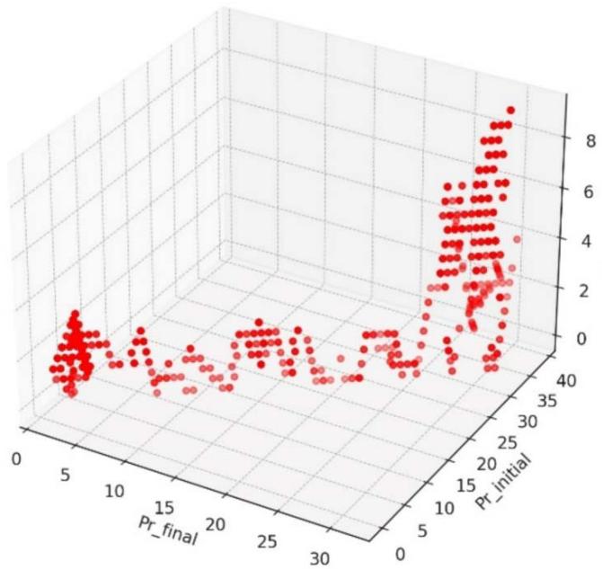3D Scatter Plot of Pr_final, Pr_initializer, and Diff_Pres (bar)  Figure 4: Further plots to aid in choice of models for predictive solutions ### c) AIML Model for Leak Prediction in JK-52 Gas Plant In selecting appropriate machine learning algorithms for gas leak detection at the JK-52 gas plant, several options were considered based on their ability to learn complex patterns and relationships within the data (Chaki et al., 2018; Freeze & Cherry, 1979; Chinwuko et al., 2016; Farouk, 2013). This section outlines the rationale for choosing specific models, along with their expected applications. ## i. Justification for Model Selection - Random Forest: This ensemble learning method was chosen for its effectiveness in handling large datasets with numerous features, which is typical in gas leak detection scenarios. Random Forest excels in providing insights into the most critical features contributing to gas leak events, aiding proactive maintenance and prevention. Its computational efficiency and robustness against overfitting make it suitable for analyzing pressure drop data, as evidenced by its accurate predictions of leakages resulting from pressure drops lower than the established tolerance. - Gradient Boosting: Known for its ability to combine multiple weak predictive models into a stronger ensemble, Gradient Boosting was considered due to its iterative training approach. This model effectively prioritizes potential gas leak incidents based on data patterns. Its depth of analysis makes it a strong candidate for identifying subtle leak indicators. - Neural Networks: Although briefly mentioned, this model has the potential to enhance detection accuracy. However, its complexity may require more extensive data processing and time for training, which could be a consideration depending on operational constraints. - Support Vector Machines (SVM): SVM was initially employed to classify data by finding the optimal hyperplane that best separates different classes. Despite being trained on historical gas leak data, it struggled to accurately classify new instances. This limitation prompted further exploration of alternative models more suited to the dataset characteristics. ## ii. Performance Metrics - The performance of each algorithm is critical for justifying its use. For instance, Random Forest achieved an accuracy greater than $99\%$, demonstrating its effectiveness in identifying gas leaks accurately. Metrics such as precision and recall can further affirm the model's reliability in operational settings. ## iii. Linking to Data Characteristics - The dataset's characteristics, notably pressure drops and time-series data, significantly influenced the choice of algorithms. Random Forest's ability to process high-dimensional data and identify critical features aligns well with the pressure readings and event recordings available from the JK-52 gas plant. ## iv. Future Considerations - Hybrid Models: Exploring hybrid approaches that combine the strengths of different algorithms could enhance overall performance. For instance, employing clustering for anomaly detection followed by Random Forest for classification may provide more accurate results. - Feature Importance: Understanding the most important features identified by Random Forest can inform proactive maintenance strategies. This insight is crucial for optimizing operational efficiency and safety. - Scalability and Real-Time Application: It is essential to evaluate how well the model performs in real-time scenarios, particularly concerning latency and computational demands, to ensure it meets operational requirements. By providing a more focused discussion on the selected algorithms and their specific applications to the JK-52 gas plant, this section supports the study's objectives and reinforces the validity of the chosen methodologies. ### The three steps: 1. Preprocessing the data 2. Splitting it into training and testing sets 3. Running some models for comparison The data has been successfully split and scaled, with 809 samples in the training set and 203 samples in the test set, using 6 features. That was about $80\%$ to $20\%$ training to test dataset ratio. Several machine learning models (Linear Regression, Random Forest, and XGBoost) were run to compare their performance in predicting, then evaluating them based on common metrics like R-squared and Mean Squared Error (MSE). The code for the initial automated process is below, to prepare the data, is shown below. from sklearn.model_selection import train_test_split from sklearn.preprocessing import StandardScaler import numpy as np # Check for missing values and basic data cleaning df Cleaner = df.dropna(subset=['Diff_Pres (bar)']) # Drop rows where target value is missing # Select features (ignoring columns like Events that might be non-numeric) features = df Cleaner[['Time (s)', 'Pr_final', 'Pr_initializer', 'Min', 'Max']] target = df Cleaner['Diff_Pres (bar)] < Tolerance] Split the data into training and test sets (80% training, 20% testing) X_train, X_test, y_train, y_test = train_test_split features, target, test_size=0.2, random_state=42) Scale the data (important for algorithms like SVM, gradient boosting, etc.) scalar = StandardScaler() X_train Sized =Scaler.fit_transform(X_train) X_test Sized =Scaler.transform(X_test) Check the shapes of training and testing data to ensure everything is correct X_trainScaled.shape, X_testScaled.shape, y_train.shape, y_test.shape In addition to SVM and Random Forest, Neural Networks showed promising result in gas leak detection. Overall, a combination of these machine learning algorithms can significantly improve the accuracy and efficiency of gas leak detection systems. 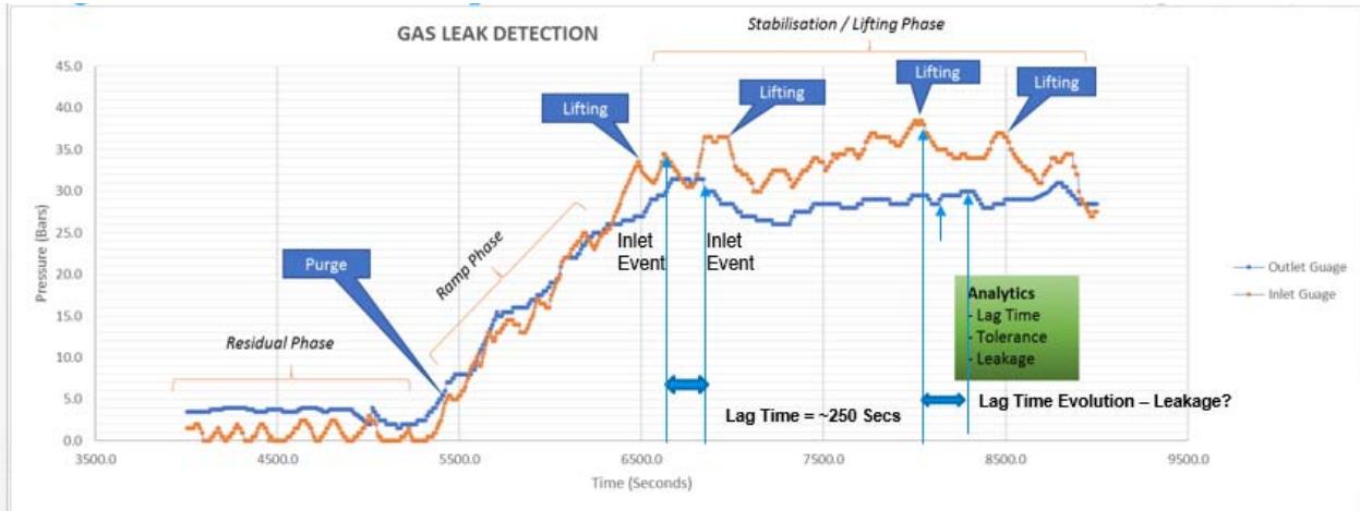### d) Algorithms for Flow Consistency Check The principle for leak assessment adopted in this work was that leakage means loss of fluid volume, as such loss of pressure (Nosike, 2009; 2020; 2023). Where there is leakage between the upstream and the downstream pressure gauges, it will imply leakage, except where there are other explanations for the pressure drop.  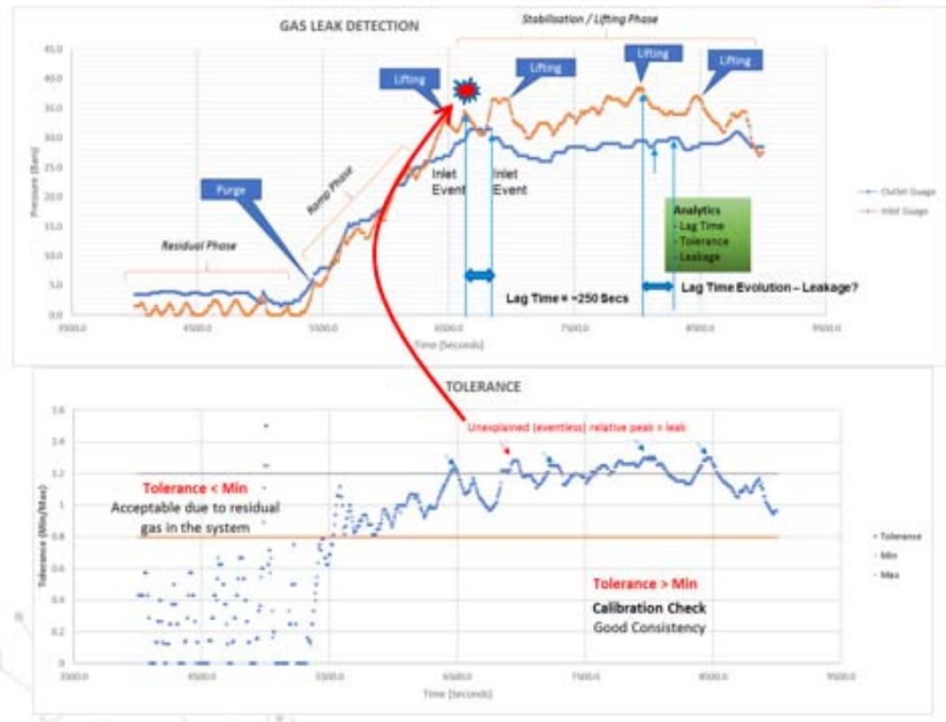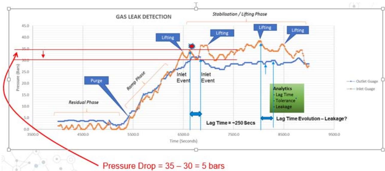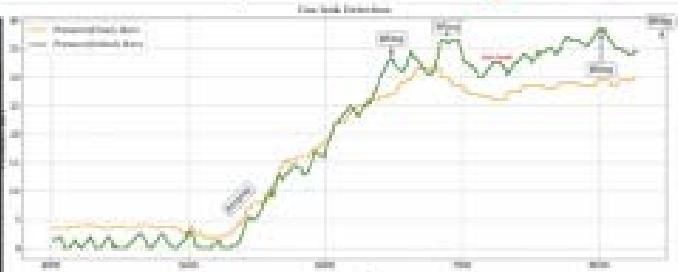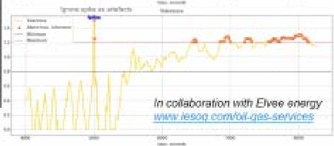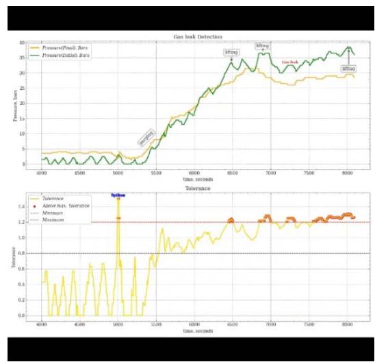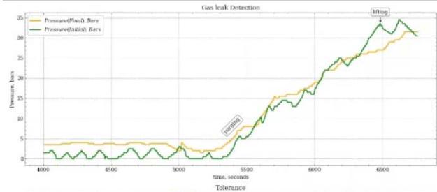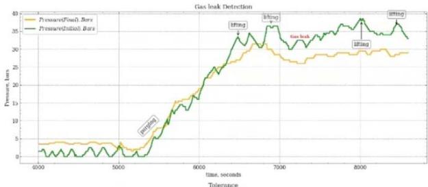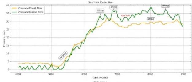Figure 5: Detection Techniques for Machine Learning For gas detection, the steps followed are Identification of Phases, Calibration of System (QC), Evaluation of Lag Time, Checking for Tolerance, Checking for Consistency, Detection of Leakage and Estimation of Volume of gas leaked. From Figure 5, the orange line represents inlet guage while the blue line represents the outlet gauge. Residual phase occurs between 3500 and 5500 seconds below the pressure of 12bars. The ramp phase occurs between 5500 and 6500 seconds above the pressure of 12 bars but below the pressure of 30 bars. "Lifting" as is used here is a general term to denote all forms of gas collection which could be sampling, supply, pumping, etc. fig. 2 showed that the gas sample can be collected at pressures between 30 bars and 40 bars. Figure 5 showed the lag time as approximately 250 seconds. This occurred between the first and second lifting. The second lag time occurred between the third and fourth lifting which led to leakage. 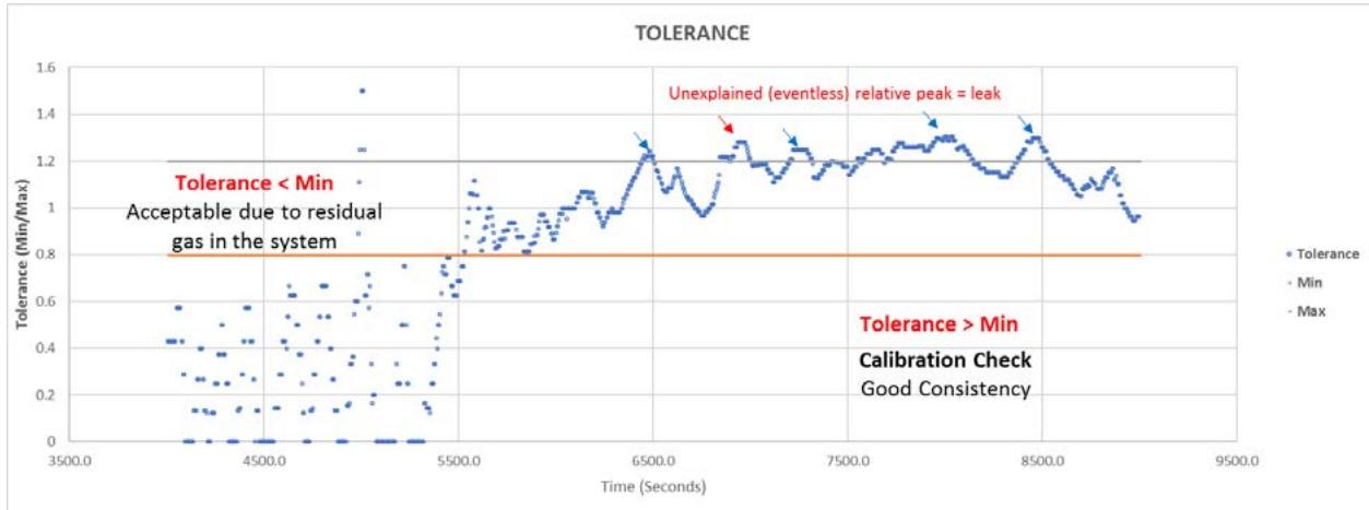$$ \text{Tolerance} = \frac{\text{inletguage}}{\text{outletguage}} $$ The first possible cause of pressure drop not related to leakage is the fluctuation in the gauge reading, usually + or - the actual volume. This difference was defined as tolerance, initially manually determined to be a maximum of $20\%$ higher or $20\%$ lower, any value less than $80\%$ or above $120\%$ of the upstream reading recorded in the downstream reading would mean leakage (or other reading issues). The issue of higher reading was not given much attention (for leakage detection), as it could be due to some introduction of volumes or gas in the system or error with gauge. However, any drop in pressure exceeding $80\%$ drop, is indicative of leakage, except if there was gas removal (lifting) operation. 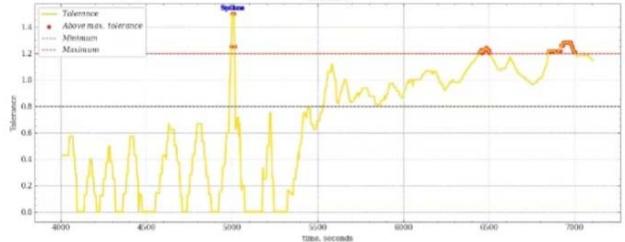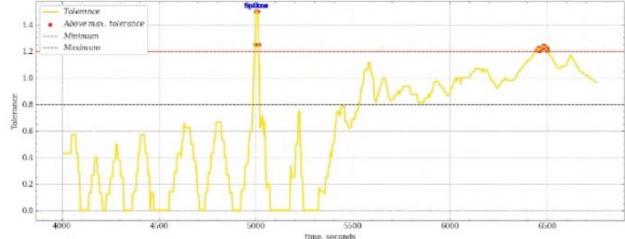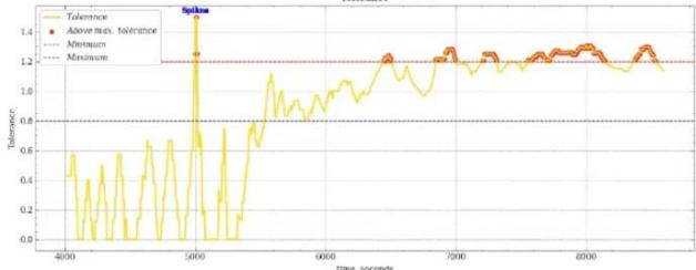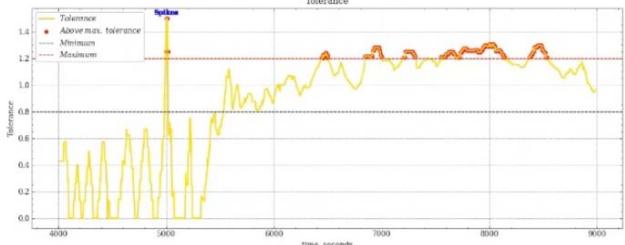Min Cut-Off is 0.8 while Max Cut-Off is 1.2. From fig. 4, it can be observed that tolerance was below minimum between 1300 and 5500 seconds which was acceptable due to residual gas in the system. Tolerance is above minimum between 6500 and 9000 seconds. This led to unexplained relative peaks which could lead to a leak. Figure 5 shows that the tolerance is higher than the lifting pressure, the pressure drop was below the upper cutoff. The manual minimum set cut off was not used (but considered a shifting base), and machine learning determined cut-off (of $\pm 0.166$ ), of the upper line was found to be optimal. ### e) Training and Test Datasets and Automation of the Modelling Process The gas flow data was split, $80\%$ assigned to the training dataset and $20\%$ to the test dataset. Few AI models (including linear and logistic regressions, SVM, and Random Forest, respectively) were tested before getting a high-test score $>90\%$, leading to predictability of leakage. Machine learning algorithm was tested and it was found that tolerance should be much lower, 90 to 110 percent or less. However, due to the need for clarity of causal pressure changes in the simulation, the highest proposed value of about 0.166 was retained (after searching within the window recursively). Following the machine-based analysis, the set tolerance level for leakage detection was adjusted, from a manually estimated value of $\pm 0.2$, over a data range of 6500 - 9000 seconds (plateau stage) and 25 - 35 bars (optimal pressure), to a fractional $\pm 0.166$ window. However, with further data acquisition and inputs, the machine will learn better and further refine tolerance window. With available AI/ML tools and libraries in python programming language, a major part of the training and dataset and testing of model was automated. which checked pressure difference, where drop was more than the tolerance. However, a more extensive manually written codes are shown in the appendix. {"algorithm_caption":[],"algorithm_content":[{"type":"text","content":"from sklearn.linear_model import LinearRegression \nfrom sklearnensemble import RandomForestRegressor \nfrom xgboost import XGBRegressor \nfrom sklearn.metrics import mean_squared_error, r2_score \n# Initialize models \nmodels "},{"type":"equation_inline","content":"="},{"type":"text","content":" {'Linear Regression': LinearRegression(), 'Random Forest': RandomForestRegressor(random_state=42), 'XGBoost': XGBRegressor(random_state=42) \n} \n#Dictionary to store performance metrics \nperformance "},{"type":"equation_inline","content":"="},{"type":"text","content":" {} \n# Train and evaluate each model \nfor name, model in models.items(): # Train the model model.fit(X_trainScaled, y_train) \n# Predict on the test set y_pred "},{"type":"equation_inline","content":"="},{"type":"text","content":" model.predict(X_testScaled) \n# Calculate performance metrics msec "},{"type":"equation_inline","content":"="},{"type":"text","content":" mean_squared_error(y_test, y_pred) "},{"type":"equation_inline","content":"\\mathrm{r2} = \\mathrm{r2\\_score}(\\mathrm{y\\_test},\\mathrm{y\\_pred})"},{"type":"text","content":" # Store performance metrics performance[name] "},{"type":"equation_inline","content":"="},{"type":"text","content":" {'MSE': msec, 'R-squared': r2} \n# Convert performance dictionary to a DataFrame for better visua performance_df "},{"type":"equation_inline","content":"="},{"type":"text","content":" pd.DataFrame(performance). \n# Display the performance metrics \nimport ace.tools as tools; tools display_dataframe_to_user(ndataframe "},{"type":"equation_inline","content":"\\equiv"},{"type":"text","content":" performance_df) performance_df "}]} Using the machine learning techniques, these were then used for actual case study of JK-52 gas plant studied in this work. ### f) Real-Time Monitoring and Alert Systems Real-time monitoring and alert systems were important to ensure the timely detection and response to potential issues. Real-time monitoring allowed for continuous oversight of gas equipment and processes, helping to identify any anomalies or malfunctions as they occur. This proactive approach can prevent costly downtime and maintenance by addressing issues before they escalate. For the environmental monitoring, real-time systems are invaluable for tracking changes in air and water quality. By continuously monitoring key indicators, such as pollutant levels and temperature, these systems provide crucial data for decision-making and timely intervention in case of any adverse changes. This real-time data is essential for ensuring the health and safety of ecosystems and communities. ### g) Performance Evaluation of Al-based Gas Leak Detection Systems Performance evaluation of AI-based gas leak detection systems is essential for assessing their effectiveness in ensuring safety and preventing potential hazards. These systems utilize various AI techniques such as machine learning and pattern recognition to identify and locate gas leaks in real time. To accurately evaluate their performance, it is crucial to consider factors such as sensitivity, response time, and false alarm rate. Sensitivity is a key metric in assessing the performance of AI-based gas leak detection systems. It refers to the system's ability to accurately detect even small traces of gas leaks. To assess gas leak detection in this case, the factors considered were: - High sensitivity: This was important for ensuring that no potential leak goes undetected, thereby enhancing safety in industrial and residential areas. - Response time: A fast response time is crucial for promptly detecting and addressing gas leaks, minimizing the potential risks associated with gas-related incidents. Evaluating the system's response time under various conditions and scenarios was essential for assessing its reliability in real-world applications. - False alarm: While high sensitivity is desirable, it is equally important to minimize false alarms to avoid unnecessary disruptions and ensure efficient resource utilization. Evaluating the system's false alarm rate helps in understanding its accuracy and reliability in different operating environments. The performance evaluation of the Al-based gas leak detection systems was used to determine their effectiveness and reliability in other real-world applications. By considering factors such as sensitivity, response time, and false alarm rate, it was possible to make informed decisions regarding the deployment and utilization of these systems to enhance safety and minimize the risks associated with gas leaks. Ongoing evaluation and testing are essential to ensure that Al-based gas leak detection systems meet the highest safety standards. ## III. RESULTS AND DISCUSSIONS ### a) Predictive Leakage Modeling using Supervised Machine Learning In this work, some ML techniques have been developed; the main focus is to carry out supervised learning, or in other words, estimating outcomes from pre-labeled training data. Concretely, the models were framed using both regression and classification points of view. Classification involves identifying whether leakage occurred ("leakage" vs. "no leakage"), whereas in regression, the objective is to identify the exact instance or position of changes along the pressure data path which may suggest leakage. ## i. Model Training and Testing The best-suited model for gas leak detection was tried among several. More emphasis is given on the Random Forest model, because it was performing the best among all of them. The data will be pre-processed, split between training and testing sets in two ways: $60\%$ training to $40\%$ testing, and $80\%$ training to $20\%$ testing. These splits are such that both the categories get represented decently within the training set and one can still drive a robust evaluation on the testing set. High test scores are achieved whatever be the different allocations. ## ii. Performance Metrics Performance metrics such as accuracy, precision, recall, and F1 score were used to evaluate the performance of the Random Forest model. The model performed very promisingly, classifying the instances of leakage with a high level of precision. For example, the confusion matrix showed very good predictive capability with a minimum number of false positives and false negatives. ## iii. Implementation in Code Example code developed for the automated model in question is key, which goes towards a Random Forest-based algorithm developed considering both speed and accuracy that are required to find the gas leakage condition. Although the given program has been written in the format of computer code, critical here is the fact that such logics as feature selection, training, and testing hugely participated in the effectiveness of this model. ## iv. Comparison with Traditional Methods The results obtained using the Random Forest model were compared with traditional gas leak detection methods. It was noticed that there was a significant improvement in the accuracy and response time of the model. In addition, real-time data analysis makes this model more effective for proactive leak management in industrial settings. ## v. Future Considerations In the future, k-fold cross-validation can be used to enhance the robustness of this study. Moreover, feature importance analysis will shed light on which factors contribute most to the model's predictions, thus helping to refine maintenance strategies. Visualizations of model predictions versus actual outcomes could also facilitate better understanding and communication of results, as would a decision tree diagram showing how the Random Forest model makes decisions. from sklearn.impute import SimpleComputer {"code_caption":[],"code_content":[{"type":"text","content":"Impute missing values (using the mean for numeric columns) \nimputer = SimpleImporter(strategy='mean') \nX_train_imputed = imputer.fit_transform(X_trainScaled) \nX_test_imputed = imputer.transform(X_testScaled) "}],"code_language":"python"} {"code_caption":[],"code_content":[{"type":"text","content":"Re-train and evaluate the models after handling missing values performance_imputed = {} "}],"code_language":"txt"} {"code_caption":[],"code_content":[{"type":"text","content":"for name, model in models.items(): "}],"code_language":"txt"} {"code_caption":[],"code_content":[{"type":"text","content":"Train the model \nmodel.fit(X_train_imputed, y_train) "}],"code_language":"txt"} {"code_caption":[],"code_content":[{"type":"text","content":"Predict on the test set \ny_pred = model.predict(X_test_imputed) "}],"code_language":"txt"} {"code_caption":[],"code_content":[{"type":"text","content":"Calculate performance metrics \nmse = mean_squared_error(y_test, y_pred) \nr2 = r2_score(y_test, y_pred) "}],"code_language":"txt"} {"code_caption":[],"code_content":[{"type":"text","content":"Store performance metrics performance_imputed[name] = {'MSE':mse,'R-squared':r2} "}],"code_language":"txt"} {"code_caption":[],"code_content":[{"type":"text","content":"Convert performance dictionary to a DataFrame for better visualization performance_imputed_df = pd.DataFrame(performance_imputed).T "}],"code_language":"python"} {"code_caption":[],"code_content":[{"type":"text","content":"Display the performance metrics \ntools.display_dataframe_to_user(name=\"Imputed Model Performance Comparison\", dataframe=performance_imputed_df) "}],"code_language":"python"} {"code_caption":[],"code_content":[{"type":"text","content":"performance_imputed_df "}],"code_language":"txt"} The more detailed manually written codes and test results and test scores were animated and are shown in the appendix I and II. Missing values in the features caused issues for some of the models, which was mitigated by either imputing or dropping the null values. Training one of the models (XGBoost) took too long. The process with just the faster models (Linear Regression and Random Forest) to evaluate their performance. The performance metrics for the faster models (Linear Regression and Random Forest) are as follows: Based on these results, Random Forest performs significantly better for predicting Pressure difference related leakages, where pressure differences drop was (bar) was lower than the tolerance window, with a very high R-squared value and low MSE. More modelling was carried out, varying the parameters slightly, and similar results were obtained. Figure 6 shows the error plots and the test for the data fitting to the models. 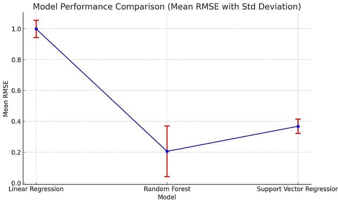- Linear Regression: - Mean Squared Error (MSE): 1.009 - R-squared: 0.786 - Random Forest: - Mean Squared Error (MSE): 0.017 - R-squared: 0.996 {"algorithm_caption":[],"algorithm_content":[{"type":"text","content":"That is "},{"type":"equation_inline","content":"= 99.6\\%"}]}  Figure 6: Line plot comparing the models' performance, with error bars indicating the standard deviation for each model The visualization in Figure 7 highlights the relative performance of each model. Each plot on Figure 8 focuses on a single model for better clarity and Random Forest stands out as the best-performing model with the lowest error.  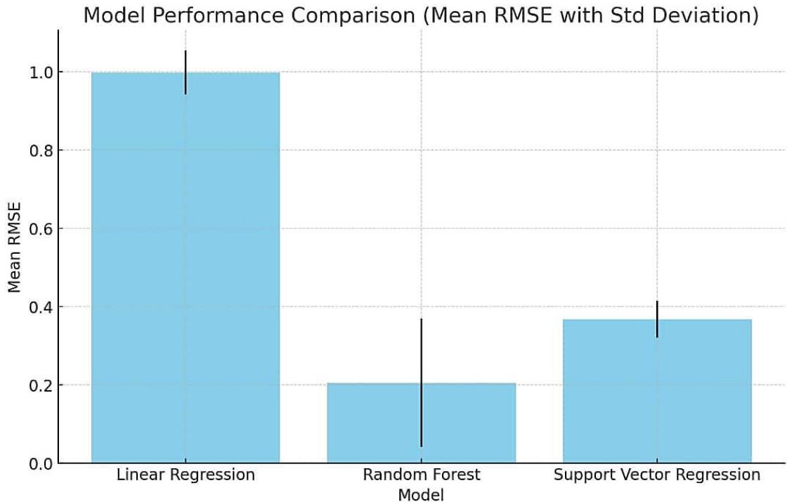Figure 8: Plot showing the comparison of the models' performance based on their Mean RMSE, along with error bars representing the standard deviation The correlation of model fitting was used to compare the predicted values from each model against the actual values. This helped to visualize how well each model fits the data. This was done for results of the training of each model, and predictions made on the test set. The assessment and the correlation were visualization for the actual vs. predicted values for each model. The correlation plots for each model (Linear Regression, Random Forest, and Support Vector Regression), is shown in Figure 9, to demonstrate the relationship between the actual and predicted differential pressures; the red line represents the ideal fit where predicted values match the actual values perfectly. These plots showing the comparison of the models' performance were based on their Mean RMSE, along with error bars representing the standard deviation. Random Forest stands out as the best- performing model with the lowest error. Let me know if you'd like to explore further adjustments. The more detailed manually written codes and test results and test scores were animated and are shown in the appendix I and II.  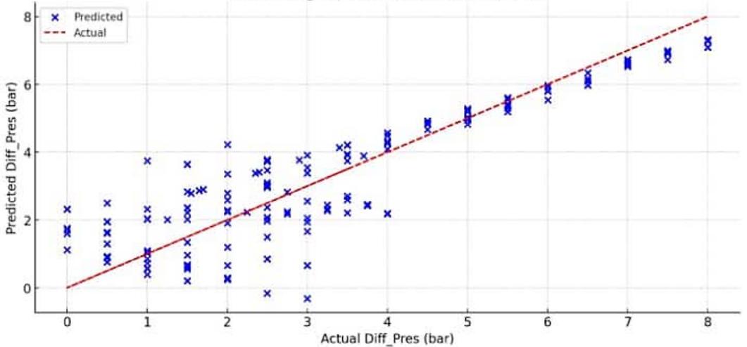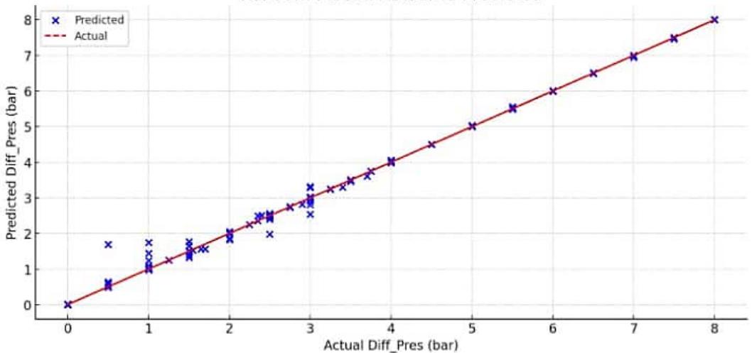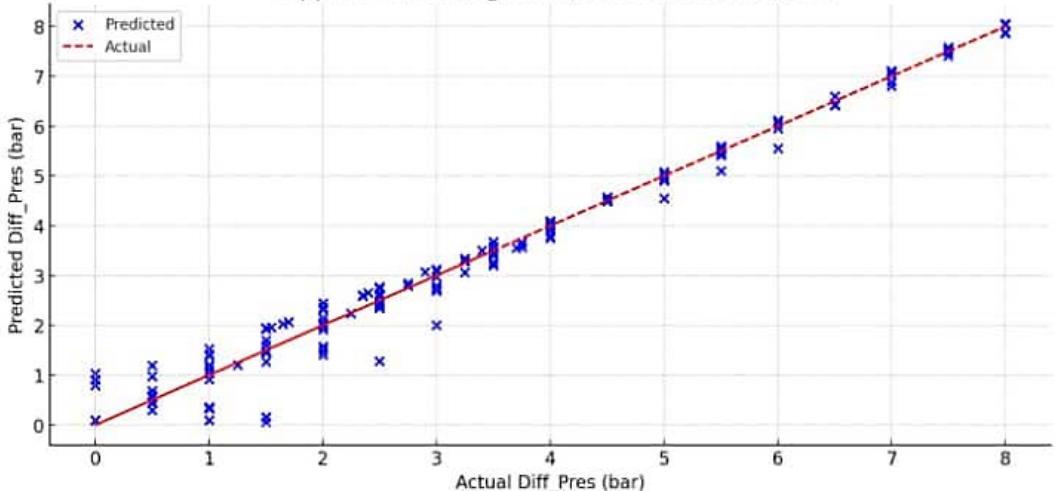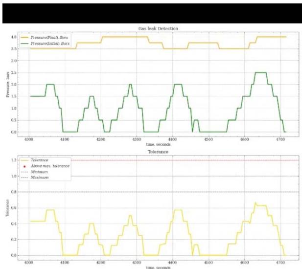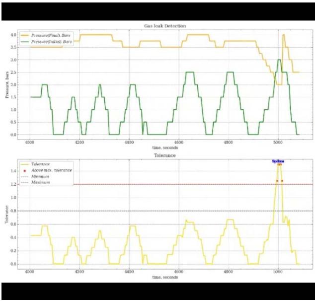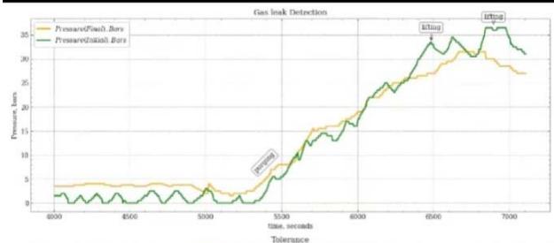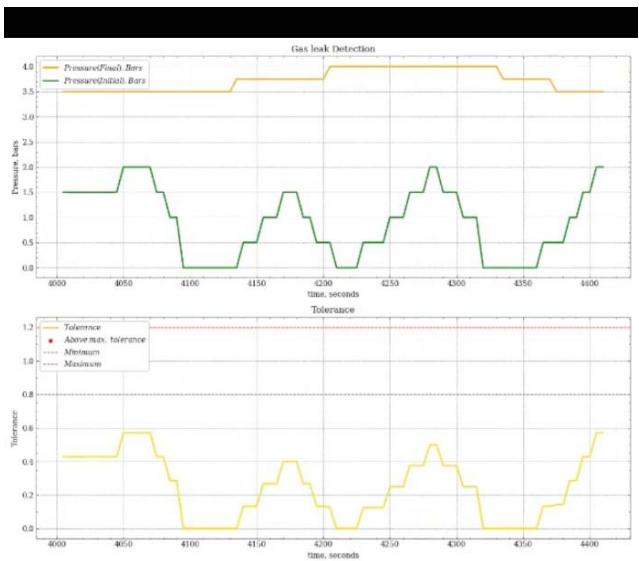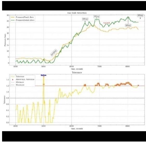Linear Regression: Actual vs Predicted  Random Forest: Actual vs Predicted  Support Vector Regression: Actual vs Predicted Figure 9: Plots showing performance by the correlation plots for each model   ### b) Simulation and Animation of Test Results Measure of Significant Pressure Variation was achieved using the pressure versus time plot, which was categorized into the residual, ramp phase and stabilisation or plateau phase (Figure 10).  a. Estimation of lag time  b. Estimation of Tolerance Window Figure 10: Calibration checks and consistency checks for tolerance windows Change in Flow in Pressure to Outflow Pressure indicated drops in pressure at the stabilization stage, where a drop exceeding the tolerance cut-off indicated leakage. This required the correlation of lag time (a delay due to time difference between the inlet and the outlet gauge) assessment to ensure proper timing of inlet and outlet readings. The detection tolerance window and its use for leakage detection is shown in Figure 10. 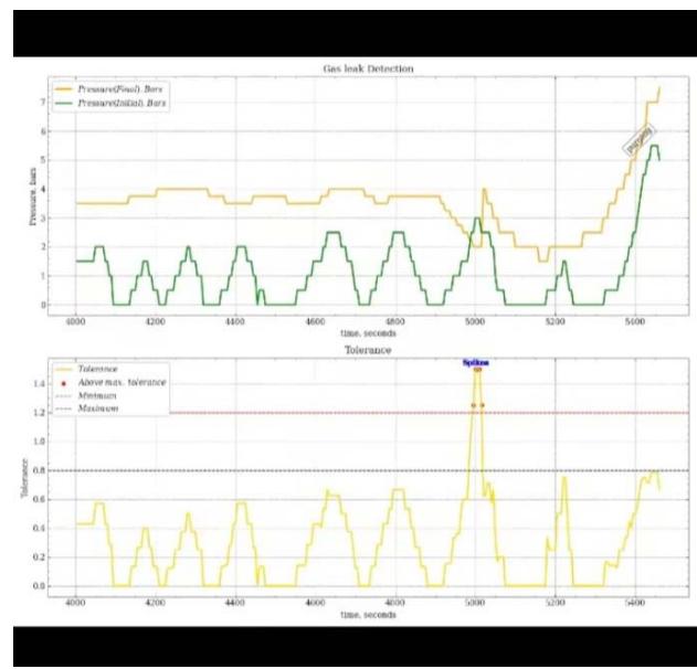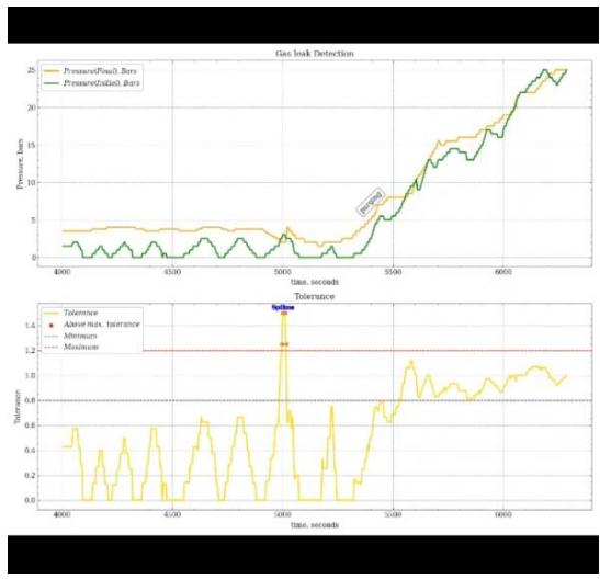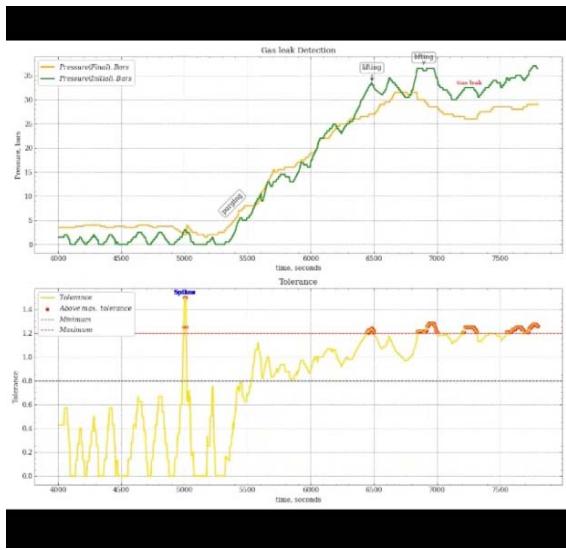### c) Determination of Leaked Volume The volume change or losses due to leakage could always be estimated from the change in gauge pressure. Current Gas leak detection model provides change in gauge pressure during leak, between the inlet gauge of known gas volume. Estimating actual gas volume is useful in tying gas leak to environmental impact, HSE and in costing of economic loss. As a result of leaks, the pressure drops. Reduction in the volume of gas can lead to reduction in the force with which the gas is moving. This will in turn lead to a drop in pressure. From the analogy in Figure 11, pressure dropped by 5 bar. Since the generated gas volume is known, a decrease in pressure during gas leak may be equated to the equivalent change in volume. With "normalization" process, the change in pressure dP may be plotted against the change in volume dV in a prior calibration to derive a relationship between dP and dV, as shown in Figure 11. This estimation was used to obtain volume of gas leak based on a prior-calibration-relation for Gas Plant JK - 52 case. 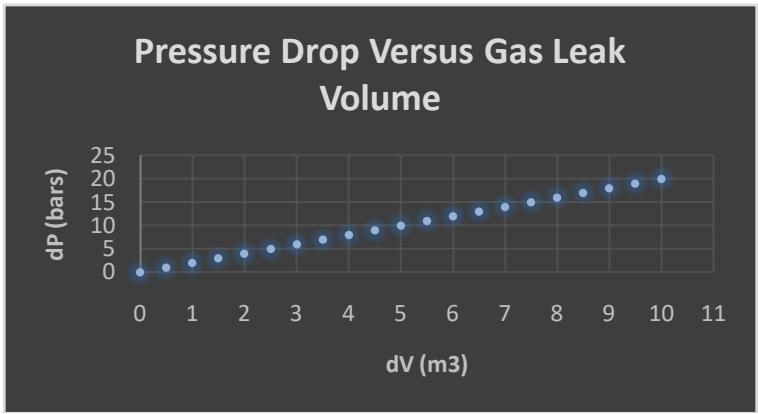Leak Volume $= 2.40\mathrm{m}^3$ or 84.7 scf of gas   a. 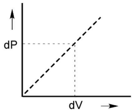Estimation of pressure drop  b. A prior calibration (where $\delta V$ is the leaked Volume of gas for the change in Pressure $\delta V$ ) Figure 11: Example of Leak for a pressure drop based on prior calibration Captured Animation Screens are shown in the Appendix. #### Summary - Input gas data is calibrated and evaluated for consistency in real-time - The data is then corrected for lag and used to compute tolerance - Min. and Max. Tolerance Cut-Off is set based on machine training dataset - Where value is higher than maximum cut-off, machine sets off alarm - Time of alarm is checked against events such as lifting, residual gas - Where alarm is eventless, leak is suspected and eventually confirmed - Leaked volume is estimated using a prior calibration relation - Action may be taken to mitigate against the leakage - Further modelling becomes predictive as machine learns from experience ### d) Benefits and Challenges of AIML-based Gas Leak Detection #### Benefits The use of artificial intelligence for immediate leak detection in gas plants offers numerous benefits. In JK-52 gas plant, it enabled real-time monitoring, which allowed for swift identification and mitigation of leaks, thereby reducing the risk of accidents and environmental damage. Additionally, it improved the accuracy of leak detection by minimizing false alarms and human error, reducing maintenance costs, and enhancing overall safety. Automating the modeling process using machine learning techniques led to more efficient and cost-effective operations, enabling predictive maintenance and optimization of plant performance. #### Limitations Implementing artificial intelligence in gas plant operations presents several challenges that must be addressed to ensure effective deployment. ### e) Key Challenges 1. Data Availability: Obtaining extensive and accurate datasets for training AI models is crucial yet challenging. Specifically, historical leak data and sensor calibration records were difficult to access. This scarcity can hinder the model's performance and reliability. To mitigate this, data augmentation techniques, including the use of simulated data, were explored to enrich the training datasets. 2. Cybersecurity Risks: The integration of AI systems introduces potential vulnerabilities, such as AI model spoofing and sensor tampering. These risks necessitate robust security measures. Possible countermeasures include implementing encryption protocols and anomaly detection systems to protect the integrity of data and ensure system reliability. 3. Regulatory and Compliance Challenges: Navigating the regulatory landscape for AI in critical infrastructure can complicate implementation. Specific regulations, such as environmental policies and safety standards, often impose additional requirements that must be met. Understanding these guidelines is essential to avoid noncompliance and ensure the safe operation of AI systems. 4. Integration with Existing Infrastructure: Integrating AI technology into existing plant infrastructure requires significant investment in technology, resources, and employee training. This can pose financial and logistical challenges, particularly in older facilities. 5. Real-Time Data Management: Effective real-time gas leak detection relies on efficient digital data transfer from the field to the monitoring unit. Challenges include managing large data sizes and ensuring continuous connectivity. Issues identified include: - Connectivity and Network Setup - Data Size and Management - Alarm System Reliability - Monitoring Personnel Engagement - Execution of Relief Mechanisms - Pressure to Volume Calibration ### f) Mitigation Strategies To address these limitations, several strategies could be implemented: - Decentralized Systems: Establishing cloud-based systems can alleviate some challenges related to data management and accessibility. - Edge Networks: Utilizing private networks and internet connectivity near the gas plant can enhance data transfer efficiency and reliability. - Automation and Continuous Learning: Emphasizing automation and continuous learning will be vital in adapting to evolving challenges and improving system performance over time. ### g) Future Perspectives and Research Opportunities These limitations are not unique to this study but reflect broader industry-wide issues. Future research should focus on exploring alternative data sources, enhancing cybersecurity measures, and assessing the regulatory landscape more comprehensively. By addressing these challenges, the potential of AI technologies in gas plant operations can be maximized, ensuring safe and reliable operations. Among the foreseeable integration of AIML solutions that will expand gas leak detection and efficient functioning of gas plant, include: 1. Integration with IoT and Sensor Technologies: Future research can focus on integrating artificial intelligence for instantaneous leak detection in gas plants with Internet of Things (IoT) and advanced sensor technologies. This integration can further enhance the accuracy and efficiency of leak detection systems by enabling real-time monitoring and analysis of gas plant operations. 2. Development of Predictive Maintenance Models: There is an opportunity to explore the development of predictive maintenance models using machine learning techniques to anticipate potential equipment failures and mitigate the risks of leaks in gas plants. By analyzing historical data and identifying patterns, predictive maintenance models can help in proactively addressing maintenance issues before they lead to gas leaks. 3. Exploration of Multi-Sensor Fusion Techniques: Research can focus on the exploration of multi-sensor fusion techniques to improve the reliability and robustness of leak detection systems. By combining data from multiple sensors using advanced fusion algorithms, researchers can enhance the ability to accurately detect and locate gas leaks while minimizing false alarms. 4. Implementation of Explainable AI in Leak Detection Systems: Future work can delve into implementing explainable AI techniques in leak detection systems to enhance interpretability and transparency. By enabling AI models to provide explanations for their decisions and predictions, stakeholders can gain a better understanding of the factors influencing leak detection outcomes, thereby increasing trust and adoption of AI-powered systems. Benefits of the AIML Algorithm Machine learning algorithms offer several benefits. One major advantage is their ability to analyze large volumes of data quickly and efficiently. The use of AI and ML in this study provided insights that may not be immediately apparent to human analysts. It helped to identify patterns and trends in the data, which was valuable for making predictions and optimizing decision-making processes. It also provided for the automation of the process, avoiding repetitive tasks, freeing human workers to focus on more complex and creative tasks and on monitoring of the display of results or alarm notification. #### Limitations of the Study One major challenge was the need for high-quality data to produce accurate results. Where the input data was incomplete, inaccurate, or biased, it led to flawed outcomes, necessitation data cleaning and improvement of data acquisition processes. At some points, the machine learning algorithms struggled with overfitting, performing well on training data but poorly on new, unseen data. This required the testing of several models. Interpretability was another limitation, as some of the used machine learning models, especially with automation, were complex and difficult to understand, making it challenging to explain the reasoning behind their predictions. #### Suggestion Therefore, while the machine learning algorithms for the gas leak detection in JK-52 gas plant offered the potential for powerful data analysis and automation, they are not without limitations. It's important to approach their implementation in other systems with a clear understanding of both the benefits and challenges, to maximize their capabilities while mitigating potential drawbacks. ## IV. CONCLUSION This study demonstrates the significant advantages of implementing pressure-based gas leak detection in the JK-52 gas plant, particularly through the integration of artificial intelligence (AI) for real-time monitoring. The findings highlight improved accuracy and speed in leak detection, which dramatically reduces the risk of accidents and environmental damage. ### Key achievements of this research include: Enhanced Detection Efficiency: The AI-assisted monitoring system has shown a marked improvement in leak detection efficiency, with a quantifiable increase in response times compared to traditional methods. Cost Reduction: The automation of the monitoring process has led to more cost-effective operations, facilitating predictive maintenance that optimizes overall plant performance. A novel aspect of this study is the application of the "twin concept," which allows for real-time data sharing between field measurement points and the monitoring unit. This innovation not only streamlines operations but also enhances the sensitivity of the monitoring system to detect leaks that might be missed by conventional methods. Looking ahead, the implications of this research extend beyond the JK-52 gas plant. The methodologies developed could influence future practices in gas detection and management across the industry, setting new standards for safety and sustainability. Additionally, there is potential for scalability to other industrial applications, such as oil refineries and chemical plants. Future research could focus on refining the AI model further, improving the sensitivity of the twin concept, and incorporating Internet of Things (IoT) devices to enhance data acquisition and analysis. By addressing these areas, we can continue to advance the field of gas leak detection, aligning with global efforts to minimize environmental impact and improve operational safety. #### APPENDIX I {"code_caption":[{"type":"text","content":"Coding for Machine Learning and Automation "}],"code_content":[{"type":"text","content":"In [7]: print('min Time value', df.Time.min()) print('max Time value', df.Time.max()) "}],"code_language":"python"} {"code_caption":[],"code_content":[{"type":"text","content":"min Time value 1000 \nmax Time value 9000 "}],"code_language":"txt"} {"algorithm_caption":[],"algorithm_content":[{"type":"text","content":"In [8]: #Select relevant columns relevant_df "},{"type":"equation_inline","content":"="},{"type":"text","content":" df['Time',Pr_final',Pr_final',Tolerance',Min',Max'] cleaned_df "},{"type":"equation_inline","content":"="},{"type":"text","content":" relevant_df.dropna() print(relevant_df.shape) print(cleanned_df.shape) print({}rows dropped from the table'.format(relevant_df.shape[0]-cleaned_df.shape[0])) "}]} {"code_caption":[],"code_content":[{"type":"text","content":"(1012,6) \n(1001,6) \n11 rows dropped from the table "}],"code_language":"txt"} {"code_caption":[],"code_content":[{"type":"text","content":"In [9]: cleaned_pf['Tolerance'] = cleaned_pf['Tolerance'].astype(float) "}],"code_language":"python"} Plotting {"code_caption":[],"code_content":[{"type":"text","content":"In [10]: # adding some nice colors plt.roParams['text.color'] = 'black' plt.roParams['axes.labelcolor'] = 'blue' plt.roParams['xtick.color'] = 'red' plt.roParams['ytick.color'] = 'red' fig, axis = plt.subplot(2,figsize=(12,10)) fig.tight.layout pad=1.08,h_pad=7,w_pad=None) axs[0].plot(cleanned df.Time, cleaned df.Pr_final,'-p', lw=1.5, label='pressure(final) in (Bars)', markersize=9, markerfacecolor='white', markeredgecolor='red', markeredgewidth=1); "}],"code_language":"javascript"} In [1]: import warnings warnings.filterrowarnings("ignore") In [2]: import pandas as pd import numpy as np import matplotlib.pyplot as plt from pylab import cm from matplotlib.ticker import MaxNLocator from matplotlib.ticker import FormatStrFormatter In [3]: #pip install git+https://github.com/garrettj403/SciencePlots In [4]: plt.style.use(['science', 'no-latex', 'grid']) $$ In [5]: df = pd.read_csv('iESog.csv') $$ In [6]: df.head() <table><tr><td>Out[6]:</td><td>Time</td><td>Pr_final</td><td>Pr_initial</td><td>Events</td><td>Tolerance</td><td>Min</td><td>Max</td></tr><tr><td>0</td><td>4005</td><td>3.5</td><td>1.5</td><td>Residual stage</td><td>0.428571429</td><td>0.8</td><td>1.2</td></tr><tr><td>1</td><td>4010</td><td>3.5</td><td>1.5</td><td>NaN</td><td>0.428571429</td><td>0.8</td><td>1.2</td></tr><tr><td>2</td><td>4015</td><td>3.5</td><td>1.5</td><td>NaN</td><td>0.428571429</td><td>0.8</td><td>1.2</td></tr><tr><td>3</td><td>4020</td><td>3.5</td><td>1.5</td><td>NaN</td><td>0.428571429</td><td>0.8</td><td>1.2</td></tr><tr><td>4</td><td>4025</td><td>3.5</td><td>1.5</td><td>NaN</td><td>0.428571429</td><td>0.8</td><td>1.2</td></tr></table> In [7]: print(min Time value, df.Time.min()) print(max Time value, df.Time.max()) min Time value 1000 max Time value 9000 In [8]: #Select relevant columns relevant_df $=$ df['Time',Pr_final',Pr.initial',Tolerance',Min',Max'] cleaned_df $=$ relevant_df.dropna() #### Real-Time Gas Leak Detection Automation Importing of Useful Libraries   Real-Time Gas Leak Detection Automation Repartition and Enumeration for Animation   #### Real-Time Gas Leak Detection Automation Append Annotation and Colour Composition   #### Real-Time Gas Leak Detection Automation Append Annotation and Separate Leak from Lifting    Real-Time Gas Leak Detection Automation Stream data Set, Detect Leak and Colour Code Alarm System Godday I. Uusabhu   Panel label: APPENDIX II.  Panel label: Residual Stage.     Residual to Ramp up Stage    Residual to Ramp up to Stabilization/Plateau Stage        

Generating HTML Viewer...

References

20 Cites in Article
D Appah,V Aimikhe,W Okologume (2021). Assessment of Gas Leak Detection Techniques in Natural Gas Infrastructure.
J Bear (1972). Dynamics of Fluids in Porous Media.
Shuvajit Bhattacharya,Payam Ghahfarokhi,Timothy Carr,Scott Pantaleone (2019). Application of predictive data analytics to model daily hydrocarbon production using petrophysical, geomechanical, fiber-optic, completions, and surface data: A case study from the Marcellus Shale, North America.
Abdellatif Boujema Achchaba,Abdelmjid Agouzalb,El Qadi,Idrissi (2019). Numerical Simulations for Non-Conservative Hyperbolic System. Application to Transient Two-Phase Flow with Cavitation Phenomenon.
Soumi Chaki,Aurobinda Routray,William Mohanty (2018). Well-Log and Seismic Data Integration for Reservoir Characterization: A Signal Processing and Machine-Learning Perspective.
Emmanuel Chinwuko,Ifowodo Chuka,Umeozokwere Henry Freedom,O Anthony,P Olomoro (2016). Automation of Gas Leak Detection: AI and Machine Learning Approaches for Gas Plant Safety Global Journal of Research in Engineering.
R Baker (2002). Future Directions of Membrane Gas Separation Technology.
Farouk Cherif (2013). Analysis of Global Asymptotic Stability and Pseudo Almost Periodic Solution of a Class of Chaotic Neural Networks.
R Freeze,J Cherry (1979). Groundwater.
Godsday Idanegbe Usiabulu,Ifeanyi Eddy Okoh,Kenneth John Okpeahior (2022). Optimizing Methane Recovery from Natural Gas Streams: Insights from Aspens Hysis Simulation.
Godsday Idanegbe Usiabulu,Azubuike Hope Amadi,Oluwatayo Adebisi,Ucheana Donald Ifedili,Kehinde Elijah Ajayi,Pwafureino Reuel Moses (2023). Gas Flaring, and Its Environmental Impact in Ekpan Community, Delta State, Nigeria.
Kedar Potdar,Rishab Kinnerkar (2013). A Comparative Study of Machine Learning Algorithms applied to Predictive Breast Cancer Data.
L Nosike (2009). Relationship between tectonics and vertical hydrocarbon leakage.
L Nosike (2020). Exploration and production Geoscience-Comprehensive Skills Acquistion for an Evolving industry.
Nwankwo, U. C.,Ngene, N.J.,Ezekeke, L.C.,Onuora, J.N.,Obi, J.N. (2023). WEB BASED MEDICAL CONSULTING INFORMATION FLOW FOR HOSPITAL OUT-PATIENTS USING MACHINE LEARNING TECHNIQUES.
Pablo Parreiras,Drumond Ferreira,Daniele Kappes,Eduardo Oliveira,Mário Lopes Da Fonseca,Arthur Parreira,Silva Medeiros (2018). Leak Detection System Using Machine Learning Techniques.
S Tan,S Tan (2019). Are Optical Gas Imaging Technologies Effective For Methane Leak Detection?.
David Todd,Larry Keith,Mays (2004). Groundwater Hydrology.
G Usiabulu,Azubuike Idanegbe,Amadi,J Emeka,Okafor (2022). Optimization of Methane and Natural Gas Liquid Recovery in a Reboiled Absorption Column.
Zukang Hu,Beiqing Chen,Wenlong Chen,Debao Tan,Dingtao Shen (2021). Review of model-based and data-driven approaches for leak detection and location in water distribution systems.
No ethics committee approval was required for this article type.
Data Availability
Not applicable for this article.
How to Cite This Article
Ifeanyi Eddy Okoh. 2026. \u201cAutomation of Gas Leak Detection: AI and Machine Learning Approaches for Gas Plant Safety\u201d. Global Journal of Research in Engineering - J: General Engineering GJRE-J Volume 24 (GJRE Volume 24 Issue J2): .
Explore published articles in an immersive Augmented Reality environment. Our platform converts research papers into interactive 3D books, allowing readers to view and interact with content using AR and VR compatible devices.
Your published article is automatically converted into a realistic 3D book. Flip through pages and read research papers in a more engaging and interactive format.
Our website is actively being updated, and changes may occur frequently. Please clear your browser cache if needed. For feedback or error reporting, please email [email protected]
Thank you for connecting with us. We will respond to you shortly.