## I. INTRODUCTION The use of quadratic nonlinear terms, cubic nonlinear terms, and asymmetric behavior illustrate the researchers' concentration to a great extent. Similarly, in the case of studying elastic force, structural dynamics and elliptic curve cryptography oscillators are found in use. The demands of such oscillators with strong nonlinearities are very prevalent among researchers because of their importance. Because of solid nonlinearities, it isn't easy to get solutions to such oscillators. In these circumstances, researchers have developed different procedures to solve and describe the physical properties of different types of nonlinear equations. Such as the Perturbation Method (PM) (Nayfeh, 1973); Homotopy Perturbation Method (HPM) (Bélendez et al., 2007; Anjumet al., 2021); Differential Transform Method (DTM) (Alquran & Al-Khaled, 2012); Harmonic Balance Method (HBM) (Mickens, 1984; Hu & Tang, 2006; Hosen et al., 2016); Enhanced Cubication Method (ECM) (Elias-Zuniga et al., 2012); Energy Balance Method (EBM) (Ozis &Yildirim, 2007); Variational Iteration Method (VIM) (Alquran & Dogan 2010); Direct Iteration Method (DIM) (Mickens, 1987; Hu & Tang, 2007; Mickens, 2010); Extended Iteration Method (EIM) (Mickens, 2010; Haque, B.I, 2014; Haque & Flora, 2020; Haque, B.I & Iqbal, 2021) etc. The general form of the jerk equation is $$ \ddot {x} = J (x, \dot {x}, \ddot {x}) \tag {1} $$ where $J(x,\dot{x},\ddot{x})$ denotes the jerk functions. In this article, to determine the approximate solution of the nonlinear jerk equation, we have used Mickens' extended iteration method where the jerk function is the velocity times the acceleration-squared. ## II. THE METHODOLOGY The vital base of the extended iteration method is to reconvey the prestige's solution to obtain the present stage's solution and its sequence of extensions. The most essential apprehension is - (i) How to reprocess the preliminary shape of the given nonlinear oscillator so that it will help us to handle step-by-step iterations with simplification of a term including the large number of harmonics. - (ii) How to reprocess the obtained solutions for the case of harmonic terms so that there is no algebraic complexity. The outline of the presented procedure is as follows: Step 1: considering the general form of the oscillator in the following way: $$ \ddot{x} + f(x) = 0 $$ Step 2: setting initial conditions as $$ x (0) = A, \tag {3} $$ $$ \dot {x} (0) = 0 $$ Step 3: making standard form by adding $\Omega^2 x$ on both sides, we have $$ \ddot {x} + \Omega^ {2} x + \Omega^ {2} x - f (x) \equiv G (x) \tag {4} $$ Step 4: formulizing the suitable iteration scheme as $$ \ddot {x} _ {k + 1} + \Omega_ {k} ^ {2} x _ {k + 1} = G (x _ {k}) + G _ {x} (x _ {0}, \Omega_ {k}) (x _ {k} - x _ {0}); k = 1, 2, 3, \dots .. \tag {5} $$ Step 5: setting initial guess as $$ x _ {0} (t) = A \cos (\Omega_ {0} t) \tag {6} $$ Step 6: setting iterated initial conditions as $$ x _ {k + 1} (0) = A, \tag {7} $$ $$ \dot {x} _ {k + 1} (0) = 0 $$ Step 7: executing the successive iteration from $$ k = 1, 2, 3, \ldots $$ ## III. SOLUTION PROCEDURE The nonlinear jerk oscillator, which we consider $$ . \ddot {x} + \dot {x} = x \dot {x} \ddot {x} \tag {8} $$ Let $\dot{x} = y$ where $y(t)$ be the space variable. Then equation (8) becomes $$ \ddot {y} + y = y \dot {y} y ^ {\prime} \tag {9} $$ Let $\dot{y} = z$ and $y' = w$ Then equation (9) becomes $$ . \ddot {y} + y = y z w. \tag {10} $$ For getting standard form, adding $\Omega^2 y\mathrm{on}$ both sides of equation (10), we have $$ \ddot{y} + \Omega^{2} y = \Omega^{2} y - y + y z w = G(y,z,w) $$ where $G(y,z,w) = \Omega^2 y - y + yzw$ Then $G_{y} = \frac{\partial G}{\partial y} = \Omega^{2} - 1 + zw, G_{z} = \frac{\partial G}{\partial z} = yw$ and $G_{\mathrm{w}} = \frac{\partial G}{\partial\mathrm{w}} = yz$ Thus, the extended iteration scheme of equation (11) is $$ \ddot {y} _ {k + 1} + \Omega_ {k} ^ {2} y _ {k + 1} = (\Omega_ {k} ^ {2} y _ {0} - y _ {0} + y _ {0} z _ {0} w _ {0}) + (\Omega_ {k} ^ {2} - 1 + z _ {0} w _ {0}) (y _ {k} - y _ {0}) + $$ $$ y_{0} w_{0} (z_{k} - z_{0}) + y_{0} z_{0} (w_{k} - w_{0}); k = 1,2,3,\dots $$ where the initial guess is $$ y _ {0} = y _ {0} (t) = A \cos \theta ; \theta = \Omega t. \tag {13} $$ $$ z _ {0} = - A \Omega_ {0} \sin \theta \tag {14} $$ $$ w _ {0} = \frac{1}{\Omega_ {0}} A \sin \theta $$ First Iteration Step: Putting $k = 0$ in equation (12) and using initial guess (13), (14) and (15), we get $$ \ddot{y}_1 + \Omega_0^2 y_1 = (\Omega_0^2 y_0 - y_0 + y_0 z_0 w_0)\tag{16} $$ Now, expanding the right-hand side of equation (16), then it reduces to $$ \ddot{y}_{1} + \Omega_{0}^{2} y_{1} = a11 \cos\theta + a13 \cos3\theta $$ $$ a_{11} = \frac{1}{4} \left(-4A - A^{3} + 4A\Omega_{0}^{2}\right)\tag{18} $$ $$ a_{13} = \frac{A^{3}}{4} $$ Now, solving equation (17), we have, $$ y_{1} = \left(A + a13\frac{1}{8\Omega_{0}^{2}}\right) \cos\theta - a13\frac{1}{8\Omega_{0}^{2}} \cos3\theta $$ $$ z _ {1} = - \Omega_ {1} \left(\left(A + a 1 3 \frac {1}{8 \Omega_ {0} ^ {2}}\right) \sin \theta - a 1 3 \frac {3}{8 \Omega_ {0} ^ {2}} \sin 3 \theta\right) \tag {21} $$ $$ w _ {1} = \frac {1}{\Omega_ {1}} \left(\left(A + a 1 3 \frac {1}{8 \Omega_ {0} ^ {2}}\right) \sin \theta - a 1 3 \frac {1}{2 4 \Omega_ {0} ^ {2}} \sin 3 \theta\right) \tag {22} $$ To avoid secular term from equation (17), we obtain $$ \Omega_ {0} = \frac {2}{\sqrt {4 - A ^ {2}}} \tag {23} $$ Equation (20) is known as the first iterated approximate analytic solution, and equation (23) is known as the first approximate frequency of the oscillator (8). Second Iteration Step: Putting $k = 1$ in equation (12), we get, $$ \ddot {y} _ {2} + \Omega_ {1} ^ {2} y _ {2} = (\Omega_ {1} ^ {2} y _ {0} - y _ {0} + y _ {0} z _ {0} w _ {0}) + (\Omega_ {1} ^ {2} - 1 + z _ {0} w _ {0}) (y _ {1} - y _ {0}) + y _ {0} w _ {0} (z _ {1} - z _ {0}) + $$ $$ y _ {0} z _ {0} \left(w _ {1} - w _ {0}\right) \tag {24} $$ Now, substituting the value of $y_0, z_0, w_0, y_1, z_1$, and $w_1$ from equations (13), (14), (15), (20), (21), and (22) into (24) and expanding the right-hand side of equation (24), then it reduces to $$ \ddot{y}_2 + \Omega_1^2 y_2 = a21 \cos\theta + a23 \cos3\theta + a25 \cos5\theta $$ where $$ \mathrm{a21} = -\frac{4A}{4+A^{2}} - \frac{A^{3}}{8(4+A^{2})} + \frac{3A^{5}}{16(4+A^{2})} - \frac{2A^{3}}{(4+A^{2})^{3/2}\Omega_{1}} - \frac{25A^{5}}{24(4+A^{2})^{3/2}\Omega_{1}} - \frac{13A^{7}}{96(4+A^{2})^{3/2}\Omega_{1}} - \frac{2A^{3}\Omega_{1}}{(4+A^{2})^{3/2}} - \frac{3A^{5}\Omega_{1}}{8(4+A^{2})^{3/2}} + \frac{4A\Omega_{1}^{2}}{4+A^{2}} + \frac{9A^{3}\Omega_{1}^{2}}{8(4+A^{2})} \tag{26} $$ $$ \mathrm{a21} = -\frac{4A}{4+A^{2}} - \frac{A^{3}}{8(4+A^{2})} + \frac{3A^{5}}{16(4+A^{2})} - \frac{2A^{3}}{(4+A^{2})^{3/2}\Omega_{1}} - \frac{25A^{5}}{24(4+A^{2})^{3/2}\Omega_{1}} - \frac{13A^{7}}{96(4+A^{2})^{3/2}\Omega_{1}} - \frac{2A^{3}\Omega_{1}}{(4+A^{2})^{3/2}} - \frac{3A^{5}\Omega_{1}}{8(4+A^{2})^{3/2}} + \frac{4A\Omega_{1}^{2}}{4+A^{2}} + \frac{9A^{3}\Omega_{1}^{2}}{8(4+A^{2})} \tag{26} $$ $$ \mathrm{a23} = -\frac{7A^{3}}{8(4+A^{2})} - \frac{5A^{5}}{32(4+A^{2})} + \frac{2A^{3}}{(4+A^{2})^{3/2}\Omega_{1}} + \frac{17A^{5}}{16(4+A^{2})^{3/2}\Omega_{1}} + \frac{9A^{7}}{64(4+A^{2})^{3/2}\Omega_{1}} + \frac{2A^{3}\Omega_{1}}{(4+A^{2})^{3/2}} + \frac{9A^{5}\Omega_{1}}{16(4+A^{2})^{3/2}} - \frac{A^{3}\Omega_{1}^{2}}{8(4+A^{2})} \tag{27} $$ $$ \frac {9 A ^ {5} \Omega_ {1}}{1 6 (4 + A ^ {2}) ^ {3 / 2}} - \frac {A ^ {3} \Omega_ {1} ^ {2}}{8 (4 + A ^ {2})} \tag {27} $$ $$ a 2 5 = - \frac{A ^ {5}}{3 2 \left(4 + A ^ {2}\right)} - \frac{A ^ {5}}{4 8 \left(4 + A ^ {2}\right) ^ {3 / 2} \Omega_ {1}} - \frac{A ^ {7}}{1 9 2 \left(4 + A ^ {2}\right) ^ {3 / 2} \Omega_ {1}} - \frac{3 A ^ {5} \Omega_ {1}}{1 6 \left(4 + A ^ {2}\right) ^ {3 / 2}} \tag{28} $$ Now, solving equation (25), we have, $$ y_{2} = \left(A + a23\frac{1}{8\Omega_{1}^{2}} + a25\frac{1}{24\Omega_{1}^{2}}\right)\cos\theta + a23\frac{1}{-8\Omega_{1}^{2}}\cos3\theta + a25\frac{1}{-24\Omega_{1}^{2}}\cos5\theta $$ $$ z_{2} = -\Omega_{2} \left(\left(A + a23\frac{1}{8\Omega_{1}^{2}} + a25\frac{1}{24\Omega_{1}^{2}}\right) \sin\theta + a23\frac{3}{-8\Omega_{1}^{2}} \sin3\theta + a25\frac{5}{-24\Omega_{1}^{2}} \sin5\theta\right) \tag{30} $$ $$ w_{2} = \frac{1}{\Omega_{2}} \left(\left(A + \mathrm{a23}\frac{1}{8\Omega_{1}^{2}} + \mathrm{a25}\frac{1}{24\Omega_{1}^{2}}\right) \sin\theta - \mathrm{a23}\frac{1}{24\Omega_{1}^{2}} \sin3\theta - \mathrm{a25}\frac{1}{120\Omega_{1}^{2}} \sin5\theta\right) \tag{31} $$ To avoid secular term from equation (29), we obtain $$ \Omega_1 = \frac{16 A^2 + 3 A^4}{3 (32 \sqrt{4 + A^2} + 9 A^2 \sqrt{4 + A^2})} - (- 24576 - 13824 A^2 - 1496 A^4 + 366 A^6 + 63 A^8) / $$ $$ (3 (3 2 \sqrt {4 + A ^ {2}} + 9 A ^ {2} \sqrt {4 + A ^ {2}}) (9 4 3 7 1 8 4 A ^ {2} + 1 1 2 0 6 6 5 6 A ^ {4} + 5 4 0 5 6 9 6 A ^ {6} + 1 3 2 1 9 2 0 A ^ {8} + $$ $$ 1 6 3 8 3 6 A ^ {1 0} + 8 2 3 5 A ^ {1 2} (9 4 3 7 1 8 4 A ^ {2} + 1 1 2 0 6 6 5 6 A ^ {4} + 5 4 0 5 6 9 6 A ^ {6} + 1 3 2 1 9 2 0 A ^ {8} + $$ $$ 1 6 3 8 3 6 A ^ {1 0} + 8 2 3 5 A ^ {1 2} + 3 \sqrt {(- 1 3 1 9 4 1 3 9 5 3 3 3 1 2 - 2 2 2 6 5 1 1 0 4 6 2 4 6 4 A ^ {2}} - $$ $$ 5 0 3 7 9 9 6 6 3 8 2 0 8 A ^ {4} + 1 9 0 3 2 6 1 0 7 0 1 3 1 2 A ^ {6} + 2 5 1 4 6 5 0 9 2 3 0 0 8 0 A ^ {8} + $$ $$ 1 6 5 2 4 3 7 2 6 0 6 9 7 6 A ^ {1 0} + 6 9 5 5 5 6 7 3 7 0 2 4 0 A ^ {1 2} + 2 0 1 4 4 3 1 8 4 3 3 2 8 A ^ {1 4} + $$ $$ 4 0 9 3 6 3 8 2 8 9 9 2 A ^ {1 6} + 5 7 7 3 4 1 8 2 0 8 0 A ^ {1 8} + 5 4 0 8 2 5 5 0 8 8 A ^ {2 0} + 3 0 3 6 9 3 6 2 4 A ^ {2 2} + $$ $$ (7 7 5 7 2 8 9 A ^ {2 4})) ^ {1 / 3}) + \frac {1}{6 (3 2 \sqrt {4 + A ^ {2}} + 9 A ^ {2} \sqrt {4 + A ^ {2}})} (9 4 3 7 1 8 4 A ^ {2} + 1 1 2 0 6 6 5 6 A ^ {4} + 5 4 0 5 6 9 6 A ^ {6} + $$ $$ 1 3 2 1 9 2 0 A ^ {8} + 1 6 3 8 3 6 A ^ {1 0} + 8 2 3 5 A ^ {1 2} + 3 \sqrt {\left(- 1 3 1 9 4 1 3 9 5 3 3 3 1 2 - 2 2 2 6 5 1 1 0 4 6 2 4 6 4 A ^ {2} - \right.} $$ $$ 5 0 3 7 9 9 6 6 3 8 2 0 8 A ^ {4} + 1 9 0 3 2 6 1 0 7 0 1 3 1 2 A ^ {6} + 2 5 1 4 6 5 0 9 2 3 0 0 8 0 A ^ {8} + $$ $$ 1 6 5 2 4 3 7 2 6 0 6 9 7 6 A ^ {1 0} + 6 9 5 5 5 6 7 3 7 0 2 4 0 A ^ {1 2} + 2 0 1 4 4 3 1 8 4 3 3 2 8 A ^ {1 4} + $$ $$ 4 0 9 3 6 3 8 2 8 9 9 2 A ^ {1 6} + 5 7 7 3 4 1 8 2 0 8 0 A ^ {1 8} + 5 4 0 8 2 5 5 0 8 8 A ^ {2 0} + 3 0 3 6 9 3 6 2 4 A ^ {2 2} + $$ $$ \left. 7 7 5 7 2 8 9 A ^ {2 4}\right)) ^ {1 / 3} \tag {32} $$ Equation (29) is known as the second iterated approximate analytic solution, and equation (32) is known as the second approximate frequency of the oscillator (8). Third Iteration Step: Putting $k = 2$ in equation (12), we get, $$ \ddot{y}_{3} + \Omega_{2}^{2} y_{3} = (\Omega_{2}^{2} y_{0} - y_{0} + y_{0} z_{0} w_{0}) + (\Omega_{2}^{2} - 1 + z_{0} w_{0}) (y_{2} - y_{0}) + y_{0} w_{0} (z_{2} - z_{0}) + y_{0} z_{0} (w_{2} - w_{0}) $$ $$ y _ {0} z _ {0} \left(w _ {2} - w _ {0}\right) \tag {33} $$ Now, substituting the value of $y_0, z_0, w_0, y_2, z_2$, and $w_2$ from equations (13), (14), (15), (29), (30), and (31) into (33) and expanding the right-hand side of equation (33), then it reduces to $$ \ddot{y}_3 + \Omega_2^2 y_3 = a31 \cos\theta + a33 \cos3\theta + a35 \cos5\theta + a37 \cos7\theta $$ $$ \mathrm {a 3 1 = (4 7 2 0 2 0 3 4 1 8 0 4 2 3 6 8 A ^ {5}) / ((4 + A ^ {2}) ^ {2} (- 4 9 1 5 2 - 2 7 6 4 8 A ^ {2} - 2 9 9 2 A ^ {4} + 7 3 2 A ^ {6} + A ^ {1 2}) .} $$ $$ $$ $$ 8 2 3 5 A ^ {1 2} + 3 \sqrt {(- 1 3 1 9 4 1 3 9 5 3 3 3 1 2 - 2 2 2 6 5 1 1 0 4 6 2 4 6 4 A ^ {2} - 5 0 3 7 9 9 6 6 3 8 2 0 8 A ^ {4}} + $$ $$ 1 9 0 3 2 6 1 0 7 0 1 3 1 2 A ^ {6} + 2 5 1 4 6 5 0 9 2 3 0 0 8 0 A ^ {8} + 1 6 5 2 4 3 7 2 6 0 6 9 7 6 A ^ {1 0} + $$ $$ 6 9 5 5 5 6 7 3 7 0 2 4 0 A ^ {1 2} + 2 0 1 4 4 3 1 8 4 3 3 2 8 A ^ {1 4} + 4 0 9 3 6 3 8 2 8 9 9 2 A ^ {1 6} + 5 7 7 3 4 1 8 2 0 8 0 A ^ {1 8} + $$ $$ 5 4 0 8 2 5 5 0 8 8 A ^ {2 0} + 3 0 3 6 9 3 6 2 4 A ^ {2 2} + 7 7 5 7 2 8 9 A ^ {2 4})) ^ {1 / 3} - 6 A ^ {4} (9 4 3 7 1 8 4 A ^ {2} + $$ $$ 1 1 2 0 6 6 5 6 A ^ {4} + 5 4 0 5 6 9 6 A ^ {6} + 1 3 2 1 9 2 0 A ^ {8} + 1 6 3 8 3 6 A ^ {1 0} + 8 2 3 5 A ^ {1 2} \dots - (9 4 3 7 1 8 4 A ^ {2} + $$ $$ 1 1 2 0 6 6 5 6 A ^ {4} + 5 4 0 5 6 9 6 A ^ {6} + 1 3 2 1 9 2 0 A ^ {8} + 1 6 3 8 3 6 A ^ {1 0} + 8 2 3 5 A ^ {1 2} + $$ $$ 3 \sqrt {(- 1 3 1 9 4 1 3 9 5 3 3 3 1 2 - 2 2 2 6 5 1 1 0 4 6 2 4 6 4 A ^ {2} - 5 0 3 7 9 9 6 6 3 8 2 0 8 A ^ {4}} + $$ $$ 1 9 0 3 2 6 1 0 7 0 1 3 1 2 A ^ {6} + 2 5 1 4 6 5 0 9 2 3 0 0 8 0 A ^ {8} + 1 6 5 2 4 3 7 2 6 0 6 9 7 6 A ^ {1 0} + $$ $$ 6 9 5 5 5 6 7 3 7 0 2 4 0 A ^ {1 2} + 2 0 1 4 4 3 1 8 4 3 3 2 8 A ^ {1 4} + 4 0 9 3 6 3 8 2 8 9 9 2 A ^ {1 6} + 5 7 7 3 4 1 8 2 0 8 0 A ^ {1 8} + $$ $$ \left. 5 4 0 8 2 5 5 0 8 8 A ^ {2 0} + 3 0 3 6 9 3 6 2 4 A ^ {2 2} + 7 7 5 7 2 8 9 A ^ {2 4})\right) ^ {2 / 3}) ^ {3}) \tag {35} $$ $$ \mathrm {a 3 3} = - (4 4 5 3 0 2 2 0 9 2 4 9 2 8 0 A ^ {5}) / ((4 + A ^ {2}) ^ {2} (- 4 9 1 5 2 - 2 7 6 4 8 A ^ {2} - 2 9 9 2 A ^ {4} + 7 3 2 A ^ {6} + $$ $$ $$ $$ 8 2 3 5 A ^ {1 2} + 3 \sqrt {(- 1 3 1 9 4 1 3 9 5 3 3 3 1 2 - 2 2 2 6 5 1 1 0 4 6 2 4 6 4 A ^ {2} - 5 0 3 7 9 9 6 6 3 8 2 0 8 A ^ {4}} + $$ $$ 1 9 0 3 2 6 1 0 7 0 1 3 1 2 A ^ {6} + 2 5 1 4 6 5 0 9 2 3 0 0 8 0 A ^ {8} + 1 6 5 2 4 3 7 2 6 0 6 9 7 6 A ^ {1 0} + $$ $$ 6 9 5 5 5 6 7 3 7 0 2 4 0 A ^ {1 2} + 2 0 1 4 4 3 1 8 4 3 3 2 8 A ^ {1 4} + 4 0 9 3 6 3 8 2 8 9 9 2 A ^ {1 6} + 5 7 7 3 4 1 8 2 0 8 0 A ^ {1 8} + $$ $$ 5 4 0 8 2 5 5 0 8 8 A ^ {2 0} + \dots + 3 \sqrt {(- 1 3 1 9 4 1 3 9 5 3 3 3 1 2 - 2 2 2 6 5 1 1 0 4 6 2 4 6 4 A ^ {2}} - $$ $$ 5 0 3 7 9 9 6 6 3 8 2 0 8 A ^ {4} + 1 9 0 3 2 6 1 0 7 0 1 3 1 2 A ^ {6} + 2 5 1 4 6 5 0 9 2 3 0 0 8 0 A ^ {8} + $$ $$ 1 6 5 2 4 3 7 2 6 0 6 9 7 6 A ^ {1 0} + 6 9 5 5 5 6 7 3 7 0 2 4 0 A ^ {1 2} + 2 0 1 4 4 3 1 8 4 3 3 2 8 A ^ {1 4} + $$ $$ 4 0 9 3 6 3 8 2 8 9 9 2 A ^ {1 6} + 5 7 7 3 4 1 8 2 0 8 0 A ^ {1 8} + 5 4 0 8 2 5 5 0 8 8 A ^ {2 0} + 3 0 3 6 9 3 6 2 4 A ^ {2 2} + $$ $$ \left. 7 7 5 7 2 8 9 A ^ {2 4})\right) ^ {2 / 3}) ^ {3}) \tag {36} $$ $$ a 3 5 = (1 1 7 8 1 9 5 4 2 8 6 3 8 7 2 A ^ {7}) / ((4 + A ^ {2}) ^ {2} (- 4 9 1 5 2 - 2 7 6 4 8 A ^ {2} - 2 9 9 2 A ^ {4} + 7 3 2 A ^ {6} + $$ $$ $$ $$ 8 2 3 5 A ^ {1 2} + \dots + 1 9 0 3 2 6 1 0 7 0 1 3 1 2 A ^ {6} + 2 5 1 4 6 5 0 9 2 3 0 0 8 0 A ^ {8} + 1 6 5 2 4 3 7 2 6 0 6 9 7 6 A ^ {1 0} + $$ $$ 6 9 5 5 5 6 7 3 7 0 2 4 0 A ^ {1 2} + 2 0 1 4 4 3 1 8 4 3 3 2 8 A ^ {1 4} + 4 0 9 3 6 3 8 2 8 9 9 2 A ^ {1 6} + 5 7 7 3 4 1 8 2 0 8 0 A ^ {1 8} + $$ $$ \left. 5 4 0 8 2 5 5 0 8 8 A ^ {2 0} + 3 0 3 6 9 3 6 2 4 A ^ {2 2} + 7 7 5 7 2 8 9 A ^ {2 4})\right) ^ {2 / 3}) ^ {3} \tag {37} $$ $$ \mathrm {a} 3 7 = - (1 6 2 3 4 9 7 6 3 7 8 8 8 A ^ {9}) / ((4 + A ^ {2}) ^ {2} (- 4 9 1 5 2 - 2 7 6 4 8 A ^ {2} - 2 9 9 2 A ^ {4} + 7 3 2 A ^ {6} + $$ $$ $$ $$ 8 2 3 5 A ^ {1 2} + \dots + 1 6 5 2 4 3 7 2 6 0 6 9 7 6 A ^ {1 0} + 6 9 5 5 5 6 7 3 7 0 2 4 0 A ^ {1 2} + 2 0 1 4 4 3 1 8 4 3 3 2 8 A ^ {1 4} + $$ $$ 4 0 9 3 6 3 8 2 8 9 9 2 A ^ {1 6} + 5 7 7 3 4 1 8 2 0 8 0 A ^ {1 8} + 5 4 0 8 2 5 5 0 8 8 A ^ {2 0} + 3 0 3 6 9 3 6 2 4 A ^ {2 2} + $$ $$ \left. 7 7 5 7 2 8 9 A ^ {2 4}\right) ^ {2 / 3}) ^ {3} \tag {38} $$ After solving equation (34), we have, $$ \begin{array}{l} y _ {3} = \left(A + a 3 3 \frac {1}{8 \Omega_ {2} ^ {2}} + a 3 5 \frac {1}{2 4 \Omega_ {2} ^ {2}} + a 3 7 \frac {1}{4 8 \Omega_ {2} ^ {2}}\right) \cos \theta + a 3 3 \frac {1}{- 8 \Omega_ {2} ^ {2}} \cos 3 \theta + a 3 5 \frac {1}{- 2 4 \Omega_ {2} ^ {2}} \cos 5 \theta + \\a 3 7 \frac {1}{- 4 8 \Omega_ {2} ^ {2}} \cos 7 \theta \tag {39} \\\end{array} $$ Notes $$ \begin{array}{l} z _ {3} = - \Omega_ {3} \left( \right.\left(A + a 3 3 \frac {1}{8 \Omega_ {2} ^ {2}} + a 3 5 \frac {1}{2 4 \Omega_ {2} ^ {2}} + a 3 7 \frac {1}{4 8 \Omega_ {2} ^ {2}}\right) \sin \theta + a 3 3 \frac {3}{- 8 \Omega_ {2} ^ {2}} \sin 3 \theta + a 3 5 \frac {5}{- 2 4 \Omega_ {2} ^ {2}} \sin 5 \theta + a 3 7 \frac {5}{2 4 \Omega_ {2} ^ {2}} \sin 6 \theta + a 3 7 \frac {6}{- 4 8 \Omega_ {2} ^ {2}} \sin 7 \theta + a 3 7 \frac {7}{- 2 4 \Omega_ {2} ^ {2}} \sin 8 \theta + a 3 7 \frac {8}{- 6 4 \Omega_ {2} ^ {2}} \sin 9 \theta + a 3 7 \frac {9}{- 1 2 4 \Omega_ {2} ^ {2}} \sin 1 0 \theta + a 3 7 \frac {1 0}{- 4 8 \Omega_ {2} ^ {2}} \sin 1 1 \theta + a 3 7 \frac {1 1}{- 6 4 \Omega_ {2} ^ {2}} \sin 1 2 \theta + a 3 7 \frac {1 2}{- 1 2 4 \Omega_ {2} ^ {2}} \sin 1 3 \theta + a 3 7 \frac {1 3}{- 6 4 \Omega_ {2} ^ {2}} \sin 1 4 \theta + a 3 7 \frac {1 4}{- 1 2 4 \Omega_ {2} ^ {2}} \sin 1 5 \theta + a 3 7 \frac {1 5}{- 6 4 \Omega_ {2} ^ {2}} \sin 1 6 \theta + a 3 7 \frac {1 6}{- 1 2 4 \Omega_ {2} ^ {2}} \sin 1 7 \theta + a 3 7 \frac {1 7}{- 6 4 \Omega_ {2} ^ {2}} \sin 1 8 \theta + a 3 7 \frac {1 8}{- 1 2 4 \Omega_ {2} ^ {2}} \sin 1 9 \theta + a 3 7 \frac {1 9}{- 6 4 \Omega_ {2} ^ {2}} \sin 2 0 \theta + a 3 7 \frac {2}{- 1 2 4 \Omega_ {2} ^ {2}} \sin 2 1 \theta + a 3 7 \frac {2}{- 6 4 \Omega_ {2} ^ {2}} \sin 2 2 \theta + a 3 7 \frac {2}{- 1 2 4 \Omega_ {2} ^ {2}} \sin 2 3 \theta + a. \\\left. a 3 7 \frac {7}{- 4 8 \Omega_ {2} ^ {2}} \sin 7 \theta\right) \tag {40} \\\end{array} $$ $$ \begin{array}{l} w _ {3} = \frac {1}{\Omega_ {3}} \left(\left(A + a 3 3 \frac {1}{8 \Omega_ {2} ^ {2}} + a 3 5 \frac {1}{2 4 \Omega_ {2} ^ {2}} + a 3 7 \frac {1}{4 8 \Omega_ {2} ^ {2}}\right) \sin \theta - a 3 3 \frac {1}{2 4 \Omega_ {2} ^ {2}} \sin 3 \theta - a 3 5 \frac {1}{1 2 0 \Omega_ {2} ^ {2}} \sin 5 \theta - \right. \\\left. \mathrm {a} 3 7 \frac {1}{3 3 6 \Omega_ {2} ^ {2}} \sin 7 \theta\right) \tag {41} \\\end{array} $$ To avoid secular term from equation (39), we obtain $$ \begin{array}{l} \Omega_ {2} = (1 8 0 4 9 5 8 2 8 8 1 5 7 0 8 1 6 A ^ {6} + 4 4 4 6 5 8 9 9 4 9 4 7 0 3 1 0 4 A ^ {8} + 5 0 0 0 0 6 8 6 4 1 0 1 0 4 8 3 2 A ^ {1 0} + \\3 3 8 6 8 3 2 1 0 9 4 8 9 3 5 6 8 A ^ {1 2} + 1 5 3 5 3 1 6 1 0 7 4 0 8 1 7 9 2 A ^ {1 4} + 4 8 9 1 0 2 2 6 2 6 1 2 7 8 7 2 A ^ {1 6} + \\1 1 1 7 5 5 4 2 3 9 1 2 7 5 5 2 A ^ {1 8} + 1 8 3 2 2 6 8 1 6 9 4 5 1 5 2 A ^ {2 0} + 2 1 1 3 8 7 7 5 3 5 0 3 3 6 A ^ {2 2} + \\1 6 3 5 9 6 9 4 3 5 1 2 0 A ^ {2 4} + 7 6 5 4 1 1 0 1 3 0 8 A ^ {2 6} + 1 6 4 2 9 0 7 2 0 5 A ^ {2 8} + 5 7 3 7 8 0 7 8 7 2 A ^ {4} \sqrt {\left(1 2 8 + \right.} \\6 8 A ^ {2} + 9 A ^ {4}) ^ {2} (- 8 0 5 3 0 6 3 6 8 - 5 0 3 3 1 6 4 8 0 A ^ {2} + 5 6 7 8 0 3 9 0 4 A ^ {4} + 8 3 1 3 5 6 9 2 8 A ^ {6} + \\4 5 2 9 9 0 2 0 8 A ^ {8} + 1 3 5 7 9 4 3 6 8 A ^ {1 0} + 2 3 7 8 9 6 6 4 A ^ {1 2} + 2 3 0 2 1 2 8 A ^ {1 4} + 9 5 7 6 9 A ^ {1 6})) + \\7 3 2 1 6 8 1 9 2 0 A ^ {6} \sqrt {\left((1 2 8 + 6 8 A ^ {2} + 9 A ^ {4}) ^ {2} (- 8 0 5 3 0 6 3 6 8 - 5 0 3 3 1 6 4 8 0 A ^ {2} + 5 6 7 8 0 3 9 0 4 A ^ {4} + \right.} \\8 3 1 3 5 6 9 2 8 A ^ {6} + 4 5 2 9 9 0 2 0 8 A ^ {8} + 1 3 5 7 9 4 3 6 8 A ^ {1 0} + 2 3 7 8 9 6 6 4 A ^ {1 2} + 2 3 0 2 1 2 8 A ^ {1 4} + \\9 5 7 6 9 A ^ {1 6})) + 3 9 1 3 6 2 9 6 9 6 A ^ {8} \sqrt {\left((1 2 8 + 6 8 A ^ {2} + 9 A ^ {4}) ^ {2} (- 8 0 5 3 0 6 3 6 8 - 5 0 3 3 1 6 4 8 0 A ^ {2} + \right.} \\5 6 7 8 0 3 9 0 4 A ^ {4} + 8 3 1 3 5 6 9 2 8 A ^ {6} + 4 5 2 9 9 0 2 0 8 A ^ {8} + 1 3 5 7 9 4 3 6 8 A ^ {1 0} + 2 3 7 8 9 6 6 4 A ^ {1 2} + \\2 3 0 2 1 2 8 A ^ {1 4} + 9 5 7 6 9 A ^ {1 6})) + 1 1 2 1 3 6 7 5 5 2 A ^ {1 0} \sqrt {\left((1 2 8 + 6 8 A ^ {2} + 9 A ^ {4}) ^ {2} (- 8 0 5 3 0 6 3 6 8 - \right.} \\5 0 3 3 1 6 4 8 0 A ^ {2} + 5 6 7 8 0 3 9 0 4 A ^ {4} + 8 3 1 3 5 6 9 2 8 A ^ {6} + 4 5 2 9 9 0 2 0 8 A ^ {8} + 1 3 5 7 9 4 3 6 8 A ^ {1 0} + \\2 3 7 8 9 6 6 4 A ^ {1 2} + 2 3 0 2 1 2 8 A ^ {1 4} + 9 5 7 6 9 A ^ {1 6})) + \dots + 6 7 5 A ^ {6} \sqrt {4 + A ^ {2}} \sqrt {\left((1 2 8 + 6 8 A ^ {2} + \right.} \\9 A ^ {4}) ^ {2} (- 8 0 5 3 0 6 3 6 8 - 5 0 3 3 1 6 4 8 0 A ^ {2} + 5 6 7 8 0 3 9 0 4 A ^ {4} + 8 3 1 3 5 6 9 2 8 A ^ {6} + 4 5 2 9 9 0 2 0 8 A ^ {8} + \\1 3 5 7 9 4 3 6 8 A ^ {1 0} + 2 3 7 8 9 6 6 4 A ^ {1 2} + 2 3 0 2 1 2 8 A ^ {1 4} + 9 5 7 6 9 A ^ {1 6})) (9 4 3 7 1 8 4 A ^ {2} + \\1 1 2 0 6 6 5 6 A ^ {4} + 5 4 0 5 6 9 6 A ^ {6} + 1 3 2 1 9 2 0 A ^ {8} + 1 6 3 8 3 6 A ^ {1 0} + 8 2 3 5 A ^ {1 2} + 3 \sqrt {\left(1 2 8 + 6 8 A ^ {2} + \right.} \\9 A ^ {4}) ^ {2} (- 8 0 5 3 0 6 3 6 8 - 5 0 3 3 1 6 4 8 0 A ^ {2} + 5 6 7 8 0 3 9 0 4 A ^ {4} + 8 3 1 3 5 6 9 2 8 A ^ {6} + 4 5 2 9 9 0 2 0 8 A ^ {8} + \\1 3 5 7 9 4 3 6 8 A ^ {1 0} + 2 3 7 8 9 6 6 4 A ^ {1 2} + 2 3 0 2 1 2 8 A ^ {1 4} + 9 5 7 6 9 A ^ {1 6})) \left. \right) ^ {2 / 3})) \tag {42} \\\end{array} $$ Equation (39) is known as the third iterated approximate analytic solution, and equation (42) is known as the third approximate frequency of the oscillator (8). ## IV. RESULTS AND DISCUSSIONS To verify the exactness, we considered the percentage error $(\%)$ according to the definition: $$ \mathrm{Error} = \left|\frac{T_e - T_k}{T_e}\right|\times 100\% $$ Where the various approximate periods obtained by $T_0; k = 0,1,2,\ldots$ are illustrated by the modified method and $T_{e}$ denotes the exact period of the oscillator. Haque's extended iterative method (Haque, 2014); has been presented based on Mickens extended iteration method (Mickens, 1987); to obtain the approximate analytic solution of the jerk oscillator containing "velocity times acceleration-squared, "The frequency, in addition to amplitude, has been earned by a modified approach and compared with those made by another existing process. We have calculated the first, second, and third approximate frequencies and corresponding periods of the oscillator denoted by $\Omega_0,\Omega_1,\Omega_2$ and $\mathrm{T_0,T_1,T_2}$, respectively. It is noteworthy that the analytical solutions of algebraic equations produced by the executed method are straightforward to calculate. So, the iteration steps can be preceded to a finite necessary level. In this modification, we have found the solution up to the third iteration step. All the obtained results are presented in Table 1. Table 2 it has been shown the comparison of results. A graph is provided in figure 1 and figure 2, where the comparative diagram of the modified development and the exact result is presented. We have compared the solution with the numerical solution obtained by Ranjikutta's $4^{\text{th}}$ order method graphically; our solution shows good agreement with the numerical solution. A graph is provided in figure 1 and figure 2, where the comparative diagram of the modified result and the exact result is presented. We have compared the solution with the numerical solution obtained by Ranjikutta's $4^{\text{th}}$ order method graphically; our solution shows good agreement with the numerical solution. Table 1: Analyzing the differences between the approximate and exact periods ${T}_{e}$ of $\ddot{x} + \dot{x} = x\dot{x}\ddot{x}$ <table><tr><td>A</td><td>Texact</td><td>Modified T0Er(%)</td><td>Modified T1Er(%)</td><td>Modified T2Er(%)</td></tr><tr><td>0.1</td><td>6.275347</td><td>6.2753461.56 e-5</td><td>6.2753471.54 e-5</td><td>6.2753472.60 e-6</td></tr><tr><td>0.2</td><td>6.252016</td><td>6.2520032.07 e-4</td><td>6.2520163.10 e-6</td><td>6.2520169.53 e-8</td></tr><tr><td>0.5</td><td>6.096061</td><td>6.0955851.17 e-1</td><td>6.0960216.54 e-4</td><td>6.0960621.18 e-5</td></tr><tr><td>1</td><td>5.626007</td><td>5.6198521.09 e-1</td><td>5.6243962.86 e-2</td><td>5.6258802.26 e-3</td></tr><tr><td>2</td><td>4.491214</td><td>4.4428831.08</td><td>4.4639646.07 e-1</td><td>4.6144982.74</td></tr></table> Initial, second, and third modified approximate periods are denoted respectively by $T_0$, $T_1$ and $T_2$ and percentage error indicates by $\operatorname{Er}(\%)$. Table 2: Approximate periods obtained by our method compared with exact periods $T_{e}$ and other existing periods of $\ddot{x} + \dot{x} = x\dot{x}\ddot{x}$: <table><tr><td>A</td><td>\(T_{\text{exact}}\)</td><td>Modified \(T_{2(Second)}\) Er(%)</td><td>Gottlieb \(T_G\) Er(%) (2004) [6]</td><td>Ma et al. \(T_M\) Er(%) (2008) [15]</td><td>Ramos \(T_R\) (2010) [21] Er(%)</td><td>Karahan \(K_R\) (2017) [14] Er(%)</td><td>Gamal \(T_I\) (2021) [13] Er(%)</td></tr><tr><td>0.1</td><td>6.275347</td><td>6.275347 2.60 e-6</td><td>6.275346 1.3 e-5</td><td>6.275347 2.5 e-6</td><td>6.275329 7.2 e-5</td><td>6.275347 3.19 e-6</td><td>6.275334 2.11 e-4</td></tr><tr><td>0.2</td><td>6.252016</td><td>6.252016 9.53 e-8</td><td>6.252003 2.11 e-4</td><td>6.252016 1.6 e-7</td><td>6.251740 1.1 e-3</td><td>6.252016 3.20 e-6</td><td>6.252016 1.59 e-7</td></tr><tr><td>0.5</td><td>6.096061</td><td>6.096062 1.18 e-5</td><td>6.095585 7.08 e-3</td><td>6.096059 3.21 e-5</td><td>6.085649 4.6 e-2</td><td>6.275334 2.94</td><td>6.275334 3.28 e-5</td></tr><tr><td>1</td><td>5.626007</td><td>5.625880 2.26 e-3</td><td>5.619852 1.09 e-1</td><td>5.625795 3.8 e-3</td><td>5.477174 9.0 e-1</td><td>5.624549 2.60 e-2</td><td>6.275334 2.31 e-4</td></tr><tr><td>2</td><td>4.491214</td><td>4.614498 2.74</td><td>4.442883 1.08</td><td>4.482081 2.03</td><td>4.466205 5.6 e-1</td><td>4.466455 5.51 e-1</td><td>4.47661 3.25 e-1</td></tr></table> Approximate period obtained by Gottlieb, Ma et al. Ramos, Karahan, and Ismail, respectively denoted by $T_{G}$, $T_{M}$, $T_{R}$, $K_{R}$, $T_{I}$ and the modified second approximate periodreceived by us is represented by $T_{2}$. Percentage error is indicated by $\operatorname{Er}(\%)$. 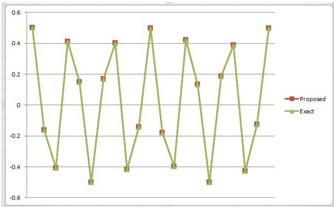 Figure 1: Approximate solutions of $\ddot{x} + \dot{x} = x \dot{x}\ddot{x}$ for $A = 0.5$ Compare with the corresponding numerical solution. 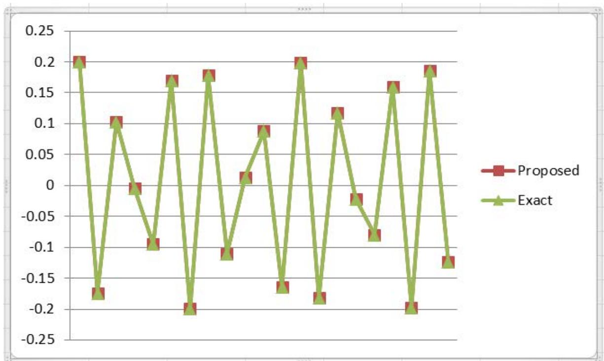 Figure 2: Approximate solutions of $\ddot{x} + \dot{x} = x\dot{x}\ddot{x}$ for $A = 0.1$ Compare with the corresponding numerical solution. ## V. CONVERGENCE AND CONSISTENCY ANALYSIS Test of convergence: The iteration method will be convergent if the set of solutions $x_{k}$ (or frequencies $\Omega_{k}$ or amplitudes $\mathrm{T_k}$ ) in ascending order satisfy the following property. $x_{E} = \operatorname{Lim}(x_{k})$ or, $\Omega_{E} = \operatorname{Lim}(\Omega_{k})$ or, $\mathrm{T}_{E} = \operatorname{Lim}(\mathrm{T}_{k})$, $k \to \infty$. Here $x_{E}$ is considered as the exact solution, $\Omega_{k}$ denotes the frequencies and $\mathrm{T}_{k}$ denotes the corresponding periods of the nonlinear oscillator. In the obtained solutions, it has been indicated that there is less error to iterative steps in ascending order and finally it has been shown that $|T_2 - T_E| < \varepsilon$, where $\varepsilon$ is a small positive number. Hence the presented extended iteration method is convergent. Test of consistency: The iterative method will be consistent if the set of solutions $x_{k}$ (or frequencies $\Omega_{k}$ or amplitudes $T_{k}$ ) in ascending order satisfy the following property $$ \operatorname {L i m} | x _ {k} - x _ {E} | = 0 \mathrm {o r}, \operatorname {L i m} | \Omega_ {k} - \Omega_ {E} | = 0 \mathrm {o r}, \operatorname {L i m} | T _ {k} - T _ {E} | = 0, k \to \infty $$ In the obtained solutions, it has been indicated that there is less error to iterative steps in ascending order, and finally, it has been shown that, $$ \operatorname {L i m} | T _ {k} - T _ {E} | = 0, k \to \infty \mathrm {a s} | T _ {2} - T _ {E} | = 0. $$ Hence the presented extended iteration method is consistent. ## VI. CONCLUSION In this research, it has been seen that the most significant part of solutions has been enhanced drastically. The modified solutions show that this modification is more precise than other existing solution methods and resolution is valid for the large amplitude of oscillation for the jerk system. We have seen that it is not always true that the extended iteration method yields better results than the direct iteration method. It can be accomplished that the adopted modification is steadfast, effectual, and conformable also, it, also present sufficient well-suited solutions to the nonlinear jerk equations arising in mathematical physics, applied mathematics, and different field of engineering, specially in Mechanical, Electrical, and Space engineering. Availability of Data This study was not supported by any data. Conflict of Interest The authors affirm that they are impartial.

Generating HTML Viewer...

References

21 Cites in Article
M Alquran,K Al-Khaled (2012). Effective approximate methods for strongly nonlinear differential equations with oscillations.
M Alquran,N Doğan (2010). Variational Iteration method for solving twoparameter singularly perturbed two point boundary value problem.
A Beléndez,A Hernández,T Beléndez,E Fernández,M Álvarez,C Neipp (2007). Application of He's Homotopy Perturbation Method to the Duffing-Harmonic Oscillator.
A Elías-Zúñiga,O Martínez-Romero,R Córdoba-Díaz (2012). Approximate solution for the Duffing-harmonic oscillator by the enhanced cubication method.
H Gottlieb (2004). Harmonic balance approach to periodic solutions of non-linear jerk equations.
B Haque (2014). A New Approach of Mickens' Extended Iteration Method for Solving Some Nonlinear Jerk Equations.
B Haque,S Flora (2020). On the analytical approximation of the quadratic non-linear oscillator by modified extended iteration method.
B Haque,M Ikramul,Hossain (2021). An analytical approach for solving the nonlinear jerk oscillator containing velocity times acceleration-squared by an extended iteration method.
M Hosen,M Chowdhury,M Ali,A Ismail (2016). A comparison study on the harmonic balance method and rational harmonic balance method for the Duffing-harmonic oscillator.
H Hu,J Tang (2006). Solution of a Duffing-harmonic oscillator by the method of harmonic balance.
H Hu,J Tang (2007). A classical iteration procedure valid for certain strongly nonlinear oscillators.
Gamal Ismail,Hanaa Abu-Zinadah (2021). Analytic approximations to non-linear third order Jerk equations via modified global error minimization method.
M Karahan,Fatih (2017). Approximate solutions for the nonlinear third-order ordinary differential equations.
Xiaoyan Ma,Liping Wei,Zhongjin Guo (2008). He's homotopy perturbation method to periodic solutions of nonlinear Jerk equations.
R Mickens (1984). Comments on the method of harmonic balance.
R Mickens (1987). Iteration procedure for determining approximate solutions to non-linear oscillator equations.
R Mickens (2010). Truly nonlinear oscillations: harmonic balance, parameter expansions, iteration, and averaging methods.
A Nayfeh (1973). Perturbation Methods, Ali Hasan Nayfeh, Chichester. John Wiley & Sons. 1973. 425 pp. £9.00..
T Ozis,A Yildirim (2007). Determination of the frequency-amplitude relation for a Duffing-harmonic oscillator by the energy balance method.
J Ramos (2010). Analytical and approximate solutions to autonomous, nonlinear, third-order ordinary differential equations.
Explore published articles in an immersive Augmented Reality environment. Our platform converts research papers into interactive 3D books, allowing readers to view and interact with content using AR and VR compatible devices.
Your published article is automatically converted into a realistic 3D book. Flip through pages and read research papers in a more engaging and interactive format.
Mathematics has applications in every aspect of real life. So many such type of real-life problems are modeled by differential equations. Therefore, differential equations are used as tools to solve many complex situations. With the help of differential equations, we can find the formula to solve many significant issues in many areas of the Anatomy and Physiology of the human body like physical, mental physical, and medical principles. Differential equations can be linear, nonlinear, autonomous, or non-autonomous. Practically, most of the differential equations involving physical phenomena are nonlinear. Hence nonlinear differential equations play a vital role in case of science and engineering. Nonlinear systems are differently classified, and the ‘nonlinear jerk oscillator’ is one of the most essential parts of a nonlinear system. Different types of nonlinear jerk oscillators will be analyzed using Extended Iteration Method, and the outcome may leave an impact to be better than the current results.
Our website is actively being updated, and changes may occur frequently. Please clear your browser cache if needed. For feedback or error reporting, please email [email protected]
Thank you for connecting with us. We will respond to you shortly.