I. INTRODUCTION

The supply of planted forests with homogeneous dimensions favors creating business rules to support wood management and processing. As a result, information reported of the pieces milled per tree or log (number, volume and potential revenue), allows suppliers the opportunity to trade their wood in more profitable markets (Costa et al. 2016).

Business rules can also assist in the native forest wood trade with some limitations, due to different ages and heterogeneous dimensions. An example is the Brazil concessions for management plans in national conservation forests, which has been making since 2014. By means of monitoring and inspection systems, the product from tree to sale is tracked, guaranteeing the legalization of logging products. An essential variable in this process is the yield of lumber, which depends on the diameter of the logs, the combination of the cutting pattern with the dimensions of the pieces, and the occurrence of defects, such as knots, tortuosity, and cracks, as well as the general health/quality of the lumber (Bonato et al. 2017; Cunha et al. 2015; Juizo et al. 2014; Mahica et al. 2013; Rocha and Tomaselli 2002).

Currently, monitoring and inspection systems use a volumetric yield coefficient of $35\mathrm{\%}$, which is the ratio between the volume of milled wood and the total log volume (Brazil 2016). When applying this coefficient, if the sawmill obtains a yield lower than this percentage, it can receive authorization to extract wood from the forest above what was established by the management plan. If the yield is higher than $35\mathrm{\%}$, the supplier must retain the surplus wood in the yard without a sales receipt.l.e. the technical criteria is not suitable, which consequently increases the environmental impact on the forest or give costs for sawmills.

Given that the volumetric performance studies used to inform the environmental agency of the actual yield of milled wood are expensive and may vary according to the demand for milled products and the quality of the wood in stock, it would be advisable to use software to perform this estimate instead of adopting a fixed, arbitrary value for several sawmills. Another function of this software would be to support production planning so that sawmills could estimate the stock and revenue of milled pieces.

Computational tools used for estimations in multiple tree products are not a novelty. Most of these tools are used to optimize wood volume for firewood, cellulose pulp and lumber (Binoti 2012; Oliveira et al. 2011; Oliveira 2011; Soares et al. 2003; Chichorro et al. 2003; Leite 1994) or estimate growth in forest production and milled wood; examples include Dyna Tree, Saw Model and Sigma E softwares (Nunes 2013; Leite 1994), Sis Eucalipto (Oliveira 2011), and RPF (Binoti 2012). There are also scanning methods (Halabe et al. 2011) that evaluate or simulate sawmill processes (Vergara et al. 2015; Murara et al. 2013; Voronin et al. 2012; Heinrich 2010; Maturana et al. 2010; Baesler et al. 2004; Lin et al. 1995; Steele 1984).

Computational solutions for lumber, which calculate the conversion into milled pieces, are intended for commercial use or were developed solely for technical and scientific purposes. Among the commercial applications are MaxiTora (Serpe et al.

2018; OpTimber 2020), CutLog (TEKL STUDIO 2018), TimberLOG (Timber Vision 2020), and Pitago Optimizers (2020). Most of these solutions are based on linear programming, a technique applied to optimize the dimensions of selected pieces in a section of the trunk.

CalcMadeira provides a new solution when simulating cut patterns applied to trees or individual logs. Its algorithms use trigonometric rules (i.e., arrow concepts, string, sine, and cosine) rather than optimization techniques (Costa et al. 2019a; 2019b; 2020).

Most sawmills do not adopt a cut pattern model. Instead, they entrust the cutting performance to the experience of the saw operator. Therefore, a pattern that parallels the empirical procedure performed by the operator is proposed. In the approximated pattern, the log is turned ${180}^{\circ }$ and ${90}^{\circ }$. The parameters used in this model are cited in the method described later in this article.

The goal of this work is to show and validate these cut models (circumscribed square, longitudinal (tangential), turn ${180}^{\circ }/{90}^{\circ }$ and the radial), comparing the accuracy between the number of pieces of wood calculated by the software and that obtained by the sawmill or by drawing in the face of the log.

II. MATERIALS AND METHODS

In this section, the models for trees and milled wood are described, followed by the structure of the tests. Then, data is collected and calculated, and the statistical analysis is presented.

a) Taper model

The software adjusts taper functions using the Kozak et al. (1969) model and volume with the

Schumacher and Hall (1933) model from taper data to estimate milled product from trees. The Smalian formula is used to estimate the milled product from log.

b) Models for milled wood

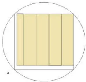
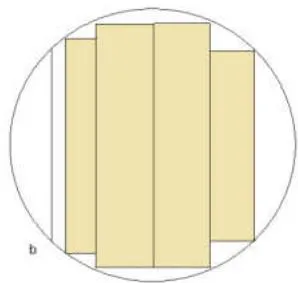
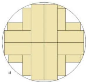
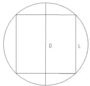
As shown in Figure 1, four slab cuts are made to the circumference for the circumscribed square cut pattern. The saw stays in the remaining square and begins to saw the lumber. In the longitudinal cut pattern, the saw first cuts the lateral slab and then begins parallel cuts on another side with the last amount of the slab cut. The model that rotates the log at 180 and 90 degrees combines the two models previously described. To begin this cut, the angle $a$ is defined for the slab (Figure 2). The chord is the width $(L)$ available for lumber and is calculated by Equations 1, 2, and 3, where $D$ is the diameter of the log, the arrow $(f)$ is a parameter that increases as the pieces are selected, and $(b)$ is the angle calculated from the thickness of the lumber.

In the model that rotates the log, when $f$ reaches the limit established by the radius ratio, which is the parameter that defines the maximum $f$ for the longitudinal cut, the cut is interrupted. The same procedure is repeated on the opposite side (i.e., a ${180}^{\circ }$ turn of the log). With the second interruption, the remainder (i.e., a rectangle plus two slabs) is rotated ${90}^{\circ }$ to perform the procedure using the circumscribed square model, where $L=\frac{D}{\sqrt{2}}$.

Fig. 1: Cut patterns for milled wood: a) circumscribed square; b) longitudinal; c) ${180}^{\circ }{90}^{\circ }$ turn log; and d) radial

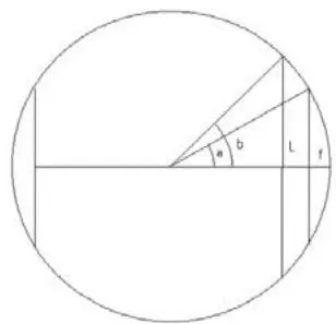
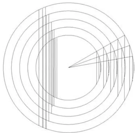
The slab is defined to find the smallest piece width. The angle generated in the cut of the slab is proportional to the diameter of the log in the milling operation. Smaller logs will have larger slab angles, while larger logs will have smaller slab angles (Figure 3). In the first version of the proposed software, the parameter "average angle of the slab" was considered. From this angle, logs with smaller diameters have an undersized initial width, which will not result in errors because the algorithm will increase the width of the slab until it reaches the width of the piece. In contrast, logs with larger diameters may experience aloss in the number of pieces, especially those of smaller widths, due to the estimation of slab areas with larger widths than those executed in the saw mill.

The distance between the radius ratio values increases with the diameter of the log; then, logs with large sections need smaller intervals between radius ratios in the simulated case (Figure 3).

One way to define the slab angle is to observe the cut of the first slab on logs with different diameters and select the grade closest to those used in the milling operation. The same procedure can be performed for the radius ratio.

Fig. 3: Slab angles of 10, 20, and ${30}^{\circ }$, which show variable slab widths (right side of the circle) and chords defined by radius ratios of 0.55, 0.60, and 0.65 (left side of the circle) concerning to logs with diameters of 20, 25, 30, 35 and 40 cm

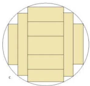
The radial cutting model (Figure 1) consists of dividing the log to quadrants and calculating sawn pieces to the radius direction. The cutting of parts is run by alternating the edges within the quadrant, limited to two slices by an angle of ${45}^{\circ }$. Calculations are performed for one quadrant and multiplied by 4 for the log.

All models were validated with draws in digital graphics using the CAD software Libre CAD (2020).

c) Data

Six tests were performed with trees and logs by applying the circumscribed square, longitudinal (tangential), ${180}^{\circ }$ and ${90}^{\circ }$ turnlog, and radial cut patterns (Table 1). These tests range from more controlled to more sampled.

Test	1	2	3	4	5	6
Cut pattern	Circumscribed square	Empiric	Longitudinal	Longitudinal	Turns of 180 and 90°	Radial
Cut model applied	Circumscribed square	Circumscribed square	Longitudinal	Longitudinal	Turns of 180 and 90°	Radial
Source	Tree	Tree	Log	Log	Log	Log
Quantity dbh/h/hc/bark%	3 trees/16 logs	3 trees/19 logs	9	19	51	6
Tree 1	24/25.2/10.7/8.7	24/25.2/10.7/8.7
Tree 2	21/22/11.3/4.8	21/22/11.3/4.8
Tree 3	19.5/24.4/11.4/8.5	19.5/24.4/11.4/8.5
Range of logs diameters (cm)	9-22	9-24	13-22	19-46	19-38	28-61
Lumber type	NBR 14807*	Clapboard 50 x 30 mm Clapboard 40 x 30 mm Board 100 x 30 mm	Clapboard 40 x 20 mm	Board 50-400 x 27 mm Large board 50-400 x 40 mm Step width 50 mm	Board 50-400 x 27 mm Large board 50-400 x 40 mm mm Step width 50 mm	Board 50-600 x 27 mm Step width 50 mm
Length (m) of log	2	3.1	3.1	3.4	3.4	1.5-2.9
Priori of lumbers	By size	User choice	User choice	None	None	None

i. Test 1

In this test, we applied the rule of priority by size in width and thickness to calculate lumber pieces of small trees of the Corymbiacitriodora species planted from seeds, which had some tortuosity in the trunk. The trees were cut and processed in a sawmill of the Embrapa company in Sete Lagoas, Minas Gerais State, Brazil.

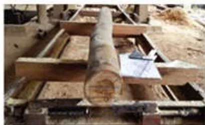
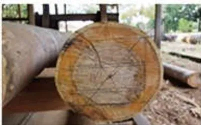
The Kozak taper model was applied to each tree. The lumber pieces calculated by the proposed software were drawn in the most minor section of each log before being sawed (Figures 4a and b). The diameters with bark (di_log) were measured, and the width of the lumber (wi_log) was framed in the log section.

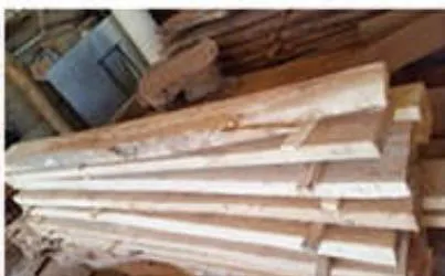
The milled pieces were measured in width (wi_sw) and thickness (th_sw) at the ends and in the middle of the lumber (Figure 4c).

A

b

C Fig. 4: a) Log in the sawmill machine, b) smaller face of a log with pieces calculated and selected to be cut, and c) stacked pieces to dry after measurement and identification

ii. Tests 2 and 3

In Test 2, It is compared results among the Calc Madeira and CutLog softwares. The trees were cut in Maravilhas city, Minas Gerais State, and transported to a sawmill in Matosinhos city, Minas Gerais.

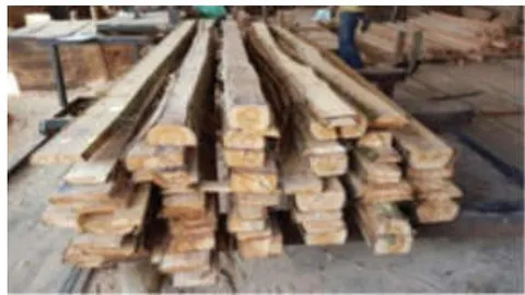
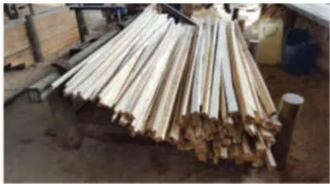
It is used nine trees close to the evaluated trees (i.e., those that were milled) for generate taper model. The width and thickness of the pieces were not measured according to uniformity in production and the constant width and thickness of the lumber. Only the number of pieces per log was obtained (Figure 5), and imperfections, such as tortuosity and cracks, were noted.

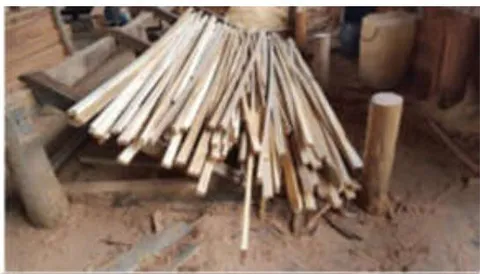
In Test 3, It is cut a new set of 3 trees of the Corymbia citriodora species. However, evaluations were performed by individual logs without the need for taper models, already validated in Test 1. As in Test 2, only the number of pieces per log was obtained (Figure 6).

a

b

b Fig. 6: a) First product of the longitudinal cut pattern and b) clapboards after the second step in a circular blade

iii. Tests 4 and 5

In Test 4, it is measured nineteen logs, and in Test 5, fifty-one logs, both from eucalyptus with different ages and genetic materials (i.e., stock). The tests were performed in a sawmill in the municipality of Martinho Campos, Minas Gerais. The pieces milled were boards larger than or equal to $50\mathrm{mm}$ in width up to the maximum width allowed by the diameter of the log. The thickness was fixed at $27\mathrm{mm}$. The $40\mathrm{mm}$ thickness was milled in the center of the log to prevent the large board from cracking in its core. The cut pattern was longitudinal for Test 4 and turns of ${180}^{\circ }$ and ${90}^{\circ }$ for Test 5. In these tests, only the width was measured.

iv. Test 6

This test was performed at the Embrapa farm in Sete Lagoas, Minas Gerais. Six logs from Pinus sp and Araucaria angustifolia trees with different displacements of the pith with reference to the center of the face of the log were measured in Test 6. The pieces were drawn in small sections of the logs. These pieces were boards larger than or equal to $50\mathrm{mm}$ in width up to the maximum width allowed by the circumference of the log's barkless wood. The drawing was performed in all quadrants with points of origin in the marrow, which resulted in quadrants of different sizes. The intention was to detect bias among the calculated pieces based on the center of the log section and the pith deviated.

The thickness was fixed at $32\mathrm{mm}$, which matches a thickness of $27\mathrm{mm}$ plus $5\mathrm{mm}$ considering the consumption of wood by the saw.

In this test, it is assessed the accuracy of the number and dimension of pieces that the program calculated to the pieces observed in the logs. Accuracy is reported per log as a function of pith displacement.

v. Sawmill operations

Tests 2, 3, 4, and 5 followed the operational procedure without drawing pieces in the logs and informing the operator of the number of pieces. With this, the sawmill chose the pieces of interest with their given dimensions and established the priority among them to mill.

The empirical method applied in Tests 2 and 5 by different operators in sawmills begins with sawing the lateral slab and sawing pieces up to a limit defined by the operator. Then, the log is rotated, which can be at ${180}^{\circ }$ or ${90}^{\circ }$ angles. This process does not precisely follow the model of the first ${180}^{\circ }$ turn, as after turning ${90}^{\circ }$. It can vary from log to log too. However, this operation reduces the log to a rectangle plus two slabs where boards are milled with the same widths. The large board is sawed in its core.

d) Calculations

The following data are used to execute the cut model algorithms: dimensions of the lumber, including length, width, and thickness; and measurements of the tree, including dbh, total and commercial height, and bark thickness measured at each section of the log, being considered the average per tree.

In individual log algorithms, the parameters are smaller diameter, larger diameter, and log length. The wood loss established by the saw thickness was $5\mathrm{mm}$, a parameter informed of the application according to the saw type.

In Tests 3 and 4 for the longitudinal model, the slab lateral angle was ${30}^{\circ }$. In Test 5, three medium angles for the lateral slab $({10}^{\circ },{20}^{\circ },$ and ${30}^{\circ })$ and three radius proportions (0.55, 0.60, and 0.65) were chosen after monitoring the process of the empirical milling technique.

e) Statistical Analysis

The statistical comparison varied with the tests because they were adapted to sawmill procedures and the characteristic of the application. The main comparison between the results obtained in the sawmill and calculated by the software was the standard error:

In Test 5, the range of the width and quantity of pieces allowed us to arrange data in the frequency distribution. The nonparametric statistics with 0.05 significance were applied to normality tests (i.e., the Shapiro-Wilk test), calculated, and then the observed data were compared using the Chi-square test and the correlation test. Spearman's correlation was applied to errors in the number and volume of pieces to verify their dependency with the diameter of the log. To do this, the differences were converted in a module for the rank of posts to assess only the magnitude of the error as a function of the log diameter. The tendency was evaluated graphically.

In Test 6, a comparison test (i.e., the Kolmogorov-Smirnov test) was performed between the calculated and observed widths of each piece. The SE% was obtained between the observed and the calculated width.

III. RESULTS AND DISCUSSION

a) Test 1

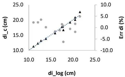
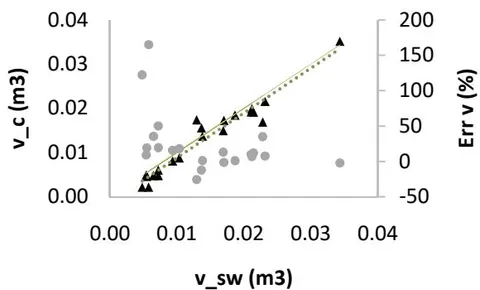
From the taper Kozak equations of trees 1, 2, and 3, the $R^2$ values were 98.2, 98.6, and $99.3\mathrm{\%}$, respectively. Figure 7 shows the agreement between values estimated by the taper equation and those measured on the log. The errors were less than $10\mathrm{\%}$ for the diameter with bark (di_log) and less than $15\mathrm{\%}$ for log volume (vr).

Fig 1

Fig. 7: a) Scattering between the observed diameter withbark (di_log) and the calculated diameter with bark (di_c) and its accuracy (Err di), and; b) scattering between the log volume (vr_log) and the calculated log volume (vr_c) and its accuracy (Err vr) For the milled pieces, Figure 8a shows the piece width $(wi\mathrm{\_}c)$ and the milled piece width $(wi\mathrm{\_}sw)$. The comparisons between thickness $(th\mathrm{\_}c)$ and thickness measured in the milled pieces $(th\mathrm{\_}sw)$ are represented in Figure 8b. The more significant divergence in the thickness of the samples was due to an uncontrolled factor in the saw operation caused by fluctuation of the log on the mill track during its course. More advanced machinery would increase the accuracy between the programmed and sawed thicknesses. This tendency was more significant in widths with underestimating of the milled piece volume (Figure 8a).

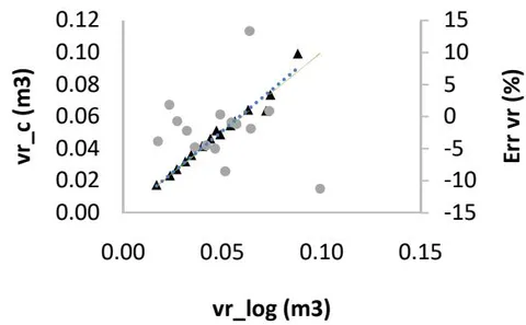
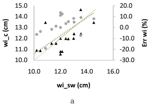
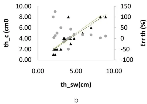
the footnote of Table 2, which shows the accuracy between the number of calculated and milled pieces).

Id0	Piece	n_c	n_sw	n_er
11	Board	3	3	0
12	Board	2	2	0
12	Board	1	1	0
13	Board	2	2	0
13	Board	1	1	0
14	Board	2	2	0
14	Board	1	1	0
15	Board	2	2	0
15	Board	1	1	0
211	Board	3	-
22	Board	2	2	0
22	Board	1	1	0
23	Board	2	2	0

Id0	Piece	n_c	n_sw	n_er
232	Board	1		-1
24	Beam	1	1	0
253	Beam	1		-1
31	Board	2	2	0
31	Board	1	1	0
32	Board	2	2	0
32	Board	1	1	0
334	Beam	1	2	1
34	Beam	1	1	0
35	Rafter	1	1	0
36	Rafter	1	1	0
Total		33	32	-1

Id0	Piece	n_c	n_sw	n_er
232	Board	1		-1
24	Beam	1	1	0
253	Beam	1		-1
31	Board	2	2	0
31	Board	1	1	0
32	Board	2	2	0
32	Board	1	1	0
334	Beam	1	2	1
34	Beam	1	1	0
35	Rafter	1	1	0
36	Rafter	1	1	0
Total		33	32	-1

• Tree and Log.
• It was impossible to mill because the length was less than the minimum limit for the mill (2 meters).
• 2 It was impossible to mill the last piece: one calculated board.
• 3 It was impossible to mill because of the log tortuosity.
• 4 The calculation indicated a beam, but two boards were milled.

b) Test 2

The taper Kozak equation from nine trees in Test 2 yielded an $R^2=99\mathrm{\%}$. There were fourteen results with biased results above $10\mathrm{\%}$ in 19 data (Figure 10a). The accuracy for the diameter with bark ( $d_i$ ), although with few results above $10\mathrm{\%}$, showed more significant inaccuracy than Test 1. The consistency was affected by the tendency (Figures 10a and b), and the expected overestimate of the milled piece number and volume.

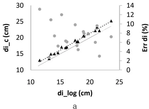
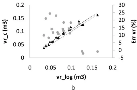
Table 3 shows the results of the sawmill and those calculated by the software. At the sawed pieces, it was not possible to obtain boards, which are the third priority (Table 1). Milling into broad pieces to get large clapboards (priority pieces with a smaller width than the board) renders it impossible to see board widths from leftovers. The calculated results showed this condition.

The CalcMadeira software calculated one hundred and four large clapboards and fifteen clapboards, with a volume of $0.5208{\text{m}}^3$ and a yield of $31\mathrm{\%}$. The data observed in the sawing procedure were one hundred and six big clapboards and thirty-two clapboards, with a volume of $0.5723{\mathrm{m}}^3$ and a yield of $37\mathrm{\%}$. An empirical method that comes close to the block was used, and the operator skill increased the yield sawing clapboards (i.e., smaller pieces) in the slabs.

The CutLog optimization module Cut Pattern Optimizing Function, which considers a priority region (middle boards) and a secondary one (sideboards), calculated the quantity of pieces close to the result of milled pieces, diverging in eight clapboards and four large clapboard pieces. This algorithm, in the secondary area of the log, advances to the slab area to obtain smaller pieces.

	Large clapboard	Clapboard	Board	Total	Volume (m3)	Yield (%)
Sawmill*	106	32	-	138	0.572	37
CalcMadeira	104	15	-	119	0.521	31
CutLog	110	40	-	150	0.591	38

c) Test 3

The number of pieces, which is shown by log, are provided in Table 4. The most significant difference occurred in Log 2, where six fewer amounts were calculated than the number of pieces milled. In total, ninety-one clapboards were calculated with a volume of $0.2257{\text{m}}^3$ and a yield of $30.1\mathrm{\%}$. The results obtained in the milled wood were ninety-three clapboards, with an output of $30.4\mathrm{\%}$.

Log	n_c	n_sw	n_er
1	20	17	3
2	13	19	-6
3	10	7	3
4	10	12	-2
5	9	9	0
			Total

d) Test 4

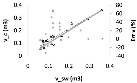
The nineteen sampled logs had a total volume of $4.837{\text{m}}^3$, and the milled volume was $2.5137{\text{m}}^3$ in sawed lumber. There is a significant variation in shape, with logs close to the cylindrical shape, except for one log with $2.65\text{cm/m}$. The taper was $0.80\text{cm/m}$, and the final yield was $58\mathrm{\%}$.

The total calculated volume was $2.7971{\mathrm{m}}^3$, with a bias of $11.3\mathrm{\%}$, and approximately $53\mathrm{\%}$ of the results per log had an error above $20\mathrm{\%}$. Figure 11 shows the bias results with the overestimating of the volume milled per log.

e) Test 5

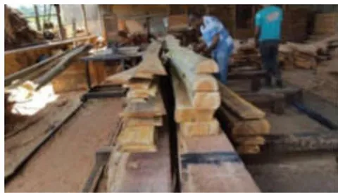
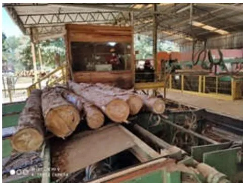
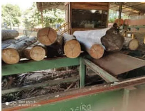
The fifty-one sampled logs had a total volume of $10.943{\mathrm{m}}^3$ and a milled volume of $6.149{\mathrm{m}}^3$ in sawed lumber. There is a significant variation in shape, with logs close to the cylindrical shape and others with more than $2\mathrm{cm}/\mathrm{m}$. The same is valid for yields, ranging from 24 to $72\mathrm{\%}$. The average taper was $0.95\mathrm{cm}/\mathrm{m}$, and the final yield was $56\mathrm{\%}$. Figure 12 shows a set of logs sent to the saw. The $42\mathrm{cm}$ diameter log (more extensive) had an irregular base, and the $27\mathrm{cm}$ log had protuberances of branches, showing the heterogeneity of the sampled material. High yields, near $70\mathrm{\%}$, may be related to the operator skill when rotating the log and the specification, which allows small pieces, such as boards from $50\mathrm{mm}$ in width.

i. Calculated and milled pieces

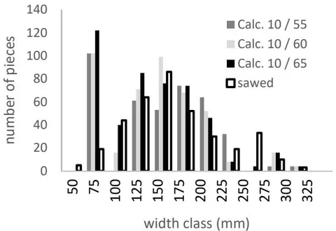
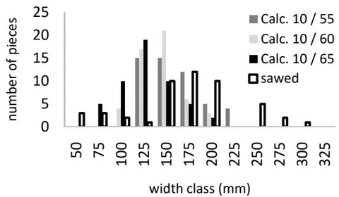
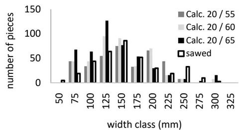
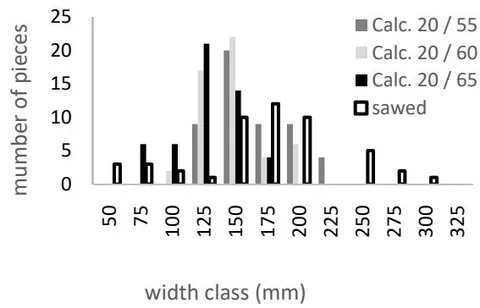
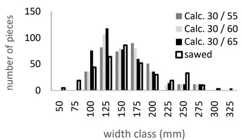
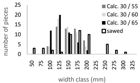
Figure 13 shows the distribution of the number of (a) boards and (b) large boards milled and calculated by width classes in $25\mathrm{mm}$ increments, according to the average angle of the slab and the proportion of the radius. The frequency of distribution in the number of pieces calculated and the number of pieces milled did not significant by the Shapiro-Wilk test (Table 5). The frequency of the calculated boards is high in the first class of widths and approaches the expected frequency with an increase in the slab angle.

The Chi-square test for comparing the observed and expected distributions of milled pieces, as shown in Table 5, shows inequality (nonadherence) between the distributions of milled and calculated boards and large boards. Although there is inequality between the distributions assessed from a critical level of probability, an inference is possible by analyzing the magnitude of the Chi-square values. Regardless of the radius proportion, the distribution of the calculated boards at ${30}^{\circ }$ for the slab was closer to that of the milled boards.

Large boards in the central part (i.e., the rectangle with two slabs) show a worse approximation between the milled and calculated distributions (Figure 13b and Table 7).

A slightly better approximation was achieved for combining the parameters (i.e., the slab angle and radius ratio) between the frequency distributions for the board with as lab angle of ${30}^{\circ }$ and a radius ratio between 0.55 and 0.60. To large board, a suboptimal approximation occurred for the frequency distribution with angle of ${20}^{\circ }$ and a radius ratio of 0.55.

Test	Ang.	Board			Milled		Large board		Milled
		0.55	0.60	0.65	0.55	0.60	0.65
S-W	10	0.130	0.160	0.226	0.031	0.056	0.162
C-S	10	518.1	452.5	625.4	217.0	292.0	378.8
S-W	20	0.121	0.129	0.186	0.019	0.043	0.131
C-S	20	157.8	150.5	282.8	90.9	291.3	438.9
S-W	30	0.044	0.052	0.077	0.054	0.061	0.104
C-S	30	110.4	90.7	114.1	186.9	310.3	434.5
S-W					0.098				0.036

a b Fig. 13: Frequency of a) boards and b) large boards milled and calculated by width class with $25\mathrm{mm}$ increments, and an average angle of the slab of ${10}^{\circ }$, ${20}^{\circ }$ and ${30}^{\circ }$

In evaluating errors between the calculated and milled pieces according to the diameter of the log and the occurrence of trends (Table 6), there were two positive correlations for the number of pieces and five negative correlations for the volume of pieces with a significance level of 0.05.

Based on the significance and the signal and magnitude of the correlations, these results did not indicate that the error in the number of pieces will increase with the diameter of the log. However, they did suggest a tendency to reduce the error in the volume of pieces in logs with larger diameters.

Ang.	0.55	n err 0.60	0.65	0.55	err v (%)
					0.60	0.65
10	0.211	0.355 *	0.041	-0.292 *	-0.280 *	-0.216
20	0.053	0.257	0.331 *	-0.233	-0.210	-0.249
30	0.020	0.087	0.242	-0.362 *	-0.389 *	-0.434 *

Figure 14 shows the scattering between the observed and estimated piece volumes per log for slab angles of 10, 20 and ${30}^{\circ }$, and varying radius ratios of

0.55, 0.60 and 0.65. The lowest deviations occurred for the ${30}^{\circ }$ angle, regardless the radius proportions.

a

b C Fig. 14: Scattering between the volume of calculated and milled pieces per log for slab angles of a) ${10}^{\circ }$, b) ${20}^{\circ }$, and c) ${30}^{\circ }$

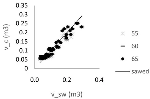
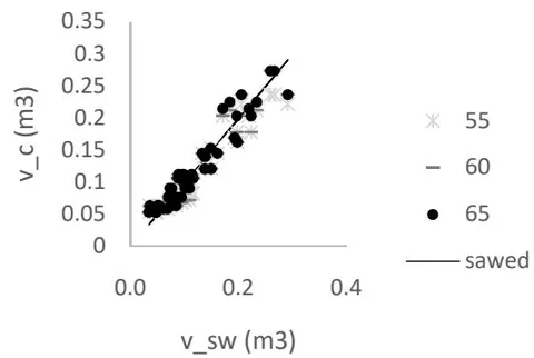
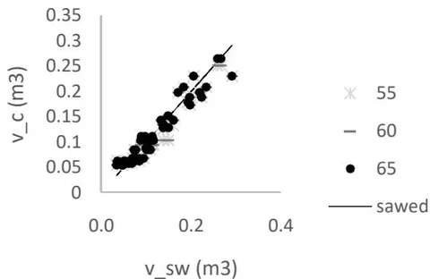
Table 7 shows the totals calculated and the accuracy about the total number of milled pieces. The accuracy varied from -1.4 to $27.1\mathrm{\%}$ for the number of pieces and from -7.6 to $-0.7\mathrm{\%}$ for the volume of pieces. Overestimates are noted for the number of pieces and underestimates for the volume of pieces, showing an optimal combination between the angle defined for the slab and the limit to the longitudinal cut by the proportion of the radius. The errors in the number and volume of pieces are inversely proportional.

For the total number of pieces, the best combination in terms of accuracy was the ${20}^{\circ }$ slab angle and 0.55 radius ratio. For total volume, the best accuracy was obtained using the ${20}^{\circ }$ angle and 0.65 radius ratio; It was achieved an accuracy of $0.7\mathrm{\%}$. It was obtained the best combination of total values using the ${30}^{\circ }$ angle for the slab with a radius ratio of 0.60; accuracies of 2.2 and $-5.4\mathrm{\%}$, respectively, were obtained. The estimated yield was $53\mathrm{\%}$ yield, and the actual yield obtained at the sawmill was $56\mathrm{\%}$.

	n			v			Yield
	0.55	0.60	0.65	0.55	0.60	0.65	0.55	0.60	0.65
10	445	487	526	5.71	5.94	6.04	0.52	0.54	0.55
20	410	461	515	5.68	5.97	6.19	0.52	0.55	0.57
30	408	423	461	5.76	5.82	5.97	0.53	0.53	0.55
Milled		414		Error%	6.15			0.56
10	7.5	17.6	27.1	-7.1	-3.4	-1.7
20	-1.0	11.4	24.4	-7.6	-2.9	0.7
30	-1.4	2.2	11.4	-6.3	-5.4	-2.8
Total Vr					10.94

Note: Large boards and boards were added because one large board is calculated per log; that is, the constant value of the fifty-one large boards. In the milled material, forty-nine large boards were obtained; that is, it was not possible to extract two boards.

f) Test 6

Figure 15 shows designed pieces in a small section of the logs with a source on marrow.

1

2

3

4

5

6 Fig. 15: Designed sections of Logs 1-6 with pieces of thickness $32\text{mm}$ ( $27+5\text{mm}$ ) and width and marrow bias of $2\text{cm}$ ( $\log 1$ ); $4\text{cm}$ ( $\log 2$ ); $4.5\text{cm}$ ( $\log 3$ ); $5.3\text{cm}$ ( $\log 4$ ); $6\text{cm}$ ( $\log 5$ ) and $6.5\text{cm}$ ( $\log 6$ )

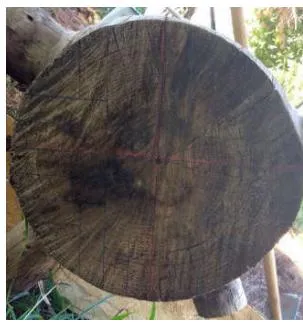
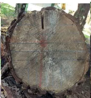
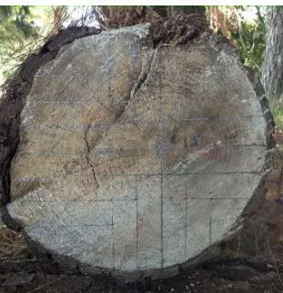
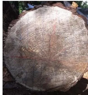
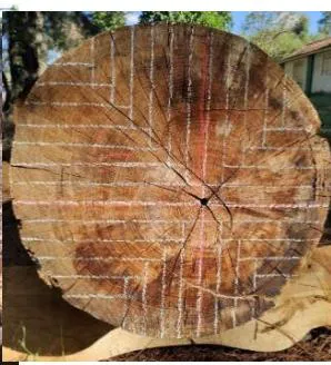
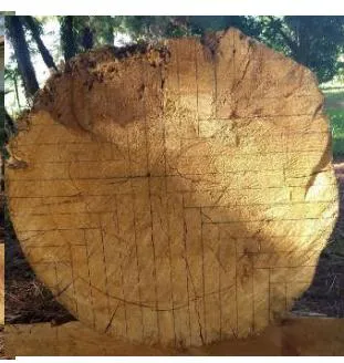
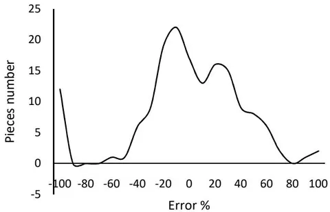
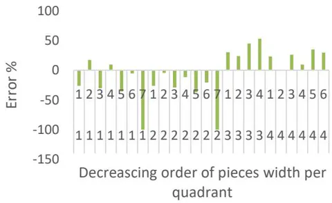
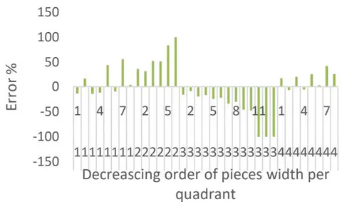
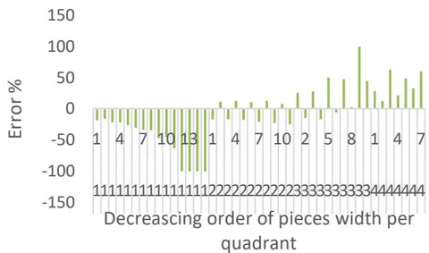
Figure 16 shows that a perceptual error of width between -30 and 30 represents $65\mathrm{\%}$ of the pieces. The software did not calculate 12 pieces $(-100\mathrm{\%})$ when it was possible to draw the piece. because the radial model calculates the pieces from the circumference center. However, the logs used in this work have marrow bias (Figure 15).

Fig. 16: Perceptual error frequencies in classes of $10\mathrm{\%}$

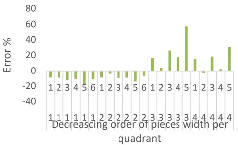
As the bias of marrow increases, the positive and negative errors will be more significant due to the quadrant differences among sources in marrow and sources in the circumference center. Figure 17 shows the error frequencies of the largest to smallest width per quadrant in each log. In the Log 1 it is possible to view the effect of the difference among center and marrow position. The drawn piece width was larger than the calculated pieces in quadrants 1 and 2, inverting the error in quadrants 3 and 4. The section of this log has the smallest marrow bias, which was $2\mathrm{cm}$ (Figure 15).

1

2

3

4

5

6 Fig. 17: Errors% in decreasing order of piece width per quadrant per log (for Logs 1-6)

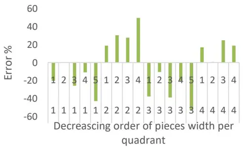
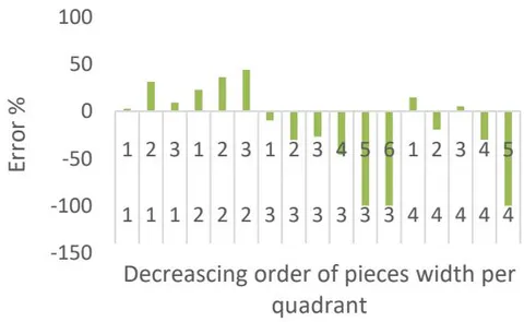
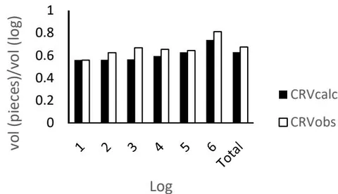
The difference between the yield coefficients (i.e., sawed volume/log volume) of the observed and calculated piece volumes was not significant than $11\mathrm{\%}$ (Figure 18). The bias of the marrow did not cause significant differences between the calculated and observed yields.

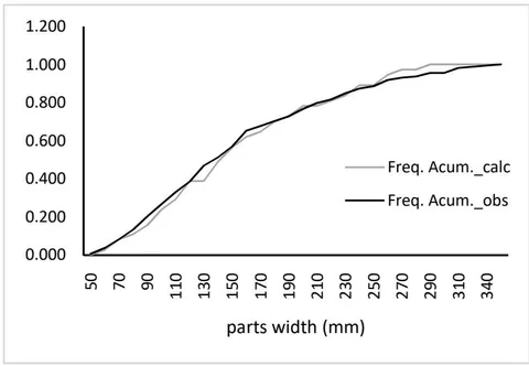
It was applied the Kolmogorov-Smirnov test to compare two samples, the calculated and observed widths. The data were grouped into observed and calculated width classes by $10\mathrm{mm}$ increments, and the cumulative frequencies of the calculated and observed widths were calculated. The total calculated pieces were 147, and the observed pieces were 158.

The larger value of K-S was 0.0806, which was smaller than the table value for the size of 30 samples and a significance level of $5\mathrm{\%}$, considering statistically equal samples (drawing in log and calculated by the software) (Figure 19).

It is usual to estimate the shape of trees using equations that include data from many trees. As a result, these equations can be applied to other trees with similar shape characteristics. However, the data per tree should be used to obtain the best shape estimate for a specific tree, even with little data. Test 1 shows the best accuracy for log dimensions when the log equation is used. The loss of accuracy for the log dimension in Test 2 was due to using an equation that was not specific to the tree.

Another insight is that other applications, such as CutLog, can have good results for the empiric procedure in the sawmill (Murara et al. 2013; Anjos and Fontes, 2017), but it works on logs individually. However, the new software used for this work processes many logs or trees at once. When the cut pattern was the same as the cut model applied, good overall results were achieved, as seen from Tests 1, 3, and 4.

The model that rotates ${180}^{\circ }/{90}^{\circ }$ the log obtained reasonable accuracy in the production of milled pieces by log, although the sawing operation performed at the sawmill is empirical, as seen in Tests 2 and 5. This operation does not precisely follow a cut pattern with pre-established parameters. It was observed that this model required a small simulation between the angle of the slab and the radius ratio to achieve closer operation parameters.

The parameters change the values according to the log size. Thus, the better approximation of the average of these values assigned in the software with the average of the radius proportions and the angles of the slab conducted by the operator, the greater the accuracy between the quantity and volume of pieces.

The calculation with trigonometric operations is accurate for obtaining pieces in a circle. The errors are related to the variations in the angles of the slab, the radius ratio that limits the cut to rotate the log and restart the cut, defects of the wood in the process (i.e., cracks or hollow wood), incorrectly defining the parameter of consumption of wood by the saws, and the difference between the theoretical cut model and that executed at the sawmill. In the case of the radial model, more significant errors are related to the bias of the marrow.

These results indicate that the application of this software can be an alternative to relationships between forest management and legal commerce of lumber products, as well as being a management tool to obtain sawmill revenue forecasts.

IV. CONCLUSION

The circumscribed square model is accurate in the control test with a taper model per tree. Still, when applied to compare with empiric procedures of sawmills, it results in an underestimate of the lumber, mainly in small pieces.

The longitudinal model had a reasonable accuracy in cut patterns with slight discrepancies.

The model of turning the log 180 and 90 degrees, combining two cut patterns, i.e., the longitudinal and circumscribed square, obtained good accuracy for some of the combinations between the angle of the slab and radius ratio when estimating the empirical milling procedure. To get the best results, observation during the milling operation is required to monitor both parameters in a heterogeneous sample of logs.

Better results of the radial model are obtained in trees with a negligible bias of the marrow relationship at the center of the circumference.

ACKNOWLEDGMENTS

This research was funded by the EMBRAPA project Sis Cerrado - Timber productivity in SIs and in reference systems of long-term physical models; SIG Solutções Ltda. Partnership; and Project N° 20.18.03.015.00.00 ILPF strategy for agricultural innovation in the Cerrado Mineiro region and bordering areas - Sis Gerais. We would like to acknowledge to saw mills S&D Madeiras and Turmalina Ltda Company for support with validation tests.