
Derivatives Pricing in Non-Arbitrage Market

§ National Academy of Sciences of Ukraine

Send Message

To: Author

Derivatives Pricing in Non-Arbitrage Market

Article Fingerprint

ReserarchID

SFR7RYFP

Derivatives Pricing in Non-Arbitrage Market Banner

Key Research Insights

Synthesized scholarly intelligence & interactive research assistant
  • English
  • Afrikaans
  • Albanian
  • Amharic
  • Arabic
  • Armenian
  • Azerbaijani
  • Basque
  • Belarusian
  • Bengali
  • Bosnian
  • Bulgarian
  • Catalan
  • Cebuano
  • Chichewa
  • Chinese (Simplified)
  • Chinese (Traditional)
  • Corsican
  • Croatian
  • Czech
  • Danish
  • Dutch
  • Esperanto
  • Estonian
  • Filipino
  • Finnish
  • French
  • Frisian
  • Galician
  • Georgian
  • German
  • Greek
  • Gujarati
  • Haitian Creole
  • Hausa
  • Hawaiian
  • Hebrew
  • Hindi
  • Hmong
  • Hungarian
  • Icelandic
  • Igbo
  • Indonesian
  • Irish
  • Italian
  • Japanese
  • Javanese
  • Kannada
  • Kazakh
  • Khmer
  • Korean
  • Kurdish (Kurmanji)
  • Kyrgyz
  • Lao
  • Latin
  • Latvian
  • Lithuanian
  • Luxembourgish
  • Macedonian
  • Malagasy
  • Malay
  • Malayalam
  • Maltese
  • Maori
  • Marathi
  • Mongolian
  • Myanmar (Burmese)
  • Nepali
  • Norwegian
  • Pashto
  • Persian
  • Polish
  • Portuguese
  • Punjabi
  • Romanian
  • Russian
  • Samoan
  • Scots Gaelic
  • Serbian
  • Sesotho
  • Shona
  • Sindhi
  • Sinhala
  • Slovak
  • Slovenian
  • Somali
  • Spanish
  • Sundanese
  • Swahili
  • Swedish
  • Tajik
  • Tamil
  • Telugu
  • Thai
  • Turkish
  • Ukrainian
  • Urdu
  • Uzbek
  • Vietnamese
  • Welsh
  • Xhosa
  • Yiddish
  • Yoruba
  • Zulu
Reading Preferences
Font Size
Line Spacing
Background
This converted HTML version may contain rendering inconsistencies. Please refer to the PDF for the authoritative version, or click here to provide feedback.

Abstract

The general method is proposed for constructing a family of martingale measures for a wide class of evolution of risky assets. The sufficient conditions are formulated for the evolution of risky assets under which the family of equivalent martingale measures to the original measure is a non-empty set. The set of martingale measures is constructed from a set of strictly nonnegative random variables, satisfying certain conditions. The inequalities are obtained for the non-negative random variables satisfying certain conditions. Using these inequalities, a new simple proof of optional decomposition theorem for the nonnegative super-martingale is proposed. The family of spot measures is introduced and the representation is found for them. The conditions are found under which each martingale measure is an integral over the set of spot measures. On the basis of nonlinear processes such as ARCH and GARCH, the parametric family of random processes is introduced for which the interval of non-arbitrage prices are found. The formula is obtained for the fair price of the contract with option of European type for the considered parametric processes. The parameters of the introduced random processes are estimated and the estimate is found at which the fair price of contract with option is the least.

I. INTRODUCTION

The study of non-arbitrage markets was begun for the first time in Bachelier's work [1]. Then, in the famous works of Black F. and Scholes M. [2] and Merton R. S. [3] the formula was found for the fair price of the standard call option of European type. The absence of arbitrage in the financial market has a very transparent economic sense, since it can be considered reasonably arranged. The concept of non arbitrage in financial market is associated with the fact that one cannot earn money without risking, that is, to make money you need to invest in risky or risk-free assets. The exact mathematical substantiation of the concept of non arbitrage was first made in the papers [4], [5] for the finite probability space and in the general case in the paper [6]. In the continuous time evolution of risky asset, the proof of absent of arbitrage possibility see in [7]. The value of the established Theorems is that they make it possible to value assets. They got a special name "The First and The Second Fundamental Asset Pricing Theorems." Generalizations of these Theorems are contained in papers [8], [9], [10].

If the martingale measure is not the only one for a given evolution of a risky asset, then a rather difficult problem of describing all martingale measures arises in order to evaluate, for example, derivatives.

Assessment of risk in various systems was begun in papers [11], [12], [13], [14].

Statistical studies of the time series of the logarithm of the price ratio of risky assets contain heavy tails in distributions with strong elongation in the central region. The temporal behavior of these quantities exhibits the property of clustering and a strong dependence on the past. All this should be taken into account when building models for the evolution of risky assets.

In this paper, we generalize the results of the papers [15], [16], [17] and construct the evolution of risky assets for which we completely describe the set of equivalent martingale measures.

The aim of this study is to describe the family of martingale measures for a wide class of risky asset evolutions. The paper proposes the general concept for constructing the family of martingale measures equivalent to a given measure for a wide class of evolutions of risky assets. In particular, it also contains the description

First, we show an integral inequality for a nonnegative random variable under the inequality for this nonnegative random variable with respect to the constructed family of measures. Further, using this integral inequality for the non-negative random variable, a pointwise system of inequalities is obtained for this non-negative random variable for a particular case. After that, the pointwise system of inequalities is obtained for the non-negative random variable in the general case. Then, using the resulting pointwise system of inequalities, an inequality is established for this non-negative random variable whose right-hand side is such that its conditional mathematical expectation is equal to one.

On the basis of the results of Section 4, in Section 5, we prove the optional decomposition for the non negative super-martingales. In Section 6, we introduce the spot measures by the recurrent relations and find the representation for them. Using these facts under certain conditions we prove integral representation for every martingale measure over the set of spot measures.

First, the optional decomposition for diffusion processes super-martingale was opened by El Karoui N. and Quenez M. C. [21]. After that, Kramkov D. O. and Follmer H. [22], [23] proved the optional decomposition for the nonnegative bounded super-martingales. Folmer H. and Kabanov Yu. M. [24], [25] proved analogous result for an arbitrary super-martingale. Recently, Bouchard B. and Nutz M. [26] considered a class of discrete models and proved the necessary and sufficient conditions for the validity of the optional decomposition.

Section 7 contains applications of the results obtained. A class of random processes is considered, which contains well-known processes of the type ARCH and GARCH ones. Two types of random processes are considered, those for which the price of an asset cannot go down to zero and those for which the price can go down to zero during the period under consideration. The first class of processes describes the evolution of well-managed assets. We will call these assets relatively stable. For the evolution of relatively stable assets in the period under consideration, the family of martingale measures is one and the same. The family of martingale measures for the evolution of risky assets whose price can drop to zero is contained in the family of martingale measures for the evolution of relatively stable assets. Each of the martingale measures for the considered class of evolutions is an integral over the set of spot martingale measures.

The interval of non-arbitrage prices is found for a wide class of payoff functions in the case when evolution describes relatively unstable assets. This range is quite wide for the payoff functions of standard put and call options. The fair price of the super hedge is in this case the starting price of the underlying asset. The estimates are found for the fair price of the super-hedge for the introduced class of evolutions with respect to stable assets. The formulas are found for the fair price of contracts with call and put options for the evolution of assets described by parametric processes.

The same formulas are found for Asian-type put and call options. A characteristic feature of these estimates is that for the evolution of relatively stable assets the fair price of the super hedge is less than the price of the underlying asset.

In Section 8, the estimates of the parameters of risky assets included in the evolution are obtained. The formulas are found for the fair price of contracts with call and put options for the obtained parameter estimates, and the interval of non-

Let {ΩN,FN,PN} be a direct product of the probability spaces {Ωi0,Fi0,Pi0}, i=1,N―, ΩN=∏i=1NΩi0, PN=∏i=1NPi0, FN=∏i=1NFi0, where the σ -algebra FN is a minimal σ -algebra, generated by the sets ∏i=1NGi, Gi∈Fi0. On the measurable space {ΩN,FN}, under the filtration Fn, n=1,N―, we understand the minimal σ -algebra generated by the sets ∏i=1NGi, Gi∈Fi0, where Gi=Ωi0 for i>n. We also introduce the probability spaces {Ωn,Fn,Pn}, n=1,N―, where Ωn=∏i=1nΩi0, Fn=∏i=1nFi0, Pn=∏i=1nPi0. There is a one-to-one correspondence between the sets of the σ -algebra Fn, belonging to the introduced filtration, and the sets of the σ -algebra Fn=∏i=1nFi0 of the measurable space {Ωn,Fn}, n=1,N―. Therefore, we don't introduce new denotation for the σ -algebra Fn of the measurable space {Ωn,Fn}, since it always will be clear the difference between the above introduced σ -algebra Fn of filtration on the measurable space {ΩN,FN} and the σ -algebra Fn of the measurable space {Ωn,Fn}, n=1,N―.

We assume that the evolution of risky asset {Sn}n=0N, given on the probability space {ΩN,FN,PN}, is consistent with the filtration Fn, that is, Sn is a Fn -measurable. Due to the above one-to-one correspondence between the sets of the σ -algebra Fn, belonging to the introduced filtration, and the sets of the σ -algebra Fn of the measurable space {Ωn,Fn},n=1,N―, we give the evolution of risky assets in the form {Sn(ω1,…,ωn)}n=0N, where Sn(ω1,…,ωn) is an Fn -measurable random variable, given on the measurable space {Ωn,Fn}. It is evident that such evolution is consistent with the filtration Fn on the measurable space {ΩN,FN,PN}.

Further, we assume that

Pn((ω1,…,ωn)∈Ωn,ΔSn>0)>0,
(1)Pn((ω1,…,ωn)∈Ωn,ΔSn<0)>0,n=1,N―,

where ΔSn=Sn(ω1,…,ωn)−Sn−1(ω1,…,ωn−1),n=1,N―.

(2)Ωn−={(ω1,…,ωn)∈Ωn,ΔSn≤0},Ωn+={(ω1,…,ωn)∈Ωn,ΔSn>0},
(3)ΔSn−=−ΔSnχΩn−(ω1,…,ωn),ΔSn+=ΔSnχΩn+(ω1,…,ωn),
Vn(ω1,…,ωn−1,ωn1,ωn2)=ΔSn−(ω1,…,ωn−1,ωn1)+ΔSn+(ω1,…,ωn−1,ωn2),
Ωn−1=⋃k=1NnVn−1k,An0,k−,An0,k+∈Fn0,An0,k−∪An0,k+=Ωn0,
(6)An0,k−∩An0,k+=∅,Vn−1k∩Vn−1j=∅,k≠j,Vn−1k∈Fn−1.

The number Nn may be finite or infinite. Since Ωn−∪Ωn+=Ωn, Ωn−∩Ωn+=∅, and Pn(Ωn−)>0, Pn(Ωn+)>0, we have

Pn(Ωn−)=∑k=1NnPn0(An0,k−)Pn−1(Vn−1k),
(7)Pn(Ωn+)=∑k=1NnPn0(An0,k+)Pn−1(Vn−1k),Pn0(An0,k−)+Pn0(An0,k+)=1.

Further, in this paper, we assume that Pn0(An0,k−)>0, Pn0(An0,k+)>0, n=1,N―, k=1,Nn―. We also assume some technical suppositions: there exist subsets Bn,i0,k−∈Fn0, i=1,In―, In>1, and Bn,s0,k+∈Fn0, s=1,Sn―, Sn>1, satisfying the conditions

Bn,i0,k−∩Bn,j0,k−=∅,i≠j,Bn,s0,k+∩Bn,l0,k+=∅,s≠l,k=1,Nn―,
Pn0(Bn,i0,k−)>0,i=1,In―,Pn0(Bn,s0,k+)>0,s=1,Sn―,k=1,Nn―,
(8)An0,k−=⋃i=1InBn,i0,k−,An0,k+=⋃s=1SnBn,s0,k+,k=1,Nn―.

Below, we give the examples of evolutions {Sn(ω1,…,ωn)}n=1N for which the representations (5) are true.

Suppose that the random values ai(ω1,…,ωi), ηi(ωi) satisfy the inequalities 0<ai(ω1,…,ωi)≤1, 1+ηi(ωi)≥0, Pi0(ηi(ωi)<0)>0, Pi0(ηi(ωi)>0)>0, i=1,N―. If Sn(ω1,…,ωn) is given by the formula

(9)Sn(ω1,…,ωn)=S0∏i=1n(1+ai(ω1,…,ωi)ηi(ωi)),n=1,N―,
S0∏i=1n(1+∑k=1Niηik(ωi)χVi−1k(ω1,…,ωi−1)aik(ω1,…,ωi)),n=1,N―,

where the random values aik(ω1,…,ωi), ηik(ωi) satisfy the inequalities

0<aik(ω1,…,ωi)≤1,1+ηik(ωi)≥0,Pi0(ηik(ωi)<0)>0,Pi0(ηik(ωi)>0)>0,

i=1,N―, k=1,Nn―, and ⋃k=1NiVi−1k=Ωi−1, Vi−1k∩Vi−1s=∅, k≠s. Then, if to put

{ωi∈Ωi0,ηik(ωi)≤0}=Ai0,k−,{ωi∈Ωi0,ηik(ωi)>0}=Ai0,k+,

we obtain

(12)Ωi−=⋃k=1Ni[Ai0,k−×Vi−1k],Ωi+=⋃k=1Ni[Ai0,k+×Vi−1k],i=1,N―.
ΔSn(ω1,…,ωn−1,ωn)≤0,(ω1,…,ωn−1,ωn)∈Ωn−,n=1,N―,
(13)ΔSn(ω1,…,ωn−1,ωn)>0,(ω1,…,ωn−1,ωn)∈Ωn+,n=1,N―.

III. CONSTRUCTION OF THE SET OF MARTINGALE MEASURES

In this section, we present the construction of the set of measures on the basis of evolution of risky assets given by the formulas (9), (11) on the measurable space {ΩN,FN}. For this purpose, we use the set of nonnegative random values αn({ω11,…,ωn−11,ωn1};{ω12,…,ωn−12,ωn2}), given on the probability space {Ωn−×Ωn+,Fn−×Fn+,Pn−×Pn+}, n=1,N―, where Fn−=Fn∩Ωn−, Fn+=Fn∩Ωn+. The measure Pn− is a contraction of the measure Pn on the σ -algebra Fn− and the measure Pn+ is a contraction of the measure Pn on the σ -algebra Fn+. After that, we prove that this set of measures, defined the above set of random values, is equivalent to the measure PN. At last, Theorem 1 gives the sufficient conditions under that the constructed set of measures is a set of martingale measures for the considered evolution of risky assets. Sometimes, we use the abbreviated denotations {ω11,…,ωn1}={ω}n1,{ω12,…,ωn2}={ω}n2.

We assume that the set of random values αn({ω11,…,ωn1};{ω12,…,ωn2})=αn({ω}n1;{ω}n2),({ω}n1;{ω}n2)∈Ωn−×Ωn+,n=1,N―, satisfies the following conditions:

ΔSn+(ω1,…,ωn−1,ωn2)ΔSn−(ω1,…,ωn−1,ωn1)Vn(ω1,…,ωn−1,ωn1,ωn2)dPn0(ωn1)dPn0(ωn2)<∞,
({ω11,…,ωn−11};{ω12,…,ωn−12})∈Ωn−1×Ωn−1,
(15)(ω1,…,ωn−1)∈Ωn−1,n=1,N―;
∫Ωn0×Ωn0χΩn−(ω11,…,ωn−11,ωn1)χΩn+(ω12,…,ωn−12,ωn2)×
αn({ω11,…,ωn−11,ωn1};{ω12,…,ωn−12,ωn2})dPn0(ωn1)dPn0(ωn2)=1,
(16)({ω11,…,ωn−11};{ω12,…,ωn−12})∈Ωn−1×Ωn−1,n=1,N―.

In the next Lemma 1, we give the sufficient conditions under which the conditions (14) - (16) are valid.

Lemma 1. Suppose that for Ωna,a=−,+,n=1,N―, the representations (5) are true. If the conditions

inf1≤k≤NnPn0(An0,k−∖Bn,i0,k−)>0,i=1,In―,In>1,n=1,N―,
inf1≤k≤NnPn0(An0,k+∖Bn,s0,k+)>0,s=1,Sn―,Sn>1,n=1,N―,
inf1≤k≤NnPn0(Bn,i0,k−)>0,i=1,In―,In>1,n=1,N―,
inf1≤k≤NnPn0(Bn,s0,k+)>0,s=1,Sn―,Sn>1,n=1,N―,
(17)∫ΩNΔSn−(ω1,…,ωn−1,ωn)dPN<∞,n=1,N―,

are true, then the set of bounded random values αn({ω}n1;{ω}n2), satisfying the conditions (14) - (16), is a nonempty set.

αn,k,i−(ωn1)=(1−δin)χBn,i0,k−(ωn1)Pn0(Bn,i0,k−)+δinχAn0,k−∖Bn,i0,k−(ωn1)Pn0(An0,k−∖Bn,i0,k−)
(18)0<δin<1,i=1,In―,k=1,Nn―,
αn,k,s+(ωn2)=(1−μsn)χBn,s0,k+(ωn2)Pn0(Bn,s0,k+)+μsnχAn0,k+∖Bn,s0,k+(ωn2)Pn0(An0,k+∖Bn,s0,k+),
0<μsn<1,s=1,Sn―,k=1,Nn―.

If to introduce the nonnegative set of real numbers

(20)γi,s≥0,i=1,In―,s=1,Sn―,∑i,s=1In,Snγi,s=1,n=1,N―,

then

αn({ω11,…,ωn1};{ω12,…,ωn2})=
(21)∑i,s=1In,Snγi,sαni−(ω11,…,ωn1)αns+(ω12,…,ωn2),n=1,N―,

satisfies the condition (14) - (16).

Really, due to the Lemma 1 conditions, the random values αn({ω}n1;{ω}n2}), n=1,N―, are strictly positive by construction. Therefore, the conditions (14) are true.

Due to the boundedness of αn({ω}n1;{ω}n2)≤C, n=1,N―, 0<C<∞, the inequalities

∫Ωn0×Ωn0χΩn−(ω11,…,ωn−11,ωn1)χΩn+(ω12,…,ωn−12,ωn2)×
αn({ω11,…,ωn−11,ωn1};{ω12,…,ωn−12,ωn2})×
ΔSn+(ω1,…,ωn−1,ωn2)ΔSn−(ω1,…,ωn−1,ωn1)Vn(ω1,…,ωn−1,ωn1,ωn2)dPn0(ωn1)dPn0(ωn2)≤

On the basis of the set of random values αn({ω}n1;{ω}n2), n=1,N―, constructed in Lemma 1, let us introduce into consideration the family of measure μ0(A) on the measurable space {ΩN,FN} by the recurrent relations

μN(ω1,…,ωN−1)(A)=∫ΩN0×ΩN0χΩN−(ω1,…,ωN−1,ωN1)χΩN+(ω1,…,ωN−1,ωN2)×
αN({ω1,…,ωN−1,ωN1};{ω1,…,ωN−1,ωN2})×
[ΔSN+(ω1,…,ωN−1,ωN2)VN(ω1,…,ωN−1,ωN1,ωN2)μN(ω1,…,ωN−1,ωN1)(A)+
(23)ΔSN−(ω1,…,ωN−1,ωN1)VN(ω1,…,ωN−1,ωN1,ωN2)μN(ω1,…,ωN−1,ωN2)(A)]dPN0(ωN1)dPN0(ωN2),
μn−1(ω1,…,ωn−1)(A)=∫Ωn0×Ωn0χΩn−(ω1,…,ωn−1,ωn1)χΩn+(ω1,…,ωn−1,ωn2)×
αn({ω1,…,ωn−1,ωn1};{ω1,…,ωn−1,ωn2})×
[ΔSn+(ω1,…,ωn−1,ωn2)Vn(ω1,…,ωn−1,ωn1,ωn2)μn(ω1,…,ωn−1,ωn1)(A)+
(24)ΔSn−(ω1,…,ωn−1,ωn1)Vn(ω1,…,ωn−1,ωn1,ωn2)μn(ω1,…,ωn−1,ωn2)(A)]dPn0(ωn1)dPn0(ωn2),n=2,N―,
μ0(A)=∫Ω10×Ω10χΩ1−(ω11)χΩ1+(ω12)α1(ω11;ω12)×
[ΔS1+(ω12)V1(ω11,ω12)μ1(ω11)(A)+ΔS1−(ω11)V1(ω11,ω12)μ1(ω12)(A)]dP10(ω11)dP10(ω12),

is true and μ0(ΩN)=1, that is, the measure μ0(A) is a probability measure being equivalent to the measure PN, where we put

ψn(ω1,…,ωn)=χΩn−(ω1,…,ωn−1,ωn)ψn1(ω1,…,ωn)+
(28)χΩn+(ω1,…,ωn−1,ωn)ψn2(ω1,…,ωn),
ψn1(ω1,…,ωn−1,ωn)=
∫Ωn0χΩn+(ω1,…,ωn−1,ωn2)αn({ω1,…,ωn−1,ωn1};{ω1,…,ωn−1,ωn2})×
ΔSn+(ω1,…,ωn−1,ωn2)Vn(ω1,…,ωn−1,ωn1,ωn2)dPn0(ωn2),(ω1,…,ωn−1)∈Ωn−1,
ψn2(ω1,…,ωn−1,ωn)=
∫Ωn0χΩn−(ω1,…,ωn−1,ωn1)αn({ω1,…,ωn−1,ωn1};{ω1,…,ωn−1,ωn2})×
(30)ΔSn−(ω1,…,ωn−1,ωn1)Vn(ω1,…,ωn−1,ωn1,ωn2)dPn0(ωn1),(ω1,…,ωn−1)∈Ωn−1.

Proof. Due to Lemma 1 conditions, the set of the strictly positive bounded random values αn({ω}n1;{ω}n2), n=1,N―, satisfying the conditions (14)-(16), is a non empty set. We prove Lemma 2 by induction down. Let us denote

(31)μN(ω1,…,ωN−1,ωN)(A)=χA(ω1,…,ωN).

Then,

∫ΩN0ψN(ω1,…,ωN−1,ωN)μN(ω1,…,ωN−1,ωN)(A)dPN0(ωN)=
(32)∫ΩN0χΩN+(ω1,…,ωN−1,ωN2)ψN2(ω1,…,ωN−1,ωN2)μN(ω1,…,ωN−1,ωN2)(A)dPN0(ωN2).

Substituting ψN1(ω1,…,ωN−1,ωN1), ψN2(ω1,…,ωN−1,ωN2) into (32), we obtain

∫ΩN0ψN(ω1,…,ωN−1,ωN)μN(ω1,…,ωN−1,ωN)(A)dPN0(ωN)=
∫ΩN0×ΩN0χΩN−(ω1,…,ωN−1,ωN1)χΩN+(ω1,…,ωN−1,ωN2)×
αN({ω1,…,ωN−1,ωN1};{ω1,…,ωN−1,ωN2})×
[ΔSN+(ω1,…,ωN−1,ωN2)VN(ω1,…,ωN−1,ωN1,ωN2)μN(ω1,…,ωN−1,ωN1)(A)+
ΔSN−(ω1,…,ωN−1,ωN1)VN(ω1,…,ωN−1,ωN1,ωN2)μN(ω1,…,ωN−1,ωN2)(A)]dPN0(ωN1)dPN0(ωN2)=
(33)μN−1(ω1,…,ωN−1)(A).

Suppose that we are proved that

μn(ω1,…,ωn−1,ωn)(A)=
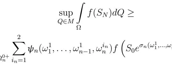
\int \liminfits_{N}\prod_{\substack{i = n + 1\\\Omega_{i}^{0}}}\sum_{i = n + 1}^{N}\psi_{i}(\omega_{1},\ldots ,\omega_{i})\chi_{A}(\omega_{1},\ldots ,\omega_{N})\prod_{i = n + 1}^{N}dP_{i}^{0}(\omega_{i}).\tag{34}

Let us calculate

∫Ωn0χΩn−(ω1,…,ωn−1,ωn1)ψn1(ω1,…,ωn−1,ωn1)μn(ω1,…,ωn−1,ωn1)(A)dPn0(ωn1)+
(35)∫Ωn0χΩn+(ω1,…,ωn−1,ωn2)ψn2(ω1,…,ωn−1,ωn2)μn(ω1,…,ωn−1,ωn2)(A)dPn0(ωn2).

Substituting ψn1(ω1,…,ωn−1,ωn1),ψn2(ω1,…,ωn−1,ωn2) into (35), we obtain

∫Ωn0ψn(ω1,…,ωn−1,ωn)μn(ω1,…,ωn−1,ωn)(A)dPn0(ωn)=
∫Ωn0×Ωn0χΩn−(ω1,…,ωn−1,ωn1)χΩn+(ω1,…,ωn−1,ωn2)×
αn({ω1,…,ωn−1,ωn1};{ω1,…,ωn−1,ωn2})×
[ΔSn+(ω1,…,ωn−1,ωn2)Vn(ω1,…,ωn−1,ωn1,ωn2)μn(ω1,…,ωn−1,ωn1)(A)+
(36)ΔSn−(ω1,…,ωn−1,ωn1)Vn(ω1,…,ωn−1,ωn1,ωn2)μn(ω1,…,ωn−1,ωn2)(A)]dPn0(ωn1)dPn0(ωn2).

From the recurrent relations (23) - (25), we have

μn−1(ω1,…,ωn−1)(A)=∫Ωn0×Ωn0χΩn−(ω1,…,ωn−1,ωn1)χΩn+(ω1,…,ωn−1,ωn2)×αn({ω1,…,ωn−1,ωn1};{ω1,…,ωn−1,ωn2})×[ΔSn+(ω1,…,ωn−1,ωn−1,ωn2)Vn(ω1,…,ωn−1,ωn1,ωn2)μn(ω1,…,ωn−1,ωn1)(A)+
(39)∫∏i=nNΩi0∏i=nNψi(ω1,…,ωi)χA(ω1,…,ωN)∏i=nNdPi0(ωi).

To prove that μ0(ΩN)=1, let us prove the equality

(40)∫Ωn0ψn(ω1,…,ωn)dPn0(ωn)=1,(ω1,…,ωn−1)∈Ωn−1,n=1,N―.

We have

∫Ωn0ψn(ω1,…,ωn)dPn0(ωn)=
∫Ωn0∫Ωn0χΩn−(ω1,…,ωn−1,ωn1)χΩn+(ω1,…,ωn−1,ωn2)×
αn({ω1,…,ωn−1,ωn1};{ω1,…,ωn−1,ωn2})×
[ΔSn+(ω1,…,ωn−1,ωn2)Vn(ω1,…,ωn−1,ωn1,ωn2)+
ΔSn−(ω1,…,ωn−1,ωn1)Vn(ω1,…,ωn−1,ωn1,ωn2)]dPn0(ωn1)dPn0(ωn2)=
∫Ωn0∫Ωn0χΩn−(ω1,…,ωn−1,ωn1)χΩn+(ω1,…,ωn−1,ωn2)×
(41)αn({ω1,…,ωn−1,ωn1};{ω1,…,ωn−1,ωn2})dPn0(ωn1)dPn0(ωn2)=1.

The last equality follows from the fact that the set of random values αn({ω1}n1;{ω1}n2), n=1,N―, satisfies the condition (16). The equalities (40) proves that every measure (27), defined by the set of random values αn({ω11,…,ωn1};{ω12,…,ωn2}), n=1,N―, satisfying the conditions (14), (16), is a probability measure being equivalent to the measure PN.

Further, we also use the probability spaces {Ωn,Fn,μ0n}, n=1,N―, where under the measure μ0n(B),B∈Fn, we understand the measure, given by the formula

(43)μ0n(B)=∫Ωn∏i=1nψi(ω1,…,ωi)χB(ω1,…,ωn)∏i=1ndPi0(ωi),B∈Fn.

Note 2. Assume that for αn({ω11,…,ωn−11,ωn1};{ω12,…,ωn−12,ωn2}), constructed in Lemma 1, the inequalities

0<cn≤αn({ω11,…,ωn−11,ωn1};{ω12,…,ωn−12,ωn2})≤Cn<∞,

are true. Suppose that the conditions

(44)ΔSn−(ω1,…,ωn−1,ωn)≤Bn<∞,n=1,N―,

are valid, where cn, Cn, Bn are constant, then the set of equivalent measures to the measure PN, described in Lemma 2, is nonempty one.

Proof. Due to Lemma 2 conditions, the equality (14) is true. Further,

∫Ωn0∫Ωn0χΩn−(ω11,…,ωn−11,ωn1)χΩn+(ω12,…,ωn−12,ωn2)×
αn({ω11,…,ωn−11,ωn1};{ω12,…,ωn−12,ωn2})×
ΔSn+(ω1,…,ωn−1,ωn2)ΔSn−(ω1,…,ωn−1,ωn1)Vn(ω1,…,ωn−1,ωn1,ωn2)dPn0(ωn1)dPn0(ωn2)≤Bn,
({ω11,…,ωn−11};{ω12,…,ωn−12})∈Ωn−1×Ωn−1,(ω1,…,ωn−1)∈Ωn−1,
∫Ωn0×Ωn0χΩn−(ω11,…,ωn−11,ωn1)χΩn+(ω12,…,ωn−12,ωn2)×
αn({ω11,…,ωn−11,ωn1};{ω12,…,ωn−12,ωn2})dPn0(ωn1)dPn0(ωn2)=1,
(45)({ω11,…,ωn−11};{ω12,…,ωn−12})∈Ωn−1×Ωn−1.
αn({ω1,…,ωn−1,ωn1};{ω1,…,ωn−1,ωn2})×
[ΔSn+(ω1,…,ωn−1,ωn2)Vn(ω1,…,ωn−1,ωn1,ωn2)μnfN(ω1,…,ωn−1,ωn1)+
(46)ΔSn−(ω1,…,ωn−1,ωn1)Vn(ω1,…,ωn−1,ωn1,ωn2)μnfN(ω1,…,ωn−1,ωn2)]dPn0(ωn1)dPn0(ωn2),n=1,N―,
μN−1fN(ω1,…,ωN−1)=∫ΩN0×ΩN0χΩN−(ω1,…,ωN−1,ωN1)χΩN+(ω1,…,ωN−1,ωN2)×
αN({ω1,…,ωN−1,ωN1};{ω1,…,ωN−1,ωN2})×
[ΔSN+(ω1,…,ωN−1,ωN2)VN(ω1,…,ωN−1,ωN1,ωN2)fN(ω1,…,ωN−1,ωN1)+
(47)ΔSN−(ω1,…,ωN−1,ωN1)VN(ω1,…,ωN−1,ωN1,ωN2)fN(ω1,…,ωN−1,ωN2)]dPN0(ωN1)dPN0(ωN2).

From the formula (27) of Lemma 2, it follows that

(48)Eμ0fN=∫ΩN∏n=1Nψn(ω1,…,ωn)fN(ω1,…,ωN−1,ωN)∏i=1NdPi0(ωi)

for every nonnegative FN -measurable random value fN(ω1,…,ωN−1,ωN).

Theorem 1. Suppose that the conditions of Lemma 1 are true. Then, the set of nonnegative random values αn({ω}n1;{ω}n2),n=1,N―, satisfying the conditions

Eμ0|ΔSn(ω1,…,ωn−1,ωn)|=
(49)∫ΩN∏i=1Nψi(ω1,…,ωi)|ΔSn(ω1,…,ωn−1,ωn)|∏i=1NdPi0(ωi)<∞,n=1,N―,
∫Ωn∏i=1nψi(ω1,…,ωi)|ΔSn(ω1,…,ωn−1,ωn)|∏i=1ndPi0(ωi)=
2∫Ωn−1∏i=1n−1ψi(ω1,…,ωi)∫Ωn0∫Ωn0χΩn−(ω1,…,ωn−1,ωn1)χΩn+(ω1,…,ωn−1,ωn2)×
αn({ω1,…,ωn−1,ωn1};{ω1,…,ωn−1,ωn2})×
ΔSn+(ω1,…,ωn−1,ωn2)ΔSn−(ω1,…,ωn−1,ωn1)Vn(ω1,…,ωn−1,ωn1,ωn2)×
(50)dPn0(ωn1)dPn0(ωn2)∏i=1n−1dPi0(ωi),n=1,N―.

Since the conditions of Lemma 1 are true, then the set of bounded random values αn({ω11,…,ωn1};{ω12,…,ωn2}), n=1,N―, constructed in Lemma 1, satisfy the conditions (14) - (16).

From the equality (50) for the set of bounded random values αn({ω}n1;{ω}n2), n=1,N―, satisfying the conditions (14) - (16), we obtain the inequality

∫ΩN∏i=1Nψi(ω1,…,ωi)|ΔSn(ω1,…,ωn−1,ωn)|∏i=1NdPi0(ωi)≤
(51)C∫ΩNΔSn−(ω1,…,ωn−1,ωn1)dPN<∞,n=1,N―,

for a certain constant 0<C<∞. This proves that the set of nonnegative random values αn({ω11,…,ωn1};{ω12,…,ωn2}), n=1,N―, satisfying the conditions (49), is a non empty set.

Let us prove that

∫Ωn0ψn(ω1,…,ωn)ΔSn(ω1,…,ωn)dPn0(ωn)=0,
(52)(ω1,…,ωn−1)∈Ωn−1,n=1,N―.
[−ΔSn+(ω1,…,ωn−1,ωn2)Vn(ω1,…,ωn−1,ωn1,ωn2)ΔSn−(ω1,…,ωn−1,ωn1)+
(53)ΔSn−(ω1,…,ωn−1,ωn1)Vn(ω1,…,ωn−1,ωn1,ωn2)ΔSn+(ω1,…,ωn−1,ωn2)]dPn0(ωn1)dPn0(ωn2)=0,

due to the condition (15).

To complete the proof of Theorem 1, let A belongs to the filtration Fn−1, then A=B×∏i=nNΩi0, where B belongs to the σ -algebra Fn−1 of the measurable space {Ωn−1,Fn−1}. Taking into account the equality (41), (53), we have, due to Foubini theorem,

∫ΩN∏i=1Nψi(ω1,…,ωi)χA(ω1,…,ωN)ΔSn(ω1,…,ωn)∏i=1NdPi0(ωi)=
∫Ωn∏i=1nψi(ω1,…,ωi)χB(ω1,…,ωn−1)ΔSn(ω1,…,ωn)∏i=1ndPi0(ωi)=
∫Ωn−1∏i=1n−1ψi(ω1,…,ωi)χB(ω1,…,ωn−1)∏i=1n−1dPi0(ωi)×
(54)∫Ωn0ψn(ω1,…,ωn)ΔSn(ω1,…,ωn)dPn0(ωn)=0.

The last means that Eμ0{Sn(ω1,…,ωn)|Fn−1}=Sn−1(ω1,…,ωn−1). Since every measure, belonging to the convex linear span of the measures considered above, is a finite sum of such measures, then it is a martingale measure being equivalent to the measure PN. Theorem 1 is proved.

Our aim is to describe this convex span of martingale measures in particular cases.

Definition 1. Let {Ω1,F1} be a measurable space. The decomposition An,k, n,k=1,∞―, of the space Ω1 we call exhaustive one, if the following conditions are valid:

1)An,k∈F1,An,k∩An,s=∅,k≠s,⋃k=1∞An,k=Ω1,n=1,∞―;
  1. the(n+1)-th decomposition is a sub-decomposition of then-th one, that is, for everyj,An+1,j⊆An,kfor a certaink=k(j);

  2. the minimal σ -algebra containing all An,k, n,k=1,∞―, coincides with F1.

Lemma 3. Let {Ω1,F1} be a measurable space with a complete separable metric space Ω1 and Borel σ -algebra F1 on it. Then, {Ω1,F1} has an exhaustive decomposition.

The proof of Lemma 3 see, for example, in [15], [16].

For the proof of integral inequalities, we cannot require the fulfillment for the random values αn({ω11,…,ωn1};{ω12,…,ωn2}), n=1,N―, the condition (15) in the Lemma 4.

Lemma 4. Suppose that Ωn0 is a complete separable metric space, Fn0 is a corresponding Borel σ -algebra on Ωn0, n=1,N―, and the conditions of Lemma 1 are valid. If, on the probability space {Ωn−1,Fn−1,μ0n−1}, for each B∈Fn−1, μ0n−1(B)>0, the nonnegative random value fn(ω1,…,ωn−1,ωn) satisfies the inequality

(55)1μ0n−1(B)∫B∫Ωn0∏i=1nψi(ω1,…,ωi)fn(ω1,…,ωn)∏i=1ndPi0(ωi)≤1,B∈Fn−1,

then the inequality

∫Ωn0ψn(ω1,…,ωn)fn(ω1,…,ωn)dPn0(ωn)≤1,
(56){ω1,…,ωn−1}∈Ωn−1,n=1,N―,

is true almost everywhere relative to the measure Pn−1.

Proof. The metric space Ωn−1 is a complete separable metric space with the metric ρ(x,y)=∑i=1n−1ρi(xi,yi), where x=(x1,…,xn−1),y=(y1,…,yn−1)∈Ωn−1, (xi,yi)∈Ωi0, ρi(xi,yi) is a metric in Ωi0. This means that the metric space Ωn−1 has an exhaustive decomposition {Bmk}m,k=1∞. Suppose that (ω1,…,ωn−1)∈Bm,k for a certain k, depending on m, and there exists an infinite number

Denote Am=Am(ω1,…,ωn−1) those sets Bm,k for which (ω1,…,ωn)∈Bm,k for a certain k, depending on m, and μ0n−1(Am)>0. Then, for every integrable finite valued φn−1(ω1,…,ωn−1)

(58)limm→∞∫Amφn−1(ω1,…,ωn−1)dμ0n−1μ0n−1(Am)=φn−1(ω1,…,ωn−1)

almost everywhere relative to the measure μ0n−1. If to put

φn−1(ω1,…,ωn−1)=
(59)∫Ωn0ψn(ω1,…,ωn)fn(ω1,…,ωn)dPn0(ωn),(ω1,…,ωn−1)∈Ωn−1,

then we obtain the proof of Lemma 4.

In Theorem 2, we assume that for ΔSn(ω1,…,ωn−1,ωn), n=1,N―, the representation

ΔSn(ω1,…,ωn−1,ωn)=
Sn−1(ω1,…,ωn−1)an(ω1,…,ωn−1,ωn)ηn(ωn)=
(60)dn(ω1,…,ωn−1,ωn)ηn(ωn),n=1,N―,S0>0,

is true, where the random values dn(ω1,…,ωn−1,ωn), an(ω1,…,ωn−1,ωn), ηn(ωn), n=1,N―, given on the probability space {Ωn,Fn,Pn}, satisfy the conditions

0<an(ω1,…,ωn−1,ωn)≤1,1+an(ω1,…,ωn−1,ωn)ηn(ωn)>0,
(61)dn(ω1,…,ωn−1,ωn)>0,Pn0(ηn(ωn)>0)>0,Pn0(ηn(ωn)<0)>0.

From these conditions we obtain Ωn− = Ωn0−×Ωn−1, Ωn+=Ωn0+×Ωn−1, where Ωn0−={ωn∈Ωn0,ηn(ωn)≤0}, Ωn0+={ωn∈Ωn0,ηn(ωn)>0}.

From the suppositions above, it follows that Pn0(Ωn0−)>0, Pn0(Ωn0+)>0. The measure Pn0− is a contraction of the measure Pn0 on the σ -algebra Fn0−=Ωn0−∩Fn0, Pn0+ is a contraction of the measure Pn0 on the σ -algebra Fn0+=Ωn0+∩Fn0.

(62)(ω1,…,ωn−1)∈Ωn−1,(ωn1,ωn2)∈Ωn0−×Ωn0+,n=1,N―,

are true almost everywhere relative to the measure Pn−1×Pn0−×Pn0+ on the measurable space {Ωn−1×Ωn0−×Ωn0+,Fn−1×Fn0−×Fn0+}.

Proof. Under Theorem 2 conditions, the set of martingale measures is a nonempty one. Due to the equality (40), we obtain

∫ΩN∏i=1Nψi(ω1,…,ωi)fn(ω1,…,ωn)∏i=1NdPi0(ωi)=
(63)∫Ωn∏i=1nψi(ω1,…,ωi)fn(ω1,…,ωn)∏i=1ndPi0(ωi).

Further,

∫Ωn0ψn(ω1,…,ωn)fn(ω1,…,ωn)dPn0(ωn)=
∫Ωn0∫Ωn0χΩn−(ω1,…,ωn−1,ωn1)χΩn+(ω1,…,ωn−1,ωn2)×
αn({ω1,…,ωn−1,ωn1};{ω1,…,ωn−1,ωn2})×
[ΔSn+(ω1,…,ωn−1,ωn2)Vn(ω1,…,ωn−1,ωn1,ωn2)fn(ω1,…,ωn−1,ωn1)+
(64)ΔSn−(ω1,…,ωn−1,ωn1)Vn(ω1,…,ωn−1,ωn1,ωn2)fn(ω1,…,ωn−1,ωn2)]dPn0(ωn1)dPn0(ωn2).
χΩn−(ω1,…,ωn1)=χΩn−1(ω1,…,ωn−1)χΩn0−(ωn1),
(65)χΩn+(ω1,…,ωn2)=χΩn−1(ω1,…,ωn−1)χΩn0+(ωn2).

is true almost everywhere relative to the measure Pn−1 on the σ -algebra Fn−1. Let us put

(67)αn({ω1,…,ωn−1,ωn1};{ω1,…,ωn−1,ωn2})=αn(ωn1;ωn2),

where αn(ωn1;ωn2) satisfy the condition

(68)∫Ωn0−∫Ωn0+αn(ωn1;ωn2)dPn0(ωn1)dPn0(ωn2)=1.

Since, on the probability space {Ωn0−×Ωn0+,Fn0−×Fn0+,Pn0−×Pn0+}, there exists an exhaustive decomposition {Am,k}m,k=1∞, let us put

(69)αn(ωn1;ωn2)=(1−ε)χAm,k(ωn1;ωn2)μn(Am,k)+εχΩn0−×Ωn0+∖Am,k(ωn1;ωn2)μn(Ωn0−×Ωn0+∖Am,k),

where μn(A)=[Pn0−×Pn0+](A), A∈Fn0−×Fn0+, and we assume that μn(Am,k)>0, μn(Ωn0−×Ωn0+∖Am,k)>0. Suppose that (ωn1;ωn2)∈Am,k and μn(Am,k)>0 for the infinite number of m and k. Then,

∫Ωn0∫Ωn0χΩn0−(ωn1)χΩn0+(ωn2)[(1−ε)χAm,k(ωn1;ωn2)μn(Am,k)+εχΩn0−×Ωn0+∖Am,k(ωn1;ωn2)μn(Ωn0−×Ωn0+∖Am,k)]×
[ΔSn+(ω1,…,ωn−1,ωn2)Vn(ω1,…,ωn−1,ωn1,ωn2)fn(ω1,…,ωn−1,ωn1)+
(70)ΔSn−(ω1,…,ωn−1,ωn1)Vn(ω1,…,ωn−1,ωn1,ωn2)fn(ω1,…,ωn−1,ωn2)]dPn0(ωn1)dPn0(ωn2)≤1.

Going to the limit as m,k→∞ and then as ε→0, we obtain the inequality

χΩn0,−(ωn1)χΩn0,+(ωn2)[ΔSn+(ω1,…,ωn−1,ωn2)Vn(ω1,…,ωn−1,ωn1,ωn2)fn(ω1,…,ωn−1,ωn1)+
(71)ΔSn−(ω1,…,ωn−1,ωn1)Vn(ω1,…,ωn−1,ωn1,ωn2)fn(ω1,…,ωn−1,ωn2)]≤1,(ω1,…,ωn−1)∈Ωn−1,
ΔSn−(ω1,…,ωn−1,ωn1)Vn(ω1,…,ωn−1,ωn1,ωn2)fn(ω1,…,ωn−1,ωn2)]≤1,(ω1,…,ωn−1)∈Ωn−1,

is valid almost everywhere relative to the measure Pn−1×[Pn0×Pn0] on the measurable space {Ωn−1×Ωn0×Ωn0,Fn−1×Fn0×Fn0}.

Proof. Due to the conditions for Ωna, a=−,+, the representation

(73)Ωna=⋃k=1Nn[An0,ka×Vn−1k]

is true. Owing to Lemma 5 conditions, there exists an exhaustive decomposition Dmin, m,i=1,∞―, such that ⋃i=1∞Dmin=Ωn0, m=1,∞―. Let us denote An0,ka∩Dmin=Eminka. It is evident that Eminka forms an exhaustive decomposition of sets An0,ka, n=1,N―, k=1,∞―, a=−,+, correspondingly. Due to Lemma 4, the inequality

(74)∫Ωn0ψn(ω1,…,ωn)fn(ω1,…,ωn)dPn0(ωn)≤1,(ω1,…,ωn−1)∈Ωn−1,

is true almost everywhere relative to the measure Pn−1. The equality

∫Ωn0ψn(ω1,…,ωn)fn(ω1,…,ωn)dPn0(ωn)=
∫Ωn0∫Ωn0χΩn−(ω1,…,ωn−1,ωn1)χΩn+(ω1,…,ωn−1,ωn2)×
αn({ω1,…,ωn−1,ωn1};{ω1,…,ωn−1,ωn2})×
[ΔSn+(ω1,…,ωn−1,ωn2)Vn(ω1,…,ωn−1,ωn1,ωn2)fn(ω1,…,ωn−1,ωn1)+
(75)ΔSn−(ω1,…,ωn−1,ωn1)Vn(ω1,…,ωn−1,ωn1,ωn2)fn(ω1,…,ωn−1,ωn2)]dPn0(ωn1)dPn0(ωn2)
(76)ΔSn−(ω1,…,ωn−1,ωn1)Vn(ω1,…,ωn−1,ωn1,ωn2)fn(ω1,…,ωn−1,ωn2)]dPn0(ωn1)dPn0(ωn2)≤1,

is true almost everywhere relative to the measure Pn−1 on the σ -algebra Fn−1. Let us put

αnr,s−(ω11,…,ωn1)=∑k=1Nnαn,k,r,s−(ωn1)χAn0,k−(ωn1)χVn−1k(ω11,…,ωn−11),
αnm,i+(ω12,…,ωn2)=∑k=1Nnαn,k,m,i+(ωn2)χAn0,k+(ωn2)χVn−1k(ω12,…,ωn−12),
(77)αnr,s,m,i({ω11,…,ωn1};{ω12,…,ωn2})=αnr,s−(ω11,…,ωn1)αnm,i+(ω12,…,ωn2),

where

αn,k,r,s−(ωn1)=[(1−δ)χErsnk−(ωn1)Pn0(Ersnk−)+δχAn0k−∖Ersnk−(ωn1)Pn0(An0k−∖Ersnk−)],
(78)αn,k,m,i+(ωn2)=[(1−δ)χEmink+(ωn2)Pn0(Emink+)+δχAn0k+∖Emink+(ωn2)Pn0(An0k+∖Emink+)],0<δ<1.

In the formulas (78), we assume that the inequalities

(79)Pn0(Ersnk−)>0,Pn0(An0k−∖Ersnk−)>0,Pn0(Emink+)>0,Pn0(An0k+∖Emink+)>0,

are true. Let us consider

αnr,s,m,i({ω1,…,ωn−1,ωn−11};{ω1,…,ωn−1,ωn2})=
(80)αnr,s−(ω1,…,ωn−1,ωn1)αnm,i+(ω1,…,ωn−1,ωn2).

Suppose that (ω1,…,ωn−1)∈Vn−1k for a certain k. Then,

Substituting (81) into (76) and going to the limit as m,k→∞, r,s→∞ and then as δ→0, we obtain the needed inequality. Lemma 5 is proved.

Theorem 3. Suppose that the conditions of Theorem 2 are true. If for a certain ωn1∈Ωn0− and ωn2∈Ωn0+ the inequalities

sup(ω1,…,ωn−1)∈Ωn−11ΔSn−(ω1,…,ωn−1,ωn1)<∞,
(82)sup(ω1,…,ωn−1)∈Ωn−11ΔSn+(ω1,…,ωn−1,ωn2)<∞,n=1,N―,

are true, then the nonnegative random values fn(ω1,…,ωn−1,ωn), n=1,N―, satisfy the inequalities

fn(ω1,…,ωn−1,ωn)≤
(83)(1+γn−1(ω1,…,ωn−1)ΔSn(ω1,…,ωn−1,ωn)),n=1,N―,

where γn−1(ω1,…,ωn−1) is a bounded Fn−1 -measurable random value.

Proof. From the inequality (71), it follows the inequality

fn(ω1,…,ωn−1,ωn2)≤
(84)1+1−fn(ω1,…,ωn−1,ωn1)ΔSn−(ω1,…,ωn−1,ωn1)ΔSn+(ω1,…,ωn−1,ωn2),ωn1∈Ωn0−,ωn2∈Ωn0+.
(85)γn−1(ω1,…,ωn−1)=inf{ωn1,ηn−(ωn1)>0}1−fn(ω1,…,ωn−1,ωn1)ΔSn−(ω1,…,ωn−1,ωn1),

then, taking into account the inequality (84), we obtain the inequality

(86)fn(ω1,…,ωn−1,ωn2)≤1+γn−1(ω1,…,ωn−1)ΔSn+(ω1,…,ωn−1,ωn2).

From the definition of γn−1(ω1,…,ωn−1), we obtain the inequality

(89)γn−1(ω1,…,ωn−1)≥−1ΔSn+(ω1,…,ωn−1,ωn2).

Due to Theorem 3 conditions, we obtain the boundedness of γn−1(ω1,…,ωn−1). The Fn−1 measurability of the random value γn−1(ω1,…,ωn−1) follows from the fact that Ωn0 is separable metric space and infimum is reached on the countable set, which is dense in Ωn0. Theorem 3 is proved.

Theorem 4. Let the conditions of Lemma 5 be valid. If there exist ωn1∈An0k−, ωn2∈An0k+, and the real numbers ak, bk, k=1,Nn―, such that

sup(ω1,…,ωn−1)∈Vn−1k1ΔSn−(ω1,…,ωn−1,ωn1)=akn<∞,
sup(ω1,…,ωn−1)∈Vn−1k1ΔSn+(ω1,…,ωn−1,ωn2)=bkn<∞,k=1,Nn―,n=1,N―,
(90)max1≤n≤Nsup1≤k≤Nnmax{akn,bkn}<∞,

then there exists a bounded Fn−1 -measurable random value γn−1(ω1,…,ωn−1) such that the inequalities

fn(ω1,…,ωn−1,ωn))≤
(91)(1+γn−1(ω1,…,ωn−1)ΔSn(ω1,…,ωn−1,ωn)),n=1,N―,

are true.

Proof. For ωn1∈An0k−, ωn2∈An0k+ and (ω1,…,ωn−1)∈Vn−1k, we have that (ω1,…,ωn−1,ωn1)∈Ωn−, (ω1,…,ωn−1,ωn2)∈Ωn+. Then, from the inequality (72), we obtain the inequality

[ΔSn+(ω1,…,ωn−1,ωn2)Vn(ω1,…,ωn−1,ωn1,ωn2)fn(ω1,…,ωn−1,ωn1)+
(92)ΔSn−(ω1,…,ωn−1,ωn1)Vn(ω1,…,ωn−1,ωn1,ωn2)fn(ω1,…,ωn−1,ωn2)]≤1.

then, taking into account the inequality (93), we have the inequality

(95)fn(ω1,…,ωn−1,ωn2)≤1+γn−1k(ω1,…,ωn−1)ΔSn+(ω1,…,ωn−1</