I. INTRODUCTION
During the regime of Bretton Woods, international monetary system was in gold exchange standard or rather dollar exchange standard because US dollar was convertible with gold and all other currencies were convertible to US dollar. The exchange rate system was fixed rate with adjustable with (\pm 1%) in either side when 1ounce of gold is equal to 35US\(.At Bretton Woods, USA and allied countries rejected Keynes plan and accepted White's plan since USA was the leading and dominant country in the world in terms of international trade, international reserves of gold, capital flows including foreign investment and equity and foreign exchange holdings. Above all, USA was the super power in the world political and military strengths. Therefore, USA could not face any problem to select its currency as key currency to dominate multilateral international payments mechanism.
At 1945, India was a colony and its economy was a meagre 300 billion and that of UK $60 billion. During the Bretton
Woods era, USA was the creditor country to the world and UK was in war-related debt. India and China tried to lead an effort to unilateral transfers as current account so as to pressure convertibility to encash colonial transfer of sterling balance from UK. India's share of sterling balance in 1945 was 45% or £1.51 billion-the equivalent of 200 million of stand by arrangement from IMF. In 1966 June World Bank sanctioned US 300 million. IDA also approved loans of US 642 million in 1967-68 and 1968-69 respectively to India (Srinivas, 2017).
US current account balance was positive but started to decline after 1963 and tend to negative from 1971. The real exchange index of Dollar started to fall and reached at bottom in 1966 and reached at peak in 1969 then fell down. The ratio of reserve to imports were 22 and 204 for USA and UK in 1951 which fell to 19 and 67 in 1965 respectively. UK devalued sterling by in 1949 and 1967. French devalued in 1967. India devalued 1949 and 1966 respectively (Meltzer, 1991). All these results produced the crisis of reserve currencies. USA and IMF created SDR as reserve and international payments for development finance. The cyclical inflation rate was observed during 1950-1971 although trade openness, international trade volume, living standard increased to a larger extent. But, slowly and steadily US but foreign liabilities were 12 billion dollar. On the other hand, in 1967, US gold
stock was 12 billion dollar in comparison with 50 billion US dollar of foreign liabilities. In 1971, US liabilities was 80 billion dollar but US gold stock was only 9 billion dollar (Saderno, 2012). In 1970, oil price shock crumbled down international economy too. In 1971 August, President Nixon was forced to suspend the gold dollar convertibility and ultimately Bretton Woods system collapsed. US hegemony over the international economy started to decline. In 1950, 1960 and 1970 the world share of export of USA were , and respectively and world import share were and respectively in 1960 and 1970. The international share of GDP of USA also started to diminish i.e., in 1950, in 1960, and in 1970 respectively. India's world share of GDP was also declined gradually from in 1950 to in 1960 and in 1970 respectively (Maddison, 2007).
The bulk of US grants, credits and assistance to India from 1945 to 1970 reshuffled Indian economy towards development with deficit finance taking huge loan from IMF, IBRD and IDA etc. Whether these capital inflows have significant relation with US export, import and GDP and India's export and import or not is the important econometric study of this paper during the regime of Bretton Woods.
II. REVIEW OF LITERATURE
Reddy (2000) thought that the relationship between Bretton Woods and India is considered to be mutual benefit through not necessary one of full agreement on many matters. India commands greater respect in Bretton Woods Institutions than any time before for charting its own path towards growth and stability. India's move in Bretton Woods to show and sanction policy of poverty elimination and development in IMF strategy and India wanted to encash convertibility of colonial transfers from U.K. Schuler (2013) also felt similar opinion in the sense that India raised at Bretton Woods on the convertibility of Pound Sterling assets the extent to which the IMF would stress economic development over BOP considerations and quota. Chandavarkar (2001) argued that the role played by Raisman at the Bretton Woods was reflected by India's interest on quota, unilateral payment and policy on development. Simha (1970) thoughtfully explained that India's attitude was bound to be conditioned by special factors such as backwardness, it's appalling poverty, its dismally low standard of living and its just aspirations to make up the long leeway in industrial and agricultural development which should be matched with Bretton Woods developmental plans for major goals. Joshi (1944) acknowledged that India would serve India's interest in international negotiations without being dictated to by Britain. Indian delegates and Raisman echoed in the meeting about RBI's decisions on prioritise development goals, needs of poor countries,
special treatment status, and so on. India rightly considered about to maintain domestic price level than to keep up stable exchange rate. On the other hand, India should be allowed to use tariffs and foreign exchange rationing to protect and strengthen local industry. Joshi objected to the omission of any reference to sterling balances and even in the transitional period. He was positive to adjust exchange rate when India was in fundamental disequilibrium although he was in favour of flexible exchange rate being India as an agricultural country and he was indirectly favour fund's proposal of high level of employment with real income maintenance. Helleiner (2015) opined that Keynes singled out Deshmukh's performance on India's role and remarked that it was brilliant representation. But finally, USA chose to oppose underdeveloped phrase in the charter of IMF rather they wrote economically backward countries. On the contrary, India's initiative encouraged IBRD's development mandate to final charter. After the conference, Deshmukh (1974) highlighted the development orientation of Bretton Woods in a speech to an Indian audience.
Monboit (2008) said that the USA which since 1944 has turned from the world's biggest creditor to the world's biggest debtor, would cause to regret the position it took at Bretton Woods. Following White plan, the IMF insisted that the foreign exchange reserves maintained by other nations are held in the form of dollars. This is one of the reasons why the US economy does not collapse no matter how much debt it accumulates. Eichengreen (2018) rightly remarked that the conference took place at the time of unquestioned US hegemony over the western alliance and the global economy. America had the intellectual and financial resources with which to drive the reform process. Now it lacks both. Moreover, on the process of future Bretton Woods, he said that it would be useful first step toward making the world a safer financial place and it would minimise the danger that New Bretton Woods conference will go down in history as a failure. World Economic and Social Survey (2017) assessed that Bretton Woods era is the golden age of capitalism when growth of international trade was unprecedented and was created a multilateral international payment system known as Bretton Woods Monetary System and was a positive attempt to aid Europe through Marshall Plan which was a positive experience of development cooperation with successful implementation of sustainable development goal. Marshall plan which accounts of GNP restored productive capacity in western Europe, improved price stability and helped their currencies in post war period. Even, USA started a package of development programme in developing countries through Official Development Assistance (ODA) which accounts of GNI which increased to of GNI from 1960. But volatile commodity price and declining prices of primary products remained unsolved
issues today. During Bretton Woods, structural imbalance in trade between developed and developing countries, gap of foreign exchange earnings, technological change and competitive devaluation were observed and due to devaluation in UK in 1949 and 1967, devaluation in France in 1967 and declined US gold reserve with negatively moving current account ultimately broke down Bretton Woods system.
Balasubrahmonian (n.d.) stated that India's reserves position dropped precipitously from 1947 onwards which forced to draw 122.5m from the IMF during 1961-2 and 800m) that were utilised as infrastructural development and transportation.
India's Five-Year Plans depended on deficit financing to be plugged by foreign aid. The ratio of foreign aid to new private capital investment between 1948 and 1961 was 6:1. One of the largest donors to India was the United States, which contributed between 1954 and 1967 including (3.8bn of PL480 food aid which allowed India to focus Plan expenditures on heavy industry development.
In the 1960s, these dynamics began to shift. American dollar hegemony began to come under strain as the fixed exchange rate regime came under pressure. By 1961, America had abandoned the policy of local currency repayment for dollar loans. The troika of the United States, the World Bank and the IMF, sought to persuade India to devalue, liberalise, imports and gave higher priority to agriculture. This was characterised as the Bank's most significant attempt to use the leverage of its lending to modify macroeconomic policies in a major member country. During mid-1960s, debt multilateralization mediated through the IMF and World Bank had virtually taken place. The bilateral aid relationship between India and America had come under strain, not merely because of the pressure on American gold reserves and the diminished agricultural surplus, but also because of India's rather vocal discomfort with the Vietnam War and her status as leader of the Non-Aligned World. The crisis in India's Five-Year Planning came on the heels of the suspension of American aid during the 1965 War with Pakistan.
Balasubrahmanian (2018) also reminds us that VKRVRao acknowledged the benefits of signing the Bretton Woods agreements but showed three serious defects from the view point of India, such as [i] the failure to include wartime balances within the scope of the fund,[ii] the small size of the quota allotted to India and [iii] the failure to receive a permanent seat on the Executive Board of the Fund. Moreover, on the question of sterling balance BalaSubrahmanian remarked that ultimately, India -UK bilateral agreement settled India's
sterling balances where as the dis-satisfaction remains between India and Bretton Woods resolution.
Sato (2010) argued that during Bretton Woods period, India followed fixed exchange rate with US dollar facing huge balance of payments deficit acutely two times during 1952-57 and 1965-66 amounting to of GDP and even India faced bulk of fiscal deficit for development finance in which India took external finance as aid, debt finance and equity for payments management in terms of external borrowing, NRI deposits and equity finance as foreign direct and portfolio investments. India's capital inflows reached at peak of of GDP in 1965 where USA played the leading role.
III. SOURCE OF DATA AND METHODOLOGY
The paper assumed: exports in billion US 1,234{2} =$ 1,234{1} =$ 1,234 =$ 1,234 =$ 1,234 =$ 1,234$ in current prices. Data have been collected from US Bureau of Economic Research, United Nations Conference on Trade and Development and https://shodhganga.infilbnet.ac.in/bitstream/10603/171552/14/12_chapter%2002pdf.
Linear and non-linear trend lines were calculated by applying the semi-log regression model. The structural breaks have been found out by using Bai-Perron Model (2003). Decomposition of trend and cycle was shown by utilising Hodrick Prescott Filter Model (1997). Even, Hamilton filter model (2018) has been applied for finding cycles, trends and seasonal variations. Cointegration test was done by following the Johansen model (1988). Vector Error Correction Model was also analysed through the Johansen model (1991). Short run causality was checked by the Wald Test (1943). Hansen-Doornik Normality test (1994) was used to show residual test of normality of the Vector Error Correction Model. Long run causality was verified by cointegration equation.
IV. OBSERVATIONS FROM MODELS
[i] Nature of Trends
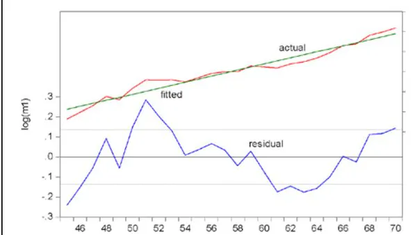
US grants, credits and assistance in India during Bretton Woods era from 1945 to 1970 have been catapulting at the rate of per year significantly.
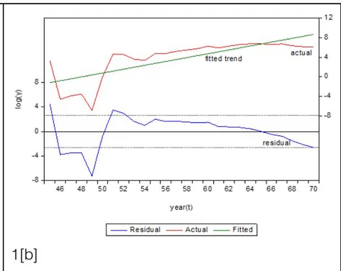
R^{2}=0.57, F=32.17^{\star}, DW=0.88, y=US \text{grants, credits and assistance in India (million US)}, t=\text{year}^{\star}=$
significant at level, random error. The steady trendline is plotted in Figure 1[b]. In fact, its trend should be non-linear with increasing in the first phase and decreasing in the second phase significantly which is estimated as below:
, , , random error, significant at level. The non-linear estimated trend line is depicted in Figure 1A below which is stable according to stability test of recursive residuals.
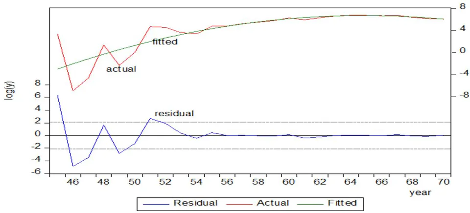
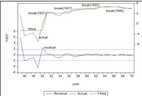
Bai-Perron test for structural breaks using HAC standard errors & covariance found four structural breaks in y in which upward breaks were seen in 1951,
1957, 1963 and downward structural break was seen in 1968. All of which are significant. Details of structural breaks are given in Table-1.
| Variable | Coefficient | Standard Error | t-Statistic | Probability |
| 1945 - 1950 -- 6 observations | ||||
| C | -2.594035 | 1.246351 | -2.081304 | 0.0498 |
| 1951 - 1956 -- 6 observations | ||||
| C | 4.292241 | 0.235640 | 18.21526 | 0.0000 |
| 1957 - 1962 -- 6 observations | ||||
| C | 5.825674 | 0.211089 | 27.59817 | 0.0000 |
| 1963 - 1967 -- 5 observations | ||||
| C | 6.697476 | 0.015874 | 421.9177 | 0.0000 |
| 1968 - 1970 -- 3 observations | ||||
| C | 6.191113 | 0.061442 | 100.7634 | 0.0000 |
| R2=0.82, F=24.63, DW=1.89 |
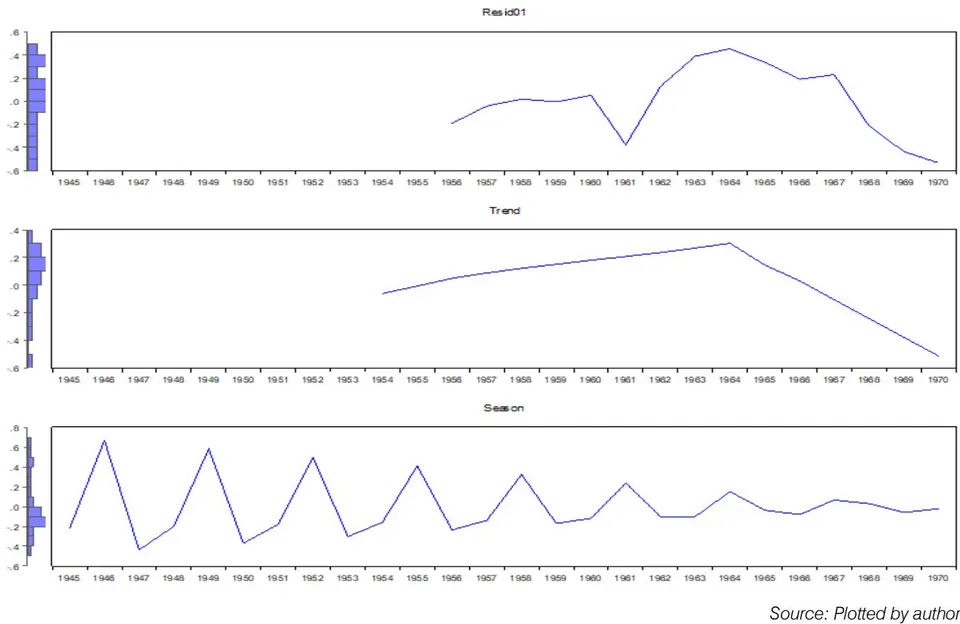
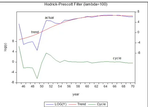
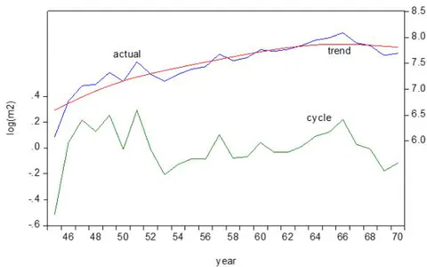
In Figure 2[b] the structural breaks are plotted clearly. Hodrick-Prescott Filter of US grants and credit during 1945-1970 assured long run upward trend and cycles with four peaks and troughs assuming . It is seen in the figure 3[b] But Hamilton filter model (2018) confirmed by decomposing into trend, cycles and seasonal variation that the US grants to India showed three peaks and two troughs, one upward and downward trends and a
seasonal variation spreading throughout the period from 1945-1970. In panel 1 the cycles, in panel 2, the trend and in panel 3, the seasonal variations were clearly plotted in the Figure 1B below.
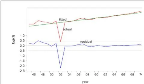
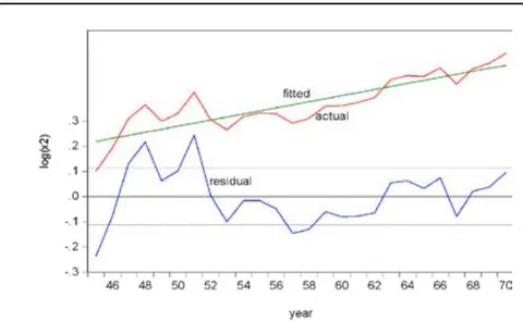
US exports (in billion US$) has been increasing at the rate of 6.18% per year during Bretton Woods era significantly.
R²=0.506, F=24.58*, DW=2.01, x₁= US exports in billion US$, t=year, *=significant at 5% level,
random error. This trendline is observed in Figure 1[c].
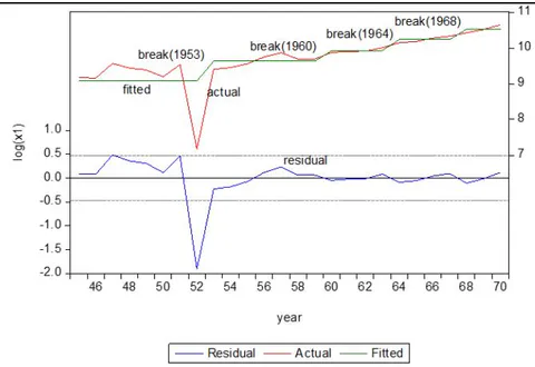
U.S. exports consists of four upward structural breaks in 1953, 1960, 1964 and 1968 respectively which were found from Bai-Perron model. In Table 2 the values of co-efficients, t statistic and probabilities have been arranged.
| Variable | Coefficient | Standard Error | t-Statistic | Probability |
| 1945 - 1952 -- 8 observations | ||||
| C | 9.077395 | 0.272974 | 33.25364 | 0.0000 |
| 1953 - 1959 -- 7 observations | ||||
| C | 9.632027 | 0.085901 | 112.1290 | 0.0000 |
| 1960 - 1963 -- 4 observations | ||||
| C | 9.924247 | 0.027029 | 367.1641 | 0.0000 |
| 1964 - 1967 -- 4 observations | ||||
| C | 10.23312 | 0.043563 | 234.9040 | 0.0000 |
| 1968 - 1970 -- 3 observations | ||||
| C | 10.52716 | 0.047858 | 219.9649 | 0.0000 |
| R2=0.589, F=7.53, DW=1.96 |
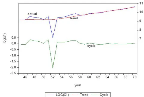
Even in the Figure 2[c] the structural breaks are seen distinctly. In the long term trend one downward trend was observed during the complete upward trend from 1945 to 1970 where three peaks and troughs were clearly visible in analysing the H.P.Filter model which is plotted in the Figure 3[c].
Indian exports (in million Rupees) has been stepping up at the rate of per year during 1945-1970 significantly.
.
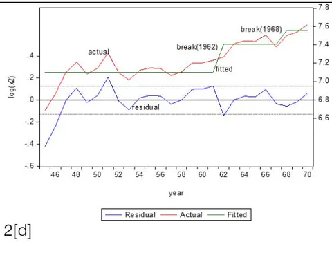
Indian exports showed two upward structural breaks in 1962 and 1968 respectively which are significant. All values have been given in Table-3. Moreover, in Figure 2[d], the structural breaks of Indian exports are visibly seen neatly.
| Variable | Coefficient | Standard Error | t-Statistic | Probability |
| 1945 - 1961 -- 17 observations | ||||
| C | 7.102809 | 0.043301 | 164.0339 | 0.0000 |
| 1962 - 1967 -- 6 observations | ||||
| C | 7.408435 | 0.031426 | 235.7420 | 0.0000 |
| 1968 - 1970 -- 3 observations | ||||
| C | 7.555521 | 0.025241 | 299.3354 | 0.0000 |
| R2=0.675, F=23.907, DW=0.94 |
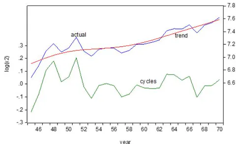
In the H.P.Filter model, Indian exports during 1945-1970 had one long run downward trend during the upward trend where six peaks and troughs were found in the long run cycle. In Figure 3[d] the cycles and trend are clearly seen.
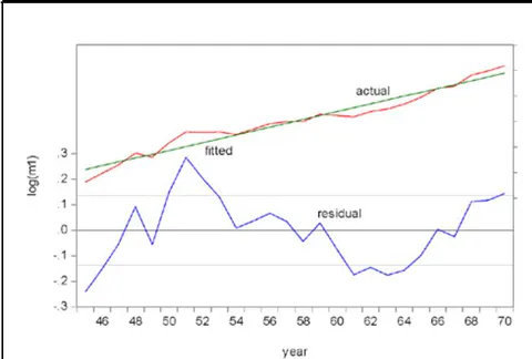
US imports (in million US$) during the course of Bretton Woods era have been rising at the rate of 7.56% per year significantly.
(R^{2} = 0.95) (F = 457.91^{\star}), DW=0.50, (\mathsf{m}_{\mathsf{i}} = ) imports in million US\(, t=year,*=significant at (5 %) level, u=random error. It is clearly plotted in Figure 1[e].
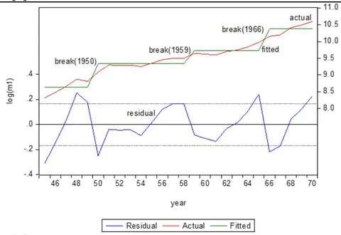
US imports have three strong upward structural breaks in 1950, 1959 and 1966 respectively where all the breaks are significant. All values have been tabulated in Table-4.
| Variable | Coefficient | Standard Error | t-Statistic | Probability |
| 1945 - 1949 -- 5 observations | ||||
| C | 8.627016 | 0.074478 | 115.8326 | 0.0000 |
| 1950 - 1958 -- 9 observations | ||||
| C | 9.336330 | 0.055513 | 168.1833 | 0.0000 |
| 1959 - 1965 -- 7 observations | ||||
| C | 9.731028 | 0.062946 | 154.5942 | 0.0000 |
| 1966 - 1970 -- 5 observations | ||||
| C | 10.36985 | 0.074478 | 139.2332 | 0.0000 |
| R²=0.93, F=98.64, DW=1.21 |
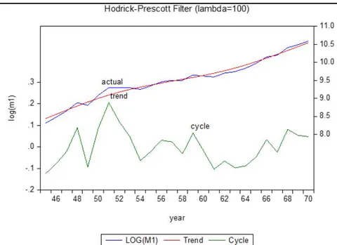
In the long run trend of US imports, there are one downward trend and one upward trend having seven peaks and six troughs during long run cycles under Bretton Woods era which is plotted in Figure3[e].
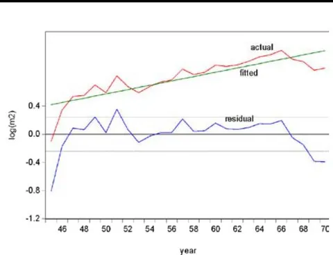
Indian imports (in million Rupees) have been stepping up at the rate of per year significantly during 1945-1970.
( = 0.706) (F = 57.74^{\star}), DW=0.719, (2 =) Indian imports in million US\(, t=year, )*( = significant at (5 %) level, (u{i} =) random error. This trendline is seen in Figure 1[f].
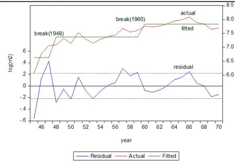
Indian imports during 1945-1970 showed two upward structural breaks significantly in 1948 and 1960 respectively. All the breaks are clearly shown in Table-5. Moreover, the structural breaks have been plotted in the Figure 2[f].
| Variable | Coefficient | Standard Error | t-Statistic | Probability |
| 1945 - 1947 -- 3 observations | ||||
| C | 6.637074 | 0.203941 | 32.54414 | 0.0000 |
| 1948 - 1959 -- 12 observations | ||||
| C | 7.374708 | 0.071756 | 102.7744 | 0.0000 |
| 1960 - 1970 -- 11 observations | ||||
| C | 7.839227 | 0.056555 | 138.6125 | 0.0000 |
| R²=0.77, F=38.77, DW=1.539 |
In H.P.Filter model, Indian imports have steady upward trend path but in the cycles there are six peaks and troughs in the long run which were significant. This is plotted in Figure 3[f].
Gross national income of USA (in million US5.99%$ per year significantly.
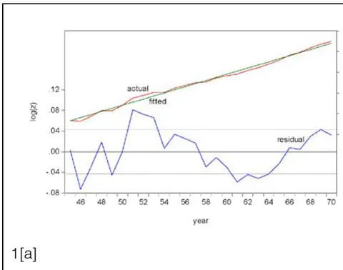
Gross National Income of USA (in million US\star =5%u_{i} =$ random error. The trendline is shown by Figure 1[a].
Gross national income of USA had three upward structural breaks in 1951, 1959 and 1965 significantly as seen by Bai-Perron model. The values of breaks have been arranged in Table-6. Even, the structural breaks have been plotted in Figure 2[a].
| Variable | Coefficient | Standard Error | t-Statistic | Probability |
| 1945 - 1950 -- 6 observations | ||||
| C | 12.38944 | 0.048447 | 255.7309 | 0.0000 |
| 1951 - 1958 -- 8 observations | ||||
| C | 12.86459 | 0.041956 | 306.6175 | 0.0000 |
| 1959 - 1964 -- 6 observations | ||||
| C | 13.21049 | 0.048447 | 272.6784 | 0.0000 |
| 1965 - 1970 -- 6 observations | ||||
| C | 13.62577 | 0.048447 | 281.2501 | 0.0000 |
| R²=0.94, F=118.25, DW=1.25 |
The long run trend of the US National income from 1945 to 1970 is seen as steadily upward but the cyclical path constitutes seven peaks and troughs
respectively which were observed by H.P.Filter model. The cycles and trend are clearly observed in Figure 3[a].
![Figure 1: Growth Rates 2[a]](https://doc.globaljournals.org/zvdm80_61432/ocr/images/derivatives/2d/2d1fb7fa285fff2a08c1c1b9ba3fff8171808e040cb2715849d579e79245f7bf.webp)
![Figure 2: Structural Breaks 3[a]](https://doc.globaljournals.org/zvdm80_61432/ocr/images/derivatives/f7/f7f2b168c043f09297507b07aac7e9255d36e7c99ed31c4f3a60d49c00628950.webp)


3[f]
Source: Plotted by author
[ii] Analysis of Cointegration and Vector Error Correction Model
Johansen unrestricted rank test of the first difference series of US grants, credits and assistance to India (logy), US exports and imports , Indian exports and imports and US gross
national income (logz) (assuming linear deterministic trend) during 1945-1970 confirmed that Trace statistic and Max-Eigen statistic have three cointegrating equations each which are significant at level. All the values have been arranged in the Table 7.
| Hypothesized No. of CE(s) | Eigenvalue | Trace Statistic | 0.05 Critical Value | Probability.** |
| None * | 0.988933 | 209.5674 | 95.75366 | 0.0000 |
| At most 1 * | 0.873876 | 101.4756 | 69.81889 | 0.0000 |
| At most 2 * | 0.726799 | 51.78388 | 47.85613 | 0.0204 |
| At most 3 | 0.473833 | 20.64271 | 29.79707 | 0.3803 |
| At most 4 | 0.191834 | 5.231419 | 15.49471 | 0.7838 |
| At most 5 | 0.004976 | 0.119726 | 3.841466 | 0.7293 |
| Hypothesized No. of CE(s) | Eigenvalue | Max-Eigen Statistic | 0.05 Critical Value | Prob.** |
| None * | 0.988933 | 108.0919 | 40.07757 | 0.0000 |
| At most 1 * | 0.873876 | 49.69168 | 33.87687 | 0.0003 |
| At most 2 * | 0.726799 | 31.14117 | 27.58434 | 0.0167 |
| At most 3 | 0.473833 | 15.41129 | 21.13162 | 0.2611 |
| At most 4 | 0.191834 | 5.111693 | 14.26460 | 0.7276 |
| At most 5 | 0.004976 | 0.119726 | 3.841466 | 0.7293 |
The regression equations of the error correction model stated that [i] is positively related with , and significantly and is negatively related with significantly. Two cointegrating equations tend to equilibrium significantly [ii] is positively related with significantly and three error corrections have been moving equilibrium. [iii] is affected positively with , , , and negatively related with
significantly. [iv] is affected positively with and negatively with , and respectively at significant level of . Two cointegrating equations have been marching divergent [v] is positively related with significantly and all error corrections terms have been moving convergent insignificantly. All the values have been arranged in the Table 8 neatly.
| Δlogyt | Δlogx1 | Δlogx2 | Δlogm1 | Δlogm2 | Δlogz1 | |
| CointEq1 | -0.919410 | -0.138362 | -0.052019 | -0.034675 | 0.053072 | -0.012815 |
| t | [-2.91373]* | [-2.13840]* | [-4.35131]* | [-1.74748] | [2.64200]* | [-1.82942] |
| CointEq2 | -2.184286 | -1.234668 | -0.202720 | -0.001922 | 0.204627 | -0.034264 |
| t | [-1.30870] | [-3.60755]* | [-3.20587]* | [-0.01831] | [1.92584] | [-0.92478] |
| CointEq3 | -13.19885 | -2.989674 | -0.866915 | -0.458562 | 0.755106 | -0.194131 |
| t | [-2.56454]* | [-2.83289]* | [-4.44600]* | [-1.41685] | [2.30467]* | [-1.69919] |
| Δlogyt-1 | 1.127690 | 0.076964 | 0.053819 | 0.036208 | 0.012207 | 0.017260 |
| t | [3.71492]* | [1.23646] | [4.67966]* | [1.89679] | [0.63170] | [2.56137]* |
| Δlogyxt-1 | 0.767305 | -0.089338 | 0.079794 | -0.034335 | -0.024764 | -0.005851 |
| t | [1.08034] | [-0.61342] | [2.96541]* | [-0.76874] | [-0.54769] | [-0.37111] |
| Δlogyxt-1 | 0.083100 | 0.164712 | 0.187206 | -0.012184 | -0.703254 | 0.110115 |
| t | [0.01543] | [0.14911] | [0.91724] | [-0.03596] | [-2.05060]* | [0.92079] |
| Δlogm1t-1 | 4.369679 | 2.647903 | 0.486588 | 0.074579 | 1.787153 | 0.147939 |
| t | [0.73351] | [2.16765]* | [2.15594]* | [0.19908] | [4.71241]* | [1.11869] |
| Δlogm2t-1 | 7.022404 | -0.415770 | 0.217290 | 0.168567 | -0.361965 | 0.074068 |
| t | [2.69673]* | [-0.77864] | [2.20248]* | [1.02938] | [-2.18346]* | [1.28131] |
| Δlogz1t-1 | -47.18023 | -2.425637 | -1.616675 | -0.842372 | -3.810986 | -0.721121 |
| t | [-2.71297]* | [-0.68021] | [-2.45373]* | [-0.77027] | [-3.44229]* | [-1.86794] |
| C | 2.319524 | -0.011090 | 0.055371 | 0.120396 | 0.160433 | 0.084940 |
| t | [2.63784]* | [-0.06151] | [1.66207] | [2.17728]* | [2.86596]* | [4.35143]* |
Source: Calculated by author
By applying Wald test on the system equations of the VECM regression equations, it was observed some short run causalities in the following fashion: US grants, credits and assistance to India have short run causalities from India's imports and US gross national income whose Chi-square(1) value is rejected from causality. In the similar way, causality of US
export from US import, causality from US grants, credits and assistance, US imports, Indian imports and US gross national income to Indian exports, causality from US gross national income to Indian imports and short run causality from US grants, credits and assistance to US gross national income were observed significantly.
| Short run causality from ....to.... | Chi-square(1) | Probability | H0=no causality | Sig/insig |
| Causality from Δlogm2t-1 to Δlogyt | 7.2723 | 0.007 | rejected | significant |
| Causality from Δlogz1t-1 to Δlogyt | 7.3601 | 0.0067 | rejected | Significant |
| Causality from Δlogm1t-1 to Δlogx1t | 4.698 | 0.0302 | rejected | Significant |
| Causality from Δlogyt-1 to Δlogx2t | 4.6312 | 0.0301 | rejected | Significant |
| Causality from Δlogm1t-1 to Δlogx2t | 4.6480 | 0.0311 | rejected | Significant |
| Causality from Δlogm2t-1 to Δlogx2t | 4.8509 | 0.0276 | rejected | Significant |
| Causality from Δlogz1t-1 to Δlogyx2t | 6.0207 | 0.0141 | rejected | Significant |
| Causality from Δlogz1t-1 to Δlogm2t | 11.849 | 0.0006 | rejected | Significant |
| Causality from Δlogyt-1 to Δlogz1 | 6.5606 | 0.0104 | rejected | Significant |
Three normalised cointegrating equations are as follows.
| Cointegrating Equation | CointEq1 | CointEq2 | CointEq3 |
| 1.000000 | 0.000000 | 0.000000 | |
| 0.000000 | 1.000000 | 0.000000 | |
| 0.000000 | 0.000000 | 1.000000 | |
| -256.3150 | -16.28028 | 20.42067 | |
| t | [-8.88832]* | [-8.13604]* | [9.27763]* |
| -85.46583 | -6.110907 | 6.773430 | |
| t | [-5.79156]* | [-5.96780]* | [6.01358]* |
| 353.3942 | 22.25599 | -29.15125 | |
| t | [8.37491]* | [7.60104]* | [-9.05106]* |
| C | -1519.563 | -98.35036 | 126.7701 |
Taking into account of the system equations, the cointegrating equations turned into the following forms.
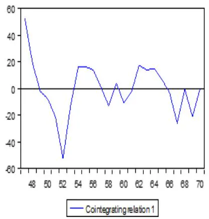
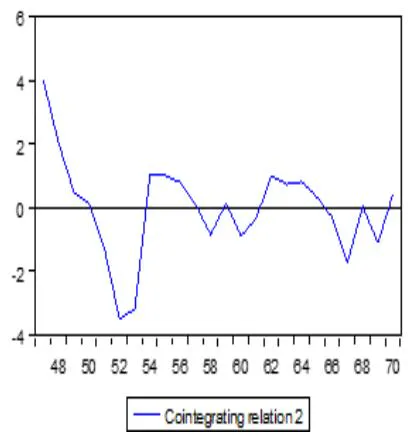
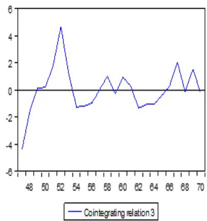
In the first cointegrating equation, it was established that there were long run causalities to US credits, grants and assistance to India from both imports of India and USA and from gross national income of USA during the Bretton Woods era significantly and since all t values of coefficients were significant and coefficient of was negative and significant, it means that the cointegrating equation
moves to the equilibrium or convergent. In the same token, US export had significantly long run causal relationships from US and Indian imports and US gross national income and this equation tended to equilibrium. Similarly, US export had long run causal relations with US and Indian imports and US gross national income and the cointegrating equation was convergent.
In the Figure 4, the cointegrating relationships have been plotted neatly.
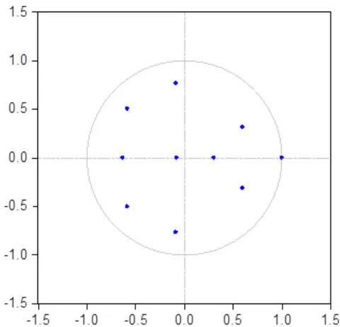
Above all, the model consists of 6 imaginary roots, two negative roots and one root is less than one, two roots are greater than one and one root is unity respectively. Therefore, the model is non-stationary. Besides, one root lies on outside the unit circle and
others lie inside the unit circle which are shown in the Figure 5 which confirms that the model is unstable.
| Root | Modulus |
| 1.000000 | 1.000000 |
| 1.000000 - 1.20e-15i | 1.000000 |
| 1.000000 + 1.20e-15i | 1.000000 |
| -0.085857 - 0.768798i | 0.773578 |
| -0.085857 + 0.768798i | 0.773578 |
| -0.584303 - 0.503332i | 0.771202 |
| -0.584303 + 0.503332i | 0.771202 |
| 0.597528 - 0.314799i | 0.675380 |
| 0.597528 + 0.314799i | 0.675380 |
| -0.632088 | 0.632088 |
| 0.302643 | 0.302643 |
| -0.077931 | 0.077931 |
Source:Calculated by author
Inverse Roots of AR Characteristic Polynomial
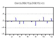
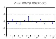
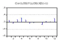
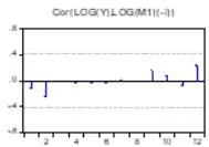
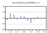
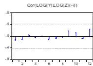
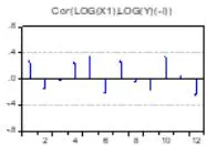
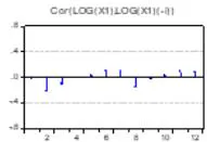
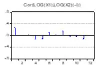
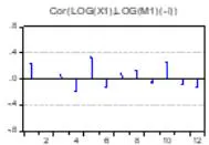
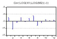
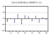
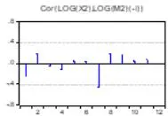
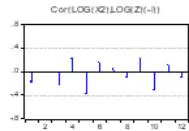
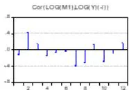
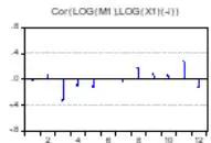
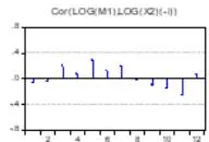
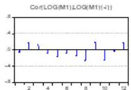
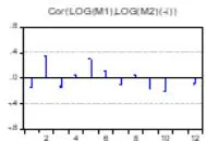
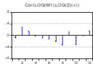
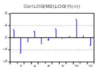
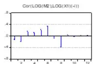
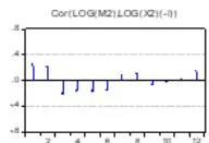
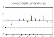
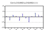
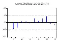
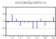
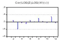
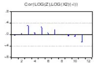
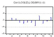
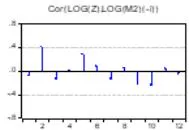
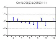
The residual test showed that the model contains problem of autocorrelation which were shown in the Figure 6 where vertical bars move on both the sides. So, there are seasonal variation too.
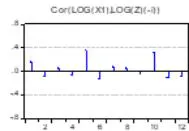
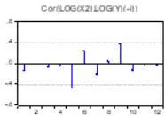
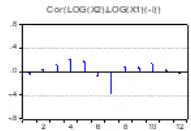
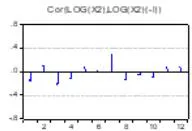
Hansen-Doornik Vector Error Correction residual normality test verified that only component 2 of the Chi-square value of skewness is rejected for
normality but all other values of kurtosis and Jarque-Bera are accepted for normality.
| Component | Skewness | Chi-square | Degree of freedom | Probability |
| 1 | -0.226283 | 0.292548 | 1 | 0.5886 |
| 2 | -0.880496 | 3.849867 | 1 | 0.0497 |
| 3 | -0.373644 | 0.782211 | 1 | 0.3765 |
| 4 | -0.135275 | 0.105336 | 1 | 0.7455 |
| 5 | -0.114754 | 0.075891 | 1 | 0.7829 |
| 6 | -0.519435 | 1.470931 | 1 | 0.2252 |
| Joint | 6.576784 | 6 | 0.3618 | |
| Component | Kurtosis | Chi-square | Degree of freedom | Probability |
| 1 | 3.644874 | 3.465186 | 1 | 0.0627 |
| 2 | 2.960164 | 1.726110 | 1 | 0.1889 |
| 3 | 3.516051 | 2.174090 | 1 | 0.1404 |
| 4 | 2.545372 | 0.062207 | 1 | 0.8030 |
| 5 | 3.383664 | 2.563333 | 1 | 0.1094 |
| 6 | 2.768483 | 0.008646 | 1 | 0.9259 |
| Joint | 9.999573 | 6 | 0.1247 | |
| Component | Jarque-Bera | Degree of freedom | Probability | |
| 1 | 3.757734 | 2 | 0.1528 | |
| 2 | 5.575977 | 2 | 0.0615 | |
| 3 | 2.956301 | 2 | 0.2281 | |
| 4 | 0.167543 | 2 | 0.9196 | |
| 5 | 2.639224 | 2 | 0.2672 | |
| 6 | 1.479578 | 2 | 0.4772 | |
| Joint | 16.57636 | 12 | 0.1662 |
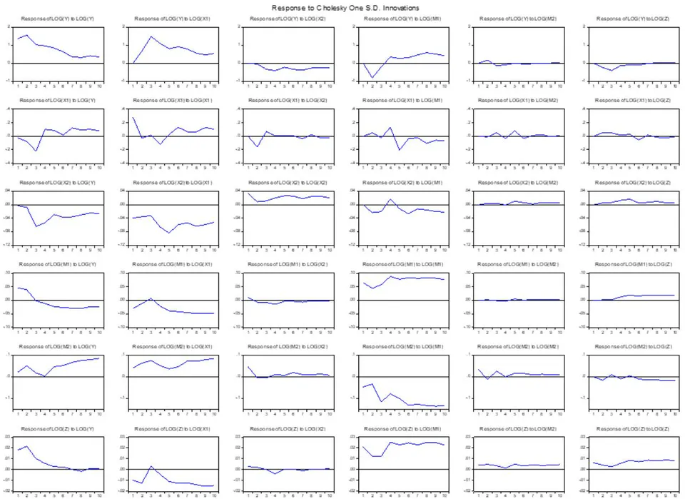
The impulse response functions assumed Cholesky one standard deviation innovations which expressed that the responses of to and , responses of to and , responses of to , response of to
, response of to , response of to and response of to have been moving toward equilibrium which are observed in the Figure 7.
V. LIMITATIONS AND FUTURE SCOPE OF RESEARCH
The model described here suffers from some limitations too. If the variables like, balance of trade, inflation rate, exchange rate of Rupee could be taken into account, then the more viable results might be obtained. Thus, the paper assures enough scope for further research in the offing.
VI. CONCLUSION
The paper concludes that US grants, credits and assistance to India during 1945-1970 had been growing at the rate of per year significantly which had three upwards structural breaks with long run upward cyclical trend and seasonal variations. The upward structural breaks with upward cyclical filter along with high growth rates were also seen from exports and imports of USA and India and from National income of USA during 1945-1970. US grants, credits and assistance to India during 1945-1970 had three significant cointegrating equations with exports and imports of USA and India and national income of USA. The vector error correction model is unstable, nonstationary and non-normal having problem of autocorrelation. US grants, credits and assistance to India have short run causalities from India's imports and US gross national income. There were long run causalities to US credits, grants and assistance to India from both imports of India and USA and from gross national income of USA during the Bretton Woods era significantly.
ACKNOWLEDGMENT
In preparing this paper, I am indebted to all sources of references, the authority of the journal and other well-wishers. I declare that no organisation/NGO/institution have sanctioned the funds to publish this work. I am responsible for all errors and omissions.
Conflict of Interest
There is no conflict of interest in the process of the paper publication.
Bio-Note: MA in Economics, Ph.D. in Economics. Published 12 books, Co-edited 2 books, Edited 2 books, Published more than 220 articles in national and international journals and in edited books.