## I. INTRODUCTION Self-organizing neural maps, also known as competitive neural networks, are an important class of neural networks. These networks focus on two key aspects: the ability to store desired patterns as stable equilibrium points and the mutual interference between neuron and learning dynamics. This research examines how cortical cognitive maps work by using a self-organizing map with differential equations for neural activity levels, short-term memory (STM), and synaptic information efficiency, long-term memory (LTM). STM and LTM models are usually based on classical Grossberg's approach or Amari's model for primitive neural competition [1, 2]. These models often involve mutually inhibitory neurons with fixed synaptic connections [3, 4, 1]. Researchers have studied competitive neural systems using flow invariance theory and singular perturbation theory on large-scale networks. These networks have two types of state variables that describe the slow unsupervised dynamics of synapses and the fast dynamics of neural activity. The fast dynamics are usually represented by the goal of the self-organizing map, such as clustering or recognition. One example is the Willshaw-Malsburg model [1, 5] of topographic formation, which uses solutions of equations of synaptic self-organization coupled with the field equation of neural excitations to improve the understanding of the dynamics of cortical cognitive maps [4, 6]. However, the design using classical competitive differential equations is not broad enough because the synaptic efficiency is not dependent on entropy. Therefore, this paper extends these approaches to incorporate systems where external stimuli can modify the synaptic information efficiency. This is done by estimating the entropy of information transfer between neurons. In other words, this research focuses on LTM in terms of how information transfer evolves. Fractional differential equations are used to model synaptic efficiency based on entropy estimation, which accurately improves the models based on STM and LTM approaches [7, 8, 9, 10, 11]. The study proposes an alternate model for information transfer between neurons based on entropy. It applies McMillan-Shannon's approach to fractional competitive differential equations to determine the mathematical conditions for when STM and the estimation of entropy related to LTM have bounded trajectories. The study uses an alternative version of Lyapunov functions to examine exponential stability in fractional-order systems [7]. This proposal is more comprehensive than previous studies, such as those conducted by [3, 4, 1, 8]. It presents a strict Lyapunov function for the neural multi-time scale system, which demonstrates the existence and uniqueness of the equilibrium point. Additionally, this proposal provides some conditions for global exponential stability based on singular perturbation theory and variable entropy-dependent synaptic efficiency. The paper is structured as follows: In Section 2, the mathematical background related to self-organizing maps modeled by Caputo derivatives is presented. This allows for the inclusion of fractional order in the differential equations associated with STM and LTM dynamics. Section 3 analyzes the equilibrium point from the perspective of synaptic efficiency, and covers the existence and uniqueness of the equilibrium point. Section 4 presents numerical simulations that provide findings about SOM's equilibrium point and entropy when exposed to external stimulus. Finally, Section 5 offers closing remarks and final comments. ## II. MATHEMATICAL BACKGROUND The synaptic information efficiency (SIE) can be defined according to the existence of an ergodic process related to binned input and output spike trains whose length is $N$ bins [4]. In computational experiments, $N$ is associated with iterations during the learning procedure on time domain. In this way, by assuming $m_{ij}$ the synaptic efficiency between $i$ -th and the $j$ -th neuron then let $S_{in}, S_{out}$ the binned input and output spike trains, respectively, both defined by $\{\sigma_1, \ldots, \sigma_N\}$, where $\sigma_i \in \{0,1\}$ represents $i$ -th bin, and assume that this string is the realization of a stationary and ergodic stochastic process. By using the Shannon-MacMillan-Brieman's theorem [12, 13] $-\frac{1}{N} \log_2 p(\sigma_1, \ldots, \sigma_N) \to H$, where $H$ is the entropy rate of $X$ (events set) and $p(\sigma, \ldots, \sigma_N)$ is the probability of obtaining the string $(\sigma_1, \ldots, \sigma_N)$ as a realization of $X$. In that sense, the estimate for the entropy at $N$ -th iteration will be represented by $\hat{H}_N = -\frac{1}{N} \log_2 \hat{p}(\sigma_1, \ldots, \sigma_N)$. So, for $i$ -th neuron, $$ \begin{array}{l} \mathrm {S I E} _ {i} = \hat {H} _ {N} (\sigma_ {1}, \dots , \sigma_ {N}) _ {i} - \hat {H} _ {N} (\sigma_ {1}, \dots , \sigma_ {N} | S _ {i n}) _ {i} \\= \frac {1}{N} \log_ {2} \hat {p} _ {i} (\sigma_ {1}, \dots , \sigma_ {N} | S _ {i n}) - \frac {1}{N} \log_ {2} \hat {p} _ {i} (\sigma_ {1}, \dots , \sigma_ {N}), \\\end{array} $$ where \\hat{H}_N(\\sigma_1, \\ldots, \\sigma_N | S_{in}) is the estimated output spike train entropy given the input spike train S\_{in}, also known as conditional entropy (see [4]). In this way, for N iterations, $$ m _ {i j} = \frac {1}{N} \log_ {2} \beta_ {i j} \triangleq \frac {1}{N} \log_ {2} \frac {\hat {p} _ {i} (\sigma_ {1} , \dots , \sigma_ {N} | S _ {i n}) \hat {p} _ {j} (\sigma_ {1} , \dots , \sigma_ {N})}{\hat {p} _ {j} (\sigma_ {1} , \dots , \sigma_ {N} | S _ {i n}) \hat {p} _ {i} (\sigma_ {1} , \dots , \sigma_ {N})}. (1) $$ Nevertheless, on the time domain, $\beta_{ij}$ can be represented as $\beta_{ij}(t)$, for $t \geq 0$, since at $N$ -th iteration there is some time related to the learning procedure. Sometimes, to guarantee coherence with symbolic representation for $N$ iterations, the notation $\beta_{ij}$ is retained. 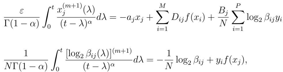Since the nature of the transfer process related to synaptic information becomes more precise using fractional differential equations, the Caputo definition for the fractional derivative is more suitable because it incorporates initial conditions and its integer order derivatives. Although there are several definitions regarding the fractional derivative of order $\alpha \geq 0$, in the time domain the general network equations describing the temporal evolution of the STM and LTM states for the $j$ -th neuron of $M$ neurons are $$ \frac{\varepsilon}{\Gamma(1 - \alpha)} \int_0^t \frac{x_j^{(m+1)}(\lambda)}{(t - \lambda)^\alpha} d\lambda = -a_j x_j + \sum_{i=1}^M D_{ij} f(x_i) + \frac{B_j}{N} \sum_{i=1}^P \log_2 \beta_{ij} y_i $$ where $\alpha$ is the Caputo's fractional order defined by $\alpha = m + \gamma$, $m \in \mathbb{Z}^+$, $0 < \gamma \leq 1$; $\Gamma(\cdot)$ is the Gamma function, $x_j$ is the current activity level (STM), $a_{j}$ is the time constant of the neuron, $B_{j}$ is the contribution of the external stimulus term, $f(x_{i})$ is the neuron's output, $y_{i}$ is the external stimulus, and $\varepsilon$ is the fast time-scale associated with the STM state. $D_{ij}$ represents a synaptic connection parameter between the $i$ -th neuron and $j$ -th neuron. According to the definition of $m_{ij}$ in (1) and unlike [1, 9, 6], the self-organizing map is implicitly modeled by a network of sources emitting input signals with a prescribed probability distribution and external stimulus $\pmb{y} \triangleq [y_i]$. By using the dynamic transform $w_j = \langle \pmb{y}, \log_2 \pmb{\beta}_j \rangle$ the model gets as follows: $$ \frac {\varepsilon}{\Gamma (1 - \alpha)} \int_ {0} ^ {t} \frac {x _ {j} ^ {(m + 1)} (\lambda)}{(t - \lambda) ^ {\alpha}} d \lambda = - a _ {j} x _ {j} + \sum_ {i = 1} ^ {M} D _ {i j} f (x _ {i}) + \frac {B _ {j}}{N} w _ {j} \tag {2} $$ $$ \frac{1}{N\Gamma(1-\alpha)}\int_{0}^{t}\frac{w_{j}^{(m+1)}(\lambda)}{(t-\lambda)^{\alpha}}d\lambda = -\frac{1}{N}w_{j} + \|\boldsymbol{y}\|^2f(x_{j}), $$ where the external stimuli are assumed to be normalized vectors of unit magnitude $\| \pmb{y} \|^2 = 1$. As each string is the realization of a stationary and ergodic stochastic process, it will be assumed a stochastic column matrix for each iteration of $\beta_{j}$, such that there exists $P\triangleq [\bar{p}_{ij}]\in \mathbb{R}^{M\times M}$, with $\sum_{i = 1}^{M}\bar{p}_{ik} = 1$ and $\beta_j^{\sigma +1} = P\beta_j^\sigma$ for $(\sigma +1)$ -th iteration. In this way, it can be noted that $\dot{\boldsymbol{\beta}}_j = \lim_{\Delta t\to 0}\frac{1}{\Delta^{k_t}} (P - I)^k\boldsymbol {\beta}_j$, such that the sum of elements in each column of $(P - I)^{k}\triangleq [p_{ij}]$ is equal to zero, i.e., $$ \beta_ {i j} ^ {(k)} = \lim _ {\Delta t \rightarrow 0} \frac{1}{\Delta^ {k} t} \sum_ {s = 1} ^ {M} p _ {i s} \beta_ {s j}, \quad \sum_ {i = 1} ^ {M} p _ {i k} = 0, \quad \text{for} \forall k. \tag{4} $$ ## III. EQUILIBRIUM AND GLOBAL ASYMPTOTIC STABILITY The existence and uniqueness of the equilibrium point are given based on flow-invariance while the global exponential stability will be based on a strict Lyapunov function for fractional-order approaches. It is well-known that the flow-invariance theory provides a qualitative viewpoint about the dynamics of a system. To begin with, it will be defined the following theorem before presenting the main results of this paper. Theorem 1. Consider the system of fractional differential equations: $$ \frac {1}{\Gamma (1 - \alpha)} \int_ {0} ^ {t} \frac {x _ {i} ^ {(m + 1)} (\lambda)}{(t - \lambda) ^ {\alpha}} d \lambda = - a _ {i} x _ {i} + \sum_ {j = 1} ^ {M} D _ {i j} f \left(x _ {j}\right) + \frac {B _ {i}}{N} w _ {i}, \tag {5} $$ $$ \frac{1}{\Gamma (1 - \alpha)} \int_ {0} ^ {t} \frac{w _ {i} ^ {(m + 1)} (\lambda)}{(t - \lambda) ^ {\alpha}} d \lambda = - \frac{1}{N} w _ {i} + f (x _ {i}),, $$ for $i = 1, \ldots, M$, where $a_i > 0$ for all $i = 1, \ldots, M$, and $f$ is locally Lipschitz and bounded, that is, there exists a constant $C > 0$ such that $-C \leq f(x) \leq C$ for all $x \in \mathbb{R}$. Then for any $\varepsilon > 0$ and for any initial condition $\{x(0), w(0)\} \in \mathbb{R}^{2M}$ there exists a $T \geq 0$ such that $$ w _ {i} (t) \in [ - C - \varepsilon , C + \varepsilon ], x _ {i} (t) \in [ - l _ {i} - \varepsilon , l _ {i} + \varepsilon ], $$ for all $i = 1,\dots,M$ with equilibrium point $e = [\bar{x}_i\quad \bar{w}_i] = [\bar{x}_i\langle \pmb {y},\log_2\bar{\beta}_i\rangle ]$ where $\forall \bar{\beta}_{ij}\in \bar{\beta}_i$ satisfies $$ \int_0^t\int_0^\lambda\frac{y_j}{\bar{\beta}_{ij}^2\ln2}\sum_{r=1}^M\sum_{q=1}^M\sum_{s=1}^M p_{is}p_{sq}p_{ir}\bar{\beta}_{qj}\bar{\beta}_{rj}\cdot d\lambda^2 = 0 $$ $$ \int_0^t\frac{y_j}{\bar{\beta}_{ij}^2\ln2}\sum_{r=1}^M\sum_{q=1}^M\sum_{s=1}^M p_{is}p_{sq}p_{ir}\bar{\beta}_{qj}\bar{\beta}_{rj} \cdot d\lambda = 0 $$ $$ S_{m}\sum_{s=1}^{M}p_{is}\bar{\beta}_{sj}y_{j}=\frac{y_{j}}{\bar{\beta}_{ij}\ln2}\sum_{r=1}^{M}\sum_{q=1}^{M}\sum_{s=1}^{M}p_{is}p_{sq}p_{ir}\bar{\beta}_{qj}\bar{\beta}_{rj}, $$ for $m = 0,1$ and 2, respectively, and $S_{m}\in \mathbb{Z}^{+}$ for all $t\geq T$ Proof. Since $f$ is Lipschitz, system (5)-(6) has local existence and uniqueness of solutions. Furthermore, since $f$ is uniformly bounded, there exist constants $K_{1},\ldots,K_{5}$ such that $$ \left| \frac {1}{\Gamma (1 - \alpha)} \int_ {0} ^ {t} \frac {x _ {i} ^ {(m + 1)} (\lambda)}{(t - \lambda) ^ {\alpha}} d \lambda \right| \leq K _ {1} + K _ {2} \| x _ {i} (t) \| + K _ {3} \| w _ {i} (t) \| $$ $$ \left| \frac{1}{\Gamma(1 - \alpha)} \int_0^t \frac{w_i^{(m+1)}(\lambda)}{(t - \lambda)^\alpha} d\lambda \right| \leq K_4 + K_5 \| w_i(t) \|, $$ thus all solutions are defined globally (for all $t \geq 0$ ). Given $\varepsilon > 0$, let $\delta_i > 0$ be defined as $$ \delta_{i} = \left\{ \begin{array}{l l} \min \left\{ \frac{a_{i}\varepsilon}{2|B_{i}|}, \varepsilon \right\} & B_{i} \neq 0 \\ \varepsilon & B_{i} = 0 \end{array} \right. $$ such that $-|B_i|\delta_i + a_i\varepsilon \geq a_i\varepsilon /2$, for all $i = 1,\ldots,M$. Then for $t\geq 0$ and for $w_i(t)\leq -C - \delta_i$ the following inequality holds: $$ \begin{array}{l} \frac {1}{\Gamma (1 - \alpha)} \int_ {0} ^ {t} \frac {w _ {i} ^ {(m + 1)} (\lambda)}{(t - \lambda) ^ {\alpha}} d \lambda \geq - \frac {1}{N} (- C - \delta_ {i}) + f (x _ {i}) = \frac {1}{N} \delta_ {i} + \\\left[ f \left(x _ {i}\right) + \frac {1}{N} C \right] \geq \delta_ {i} > 0. \tag {10} \\\end{array} $$ Similarly, for $t \geq 0$ and for $w_{i}(t) \geq C + \delta_{i}$, the following inequality holds: $$ \begin{array}{l} \frac {1}{\Gamma (1 - \alpha)} \int_ {0} ^ {t} \frac {w _ {i} ^ {(m + 1)} (\lambda)}{(t - \lambda) ^ {\alpha}} d \lambda \leq - \frac {1}{N} (C + \delta_ {i}) + f (x _ {i}) = - \frac {1}{N} \delta_ {i} + \\\left[ f \left(x _ {i}\right) - \frac {1}{N} C \right] \leq - \delta_ {i} < 0. \tag {11} \\\end{array} $$ Since $\alpha \leq 1$ then $\Gamma(1 - \alpha) > 0$ and $(t - \lambda)^{\alpha} > 0$. In that sense, from (10)-(11), both inequalities are guaranteed if and only if $w_{i}^{(m + 1)}(\lambda) > 0$ and $w_{i}^{(m + 1)}(\lambda) < 0$, respectively. By mathematical induction, it can be noted that $$ \begin{array}{l} w _ {i} ^ {(m + 1)} = \sum_ {j = 1} ^ {M} \left[ \sum_ {k = 0} ^ {m} \frac {A _ {k}}{\beta_ {i j} ^ {m + 1 - k}} (\dot {\beta} _ {i j}) ^ {m + 1 - k} y _ {j} ^ {(k)} + \frac {S _ {k}}{\beta_ {i j} ^ {m + 1 - k}} \beta_ {i j} ^ {(k + 1)} y _ {j} ^ {(m - k)} \right] \\+ \frac {d ^ {m - 2}}{d \lambda^ {m - 2}} \left. \frac {\dot {\beta} _ {i j} \ddot {\beta} _ {i j} y _ {j}}{\beta_ {i j} ^ {2} \ln 2}\right), \\\end{array} $$ where $A_{k},B_{k}\in \mathbb{Z}^{+}$. So, for $w_{i}(t)\leq -C - \delta_{i}$ and $w_{i}(t)\geq C + \delta_{i}$ $$ \begin{array}{l} \sum_ {j = 1} ^ {M} \left[ \sum_ {k = 0} ^ {m} \frac {A _ {k}}{\beta_ {i j} ^ {m + 1 - k}} (\dot {\beta} _ {i j}) ^ {m + 1 - k} y _ {j} ^ {(k)} + \frac {S _ {k}}{\beta_ {i j} ^ {m + 1 - k}} \beta_ {i j} ^ {(k + 1)} y _ {j} ^ {(m - k)} \right] > \\- \frac {d ^ {m - 2}}{d \lambda^ {m - 2}} \left. \frac {\dot {\beta} _ {i j} \ddot {\beta} _ {i j} y _ {j}}{\beta_ {i j} ^ {2} \ln 2}\right), (1 2) \\\end{array} $$ $$ \begin{array}{l} \sum_ {j = 1} ^ {M} \left[ \sum_ {k = 0} ^ {m} \frac {A _ {k}}{\beta_ {i j} ^ {m + 1 - k}} (\dot {\beta} _ {i j}) ^ {m + 1 - k} y _ {j} ^ {(k)} + \frac {S _ {k}}{\beta_ {i j} ^ {m + 1 - k}} \beta_ {i j} ^ {(k + 1)} y _ {j} ^ {(m - k)} \right] < \\\left. - \frac {d ^ {m - 2}}{d \lambda^ {m - 2}} \quad \frac {\dot {\beta} _ {i j} \ddot {\beta} _ {i j} y _ {j}}{\beta_ {i j} ^ {2} \ln 2}\right), \tag {13} \\\end{array} $$ respectively. By using (4) in (12), it can be obtained $$ \begin{array}{l} \lim _ {\Delta t \to 0} \sum_ {j = 1} ^ {M} \left[ \sum_ {k = 0} ^ {m} \frac {A _ {k}}{\Delta^ {m - k - 2} t \beta_ {i j} ^ {m + 1 - k}} \sum_ {s = 1} ^ {M} p _ {i s} \beta_ {s j} y _ {j} ^ {(k)} \right. \\\left. + \frac {S _ {k}}{\Delta^ {k - 2} t \beta_ {i j} ^ {m + 1 - k}} \sum_ {s = 1} ^ {M} p _ {i s} \beta_ {s j} y _ {j} ^ {(m - k)} \right] > \\- \lim _ {\Delta t \to 0} \frac {d ^ {m - 2}}{d \lambda^ {m - 2}} \left. \frac {y _ {j}}{\beta_ {i j} ^ {2} \ln 2} \sum_ {r = 1} ^ {M} \sum_ {q = 1} ^ {M} \sum_ {s = 1} ^ {M} p _ {i s} p _ {s q} \beta_ {q j} p _ {i r} \beta_ {r j}\right). \\\end{array} $$ For $k < m$, the evaluation of limits above yields, $$ \infty > - \frac {d ^ {m - 2}}{d \lambda^ {m - 2}} \quad \frac {y _ {j}}{\beta_ {i j} ^ {2} \ln 2} \sum_ {r = 1} ^ {M} \sum_ {q = 1} ^ {M} \sum_ {s = 1} ^ {M} p _ {i s} p _ {s q} \beta_ {q j} p _ {i r} \beta_ {r j}), \tag {14} $$ which represents an obvious condition. For $k = m$, $$ \begin{array}{l} \lim _ {\Delta t \to 0} \sum_ {j = 1} ^ {M} \left[ \frac {A _ {m} \Delta^ {2} t}{\beta_ {i j}} \sum_ {s = 1} ^ {M} p _ {i s} \beta_ {s j} y _ {j} ^ {(m)} + \frac {S _ {m}}{\Delta^ {m - 2} t \beta_ {i j}} \sum_ {s = 0} ^ {M} p _ {i s} \beta_ {s j} y _ {j} \right] \\> - \lim _ {\Delta t \to 0} \frac {d ^ {m - 2}}{d \lambda^ {m - 2}} \left. \frac {y _ {j}}{\beta_ {i j} ^ {2} \ln 2} \sum_ {r = 1} ^ {M} \sum_ {q = 1} ^ {M} \sum_ {s = 1} ^ {M} p _ {i s} p _ {s q} \beta_ {q j} p _ {i r} \beta_ {r j}\right). \\\end{array} $$ Therefore, by evaluating the limits for $m > 2$, the inequality (14) is obtained again. However, for $0 \leq m \leq 2$ (i.e., $m = 0,1$ and 2), $$ \int_ {0} ^ {t} \int_ {0} ^ {\lambda} \frac {y _ {j}}{\beta_ {i j} ^ {2} \ln 2} \sum_ {r = 1} ^ {M} \sum_ {q = 1} ^ {M} \sum_ {s = 1} ^ {M} p _ {i s} p _ {s q} p _ {i r} \beta_ {q j} \beta_ {r j}) d \lambda^ {2} > 0, \tag {15} $$ $$ \int_ {0} ^ {t} \frac {y _ {j}}{\beta_ {i j} ^ {2} \ln 2} \sum_ {r = 1} ^ {M} \sum_ {q = 1} ^ {M} \sum_ {s = 1} ^ {M} p _ {i s} p _ {s q} p _ {i r} \beta_ {q j} \beta_ {r j} \Bigg) d \lambda > 0, \tag {16} $$ $$ S _ {m} \sum_ {s = 1} ^ {M} p _ {i s} \beta_ {s j} y _ {j} < \frac {y _ {j}}{\beta_ {i j} \ln 2} \sum_ {r = 1} ^ {M} \sum_ {q = 1} ^ {M} \sum_ {s = 1} ^ {M} p _ {i s} p _ {s q} p _ {i r} \beta_ {q j} \beta_ {r j}, \tag {17} $$ respectively. Since the operator $d^{m - 2} / d\lambda^{m - 2}$ becomes an integral for $m < 2$. So, for $w_{i}(t) \leq -C - \delta_{i}$, the inequalities (15)-(17) guarantee $w^{(m + 1)} > 0$. The same treatment applies to (13), it is only to change the less than symbol in (15)-(17) by greater than symbol. Therefore, for any $i \in \{1, \ldots, M\}$ there exists a $T_{i} > 0$ such that $$ w _ {i} (t) \in [ - C - \delta_ {i}, C + \delta_ {i} ] \subseteq [ - C - \varepsilon , C + \varepsilon ], \tag {18} $$ for all $t \geq T_i$. So, the equilibrium point $\bar{w}_i = \langle \pmb{y}, \log_2 \bar{\beta}_i \rangle \in [-C - \varepsilon, C + \varepsilon]$, where $\forall \bar{\beta}_{ij} \in \bar{\beta}_i$ satisfies $$ \int_ {0} ^ {t} \int_ {0} ^ {\lambda} \frac {y _ {j}}{\bar {\beta} _ {i j} ^ {2} \ln 2} \sum_ {r = 1} ^ {M} \sum_ {q = 1} ^ {M} \sum_ {s = 1} ^ {M} p _ {i s} p _ {s q} p _ {i r} \bar {\beta} _ {q j} \bar {\beta} _ {r j} \Bigg) d \lambda^ {2} = 0, (m = 0) $$ $$ \int_ {0} ^ {t} \frac {y _ {j}}{\bar {\beta} _ {i j} ^ {2} \ln 2} \sum_ {r = 1} ^ {M} \sum_ {q = 1} ^ {M} \sum_ {s = 1} ^ {M} p _ {i s} p _ {s q} p _ {i r} \bar {\beta} _ {q j} \bar {\beta} _ {r j} \Bigg) d \lambda = 0, (m = 1) $$ $$ S _ {m} \sum_ {s = 1} ^ {M} p _ {i s} \bar {\beta} _ {s j} y _ {j} = \frac {y _ {j}}{\bar {\beta} _ {i j} \ln 2} \sum_ {r = 1} ^ {M} \sum_ {q = 1} ^ {M} \sum_ {s = 1} ^ {M} p _ {i s} p _ {s q} p _ {i r} \bar {\beta} _ {q j} \bar {\beta} _ {r j} (m = 2). $$ Defining $T_{S} = \max T_{i}$ then $w_{i}(t) \in [-C - \varepsilon, C + \varepsilon]$ holds for all $i \in \{1, \dots, M\}$ and for all $t \geq T_{S}$. Now, let $t \geq T_S$. For $x_i(t) \leq -l_i - \varepsilon$, (5) and (18) imply that $$ \begin{array}{l} \frac {1}{\Gamma (1 - \alpha)} \int_ {0} ^ {t} \frac {x _ {i} ^ {(m + 1)} (\lambda)}{(t - \lambda) ^ {\alpha}} d \lambda \geq a _ {i} (l _ {i} + \varepsilon) + \sum_ {j = 1} ^ {M} D _ {i j} f (x _ {j}) \\+ \frac {B _ {i}}{N} (- C - \delta_ {i}) \geq a _ {i} l _ {i} + a _ {i} \varepsilon - C \sum_ {j = 1} ^ {M} | D _ {i j} | + \frac {| B _ {i} |}{N}) - | B _ {i} | \delta_ {i}. \\\end{array} $$ By defining $l_{i} = \frac{C}{a_{i}}\left(\sum_{j = 1}^{M}|D_{ij}| + \frac{1}{N} |B_{i}|\right) > 0$, for $i = 1,\ldots,M$ then $$ \frac {1}{\Gamma (1 - \alpha)} \int_ {0} ^ {t} \frac {x _ {i} ^ {(m + 1)} (\lambda)}{(t - \lambda) ^ {\alpha}} d \lambda \geq - | B _ {i} | \delta_ {i} + a _ {i} \varepsilon \geq \frac {a _ {i} \varepsilon}{2} > 0. $$ Similarly, for $t \geq T_S$ and for $x_j(t) \geq l_i + \varepsilon$, (5) and (18) imply that $$ \frac {1}{\Gamma (1 - \alpha)} \int_ {0} ^ {t} \frac {x _ {i} ^ {(m + 1)} (\lambda)}{(t - \lambda) ^ {\alpha}} d \lambda \leq | B _ {i} | \delta_ {i} - a _ {i} \varepsilon \leq - \frac {a _ {i} \varepsilon}{2} < 0. $$ Since $\alpha \leq 1$ then $\Gamma(1 - \alpha) > 0$ and $(t - \lambda)^{\alpha} > 0$. In that sense, both before inequalities are guaranteed if and only if $x_{i}^{(m + 1)}(\lambda) > 0$ and $x_{i}^{(m + 1)}(\lambda) < 0$, respectively. Therefore, for any $i \in \{1, \dots, M\}$ there exists a $T_{i} > 0$ such that $$ x _ {i} (t) \in [ - l _ {i} - \varepsilon , l _ {i} + \varepsilon ] $$ for all $t \geq T_i$. Defining $T_X = \max T_i$ then $x_i(t) \in [-l_i - \varepsilon, l_i + \varepsilon]$ holds for all $i \in \{1, \dots, M\}$ and for all $t \geq T_X$. The system (5)-(6) is dissipative in $\mathbb{R}^{2M}$ and therefore, it has a compact global attractor $$ \mathcal{A} \subseteq D = \prod_{i=1}^{M} [-l_i, l_i] \times \prod_{i=1}^{M} [-C, C]. $$ It follows from the proof of Theorem 1 that the set $D$ is flow invariant under (5)-(6). In other words, $D$ is positively invariant set of (5)-(6), i.e., any solution starting in $D$ at $t = 0$ remains in $D$ for all $t \geq 0$. Furthermore, from the proof of Theorem 1 the set $H$ that contains $D$ can be contracted to a point, and since $D$ is flow-invariant with respect to (5)-(6) then by the Brower fixed point theorem implies that there exists a point $e \in D$ is an equilibrium point of (5)-(6). Theorem 2. Suppose that $f(x)$ is $\mathcal{C}^1$ with $|\dot{f}(x)| < k$ for all $x$ and $$ a _ {i} > k \quad \left. \sum_ {j = 1} ^ {M} \left| D _ {i j} \right| + \left| B _ {i} \right|\right), \quad i = 1, \dots , M, \tag {19} $$ then the equilibrium $e$ is unique. Proof. At the equilibrium point, $f(x_{i}) = \frac{1}{N} w_{i}$ from (6). Substituting these expressions in (5), it is obtained $$ 0 = - a _ {i} x _ {i} + \sum_ {j = 1} ^ {M} D _ {i j} f (x _ {j}) + B _ {i} f (x _ {i}), \quad \text{for} i = 1, \dots , M. $$ Since $a_{i} > 0$, $x_{i}$ can be expressed as $$ x _ {i} = \frac {1}{a _ {i}} \left. \sum_ {j = 1} ^ {M} D _ {i j} f (x _ {j}) + B _ {i} f (x _ {i})\right) = G _ {i} (x _ {1}, \ldots , x _ {M}). $$ The inequality (19) implies that $$ | G _ {i} (x _ {1} ^ {\prime}, \ldots , x _ {M} ^ {\prime}) - G _ {i} (x _ {1} ^ {\prime \prime}, \ldots , x _ {M} ^ {\prime \prime}) | < k | (x _ {1} ^ {\prime}, \ldots , x _ {M} ^ {\prime}) - (x _ {1} ^ {\prime \prime}, \ldots , x _ {M} ^ {\prime \prime}) |, $$ i.e., $G$ is a contracting map in $\mathbb{R}^M$. Consequently, there exists a unique fixed point of $G$. The $x_i$ -coordinates of this fixed point uniquely determine the $w_i$ -coordinates via $f(x_i) = \frac{1}{N} w_i$. Therefore, the equilibrium point is unique. Now, let $e = [\bar{x}_i \bar{w}_i] = [\bar{x}_i \langle \pmb{y}, \log_2 \bar{\beta}_i \rangle]$ be the equilibrium point of (5)-(6) and introduce the change of variables $\phi_i = x_i - \bar{x}_i$, $\varphi_i = w_i - \bar{w}_i$ which shifts $e$ to the origin. Specifically, if $f_i(\phi_i) = f(\phi_i + \bar{x}_i) - \frac{1}{N} \bar{w}_i$, then $f_i(0) = 0$ and (5)-(6) may be rewritten as $$ \frac {1}{\Gamma (1 - \alpha)} \int_ {0} ^ {t} \frac {\phi_ {i} ^ {(m + 1)} (\lambda)}{(t - \lambda) ^ {\alpha}} d \lambda = - a _ {i} \phi_ {i} + \sum_ {j = 1} ^ {M} D _ {i j} f (\phi_ {j}) + \frac {B _ {i}}{N} \varphi_ {i}, \tag {20} $$ $$ \frac {1}{\Gamma (1 - \alpha)} \int_ {0} ^ {t} \frac {\varphi_ {i} ^ {(m + 1)} (\lambda)}{(t - \lambda) ^ {\alpha}} d \lambda = - \frac {1}{N} \varphi_ {i} + f (\phi_ {i}) \mathrm {f o r} i = 1, \dots , M. \tag {21} $$ By assuming that there exists a Lyapunov function $V(t, \phi_i, \varphi_i)$ and class- $K$ functions $\gamma_i$ (for $i = 1,2,3$ ) satisfying $$ \gamma_ {1} (| \phi_ {i} |, | \varphi_ {i} |) \leq V (t, \phi_ {i}, \varphi_ {i}) \leq \gamma_ {1} (| \phi_ {i} |, | \varphi_ {i} |), $$ $$ \frac {1}{\Gamma (1 - \alpha)} \int_ {0} ^ {t} \frac {V ^ {(m + 1)} (\lambda , \phi_ {i} , \varphi_ {i}) (\lambda)}{(t - \lambda) ^ {\alpha}} d \lambda \leq - \gamma_ {3} (| \phi_ {i} |, | \varphi_ {i} |), $$ then the system (20)-(21) becomes asymptotically stable at equilibrium point $e$ [7]. Lemma 1. \[see [7]\] Let $r(t) \in \mathbb{R}$ be a continuous and derivable function. Then, for any time $t \geq t_0$ $$ \frac {1}{2 \Gamma (1 - \alpha)} \int_ {0} ^ {t} \frac {[ r ^ {2} (\lambda) ] ^ {(m + 1)}}{(t - \lambda) ^ {\alpha}} d \lambda \leq \frac {r (t)}{2 \Gamma (1 - \alpha)} \int_ {0} ^ {t} \frac {r (\lambda) ^ {(m + 1)} (\lambda)}{(t - \lambda) ^ {\alpha}} d \lambda . 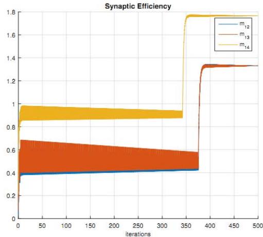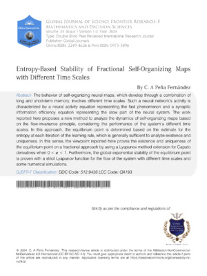$$   Figure 1: Evolution of synaptic efficiency $m_{ij}$ (for $i = 1, j = 2,3,4$ ) toward equilibrium point (1.336, 1.336, 1.768) after $N = 500$ iterations when each neuron receives an external stimulus based on neighborhood's winner.  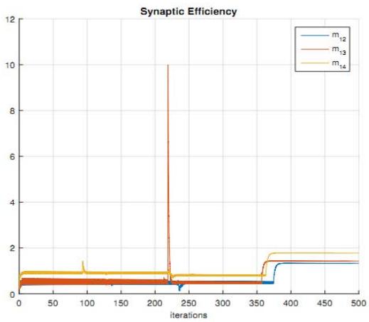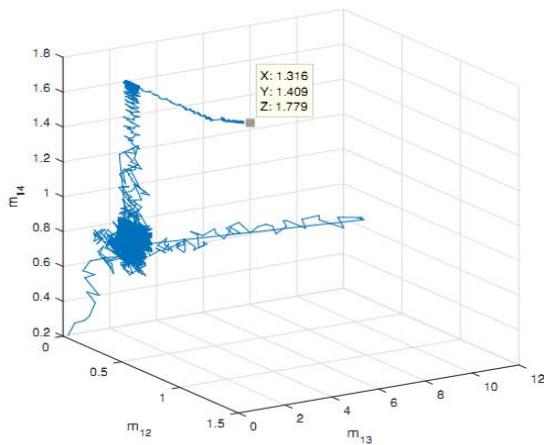 Figure 2: Evolution of synaptic efficiency $m_{ij}$ (for $i = 1, j = 2,3,4$ ) toward equilibrium point (1.316, 1.409, 1.779) after $N = 500$ iterations when each neuron updates its weights without external stimulus. Theorem 3. Suppose that $f(x)$ is $\mathcal{C}^1$ with $|\dot{f}(x)| \leq k$ for all $x$ and $a_i > 0$. If $$ \max _ {i} \left\{\frac{1}{2} \left(\frac{\left| B _ {i} \right|}{a _ {i}} + k\right) + \sum_ {j = 1} ^ {M} \frac{1}{2} k \left(\frac{\left| D _ {i j} \right|}{a _ {i}} + \frac{\left| D _ {j i} \right|}{a _ {j}}\right) \right\} < 1 $$ then $e$ is a global attractor for the system (20)-(21). Moreover, all solutions of (20)-(21) converge to $e$ exponentially fast as $t \to \infty$. Proof. The global convergence will be proved by using a Lyapunov function for (20)-(21). Let $$ V (\phi_ {i}, \varphi_ {i}) = \frac {1}{2} \sum_ {i = 1} ^ {M} \left(\frac {\phi_ {i} ^ {2}}{a _ {i}} + \varphi_ {i} ^ {2}\right), $$ then the fractional derivative for $V(\phi_i,\varphi_i)$ is defined by $$ \begin{array}{l} \frac {1}{\Gamma (1 - \alpha)} \int_ {0} ^ {t} \frac {V ^ {(m + 1)} (\phi_ {i} , \varphi_ {i})}{(t - \lambda) ^ {\xi}} d \lambda = \\\frac {1}{2 \Gamma (1 - \alpha)} \sum_ {i = 1} ^ {M} \left(\frac {1}{a _ {i}} \int_ {0} ^ {t} \frac {[ \phi_ {i} ^ {2} (\lambda) ] ^ {(m + 1)}}{(t - \lambda) ^ {\alpha}} d \lambda + \int_ {0} ^ {t} \frac {[ \varphi_ {i} ^ {2} (\lambda) ] ^ {(m + 1)}}{(t - \lambda) ^ {\alpha}} d \lambda\right), \\\end{array} $$ and by using the Lemma 1 together with (20)-(21) yields $$ \begin{array}{l} \frac {1}{\Gamma (1 - \alpha)} \int_ {0} ^ {t} \frac {V ^ {(m + 1)} \left(\phi_ {i} , \varphi_ {i}\right)}{(t - \lambda) ^ {\alpha}} d \lambda \leq - \sum_ {i = 1} ^ {M} \left(\phi_ {i} ^ {2} + \varphi_ {i} ^ {2}\right) \tag {23} \\+ \sum_ {i = 1} ^ {M} \sum_ {j = 1} ^ {M} D _ {i j} \frac {\phi_ {i}}{a _ {i}} f _ {j} (\phi_ {j}) + \sum_ {i = 1} ^ {M} \varphi_ {i} \left(\frac {\phi_ {i}}{a _ {i}} B _ {i} + f _ {i} (\phi_ {i})\right). \\\end{array} $$ Since $f_{i}(0) = 0$ and $|\dot{f}_i(x)| = |\dot{f} (x + \bar{x}_i)| < k$, it is possible to have $|f_{i}(\phi_{i})| < k|\phi_{i}|$. Consequently, with this last fact and the Minkowski inequality, (23) can be replaced by the inequality $$ \begin{array}{l} \frac {1}{\Gamma (1 - \alpha)} \int_ {0} ^ {t} \frac {V ^ {(m + 1)} (\phi_ {i} , \varphi_ {i})}{(t - \lambda) ^ {\alpha}} d \lambda < - \sum_ {i = 1} ^ {M} \left(\phi_ {i} ^ {2} + \varphi_ {i} ^ {2}\right) \\+ \sum_ {i = 1} ^ {M} \sum_ {j = 1} ^ {M} | D _ {i j} | k \frac {1}{a _ {i}} | \phi_ {i} | | \phi_ {j} | + \sum_ {i = 1} ^ {M} \left(\frac {| B _ {i} |}{a _ {i}} + k\right) | \varphi_ {i} | | \phi_ {i} |. \\\end{array} $$ The right-hand side of this inequality is given by the quadratic form with the matrix $-Q$ where $Q$ has the following structure: $$ Q = \left[ \begin{array}{c c c c c} 1 - \frac {1}{2} k \left(\frac {| D _ {1 1} |}{a _ {1}} + \frac {| D _ {1 1} |}{a _ {1}}\right) & - \frac {1}{2} \left(\frac {| B _ {1} |}{a _ {1}} + k\right) & - \frac {1}{2} k \left(\frac {| D _ {1 2} |}{a _ {1}} + \frac {| D _ {2 1} |}{a _ {2}}\right) & 0 & \dots \\- \frac {1}{2} \left(\frac {| B _ {1} |}{a _ {1}} + k\right) & 1 & 0 & 0 & \dots \\- \frac {1}{2} k \left(\frac {| D _ {2 1} |}{a _ {2}} + \frac {| D _ {1 2} |}{a _ {1}}\right) & 0 & 1 - \frac {1}{2} k \left(\frac {| D _ {2 2} |}{a _ {2}} + \frac {| D _ {2 2} |}{a _ {2}}\right) & - \frac {1}{2} \left(\frac {| B _ {2} |}{a _ {2}} + k\right) & \dots \\0 & 0 & - \frac {1}{2} \left(\frac {| B _ {2} |}{a _ {2}} + k\right) & 1 & \dots \\\vdots & \vdots & \vdots & \vdots & \ddots . \\\vdots & \vdots & \vdots & \vdots & \end{array} \right]. $$ According to Gerschgorin's theorem applied to $-Q$, there are $M$ disks centered at $z = -1$ (in $\mathbb{C}$ -plane) with radius $\frac{1}{2}\left(\frac{|B_i|}{a_i} + k\right)$. In the same way, there are $M$ disks centered at $z = \frac{1}{2}k\left(\frac{|D_{ii}|}{a_i} + \frac{|D_{ii}|}{a_i}\right) - 1$ and radius $\frac{1}{2}\left(\frac{|B_i|}{a_i} + k\right) + \sum_{j=1}^{M} \frac{1}{2}k\left(\frac{|D_{ij}|}{a_i} + \frac{|D_{ji}|}{a_j}\right)$. If condition (22) is valid then all eigenvalues $q$ of $-Q$ satisfy $q < 1$ or $$ \frac{1}{2}k\left(\frac{|D_{ii}|}{a_i} + \frac{|D_{ii}|}{a_i}\right) - 2 < q < \frac{1}{2}k\left(\frac{|D_{ii}|}{a_i} + \frac{|D_{ii}|}{a_i}\right). $$ Since $\frac{1}{2} k\left(\frac{|D_{ii}|}{a_i} + \frac{|D_{ii}|}{a_i}\right) > 0$ for $\forall i$ then $-Q$ is positive definite and $Q$ is negative definite. Therefore, let $\xi > 0$ the smallest eigenvalue of $-Q$ such that $$ \frac {1}{\Gamma (1 - \alpha)} \int_ {0} ^ {t} \frac {V ^ {(m + 1)} (\phi_ {i} , \varphi_ {i})}{(t - \lambda) ^ {\alpha}} d \lambda < - \xi \sum_ {i = 1} ^ {M} \left(\phi_ {i} ^ {2} + \varphi_ {i} ^ {2}\right), $$ and consequently, $V$ is a strict Lyapunov function for (20)-(21). Moreover, $2V \leq \sum_{i=1}^{M} (\phi_i^2 + \varphi_i^2)$ thus $$ \frac {1}{\Gamma (1 - \alpha)} \int_ {0} ^ {t} \frac {V ^ {(m + 1)} (\phi_ {i} , \varphi_ {i})}{(t - \lambda) ^ {\alpha}} d \lambda < - 2 \xi V. $$ This result implies that $V$ converges to zero exponentially fast, and the solutions $(\phi_i,\varphi_i)$ converge to the origin also exponentially fast, i.e., solutions $(x,w)$ in system (5)-(6) converges exponentially fast to equilibrium $e = [\bar{x}\langle \pmb {y},\log_2\bar{\pmb{\beta}}_1\rangle \dots \langle \pmb {y},\log_2\bar{\pmb{\beta}}_M\rangle ]$ 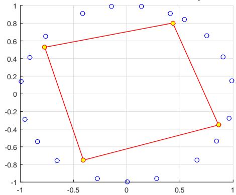 Final iteration WITHOUT external stimulus, $||y_i|| = 0$ 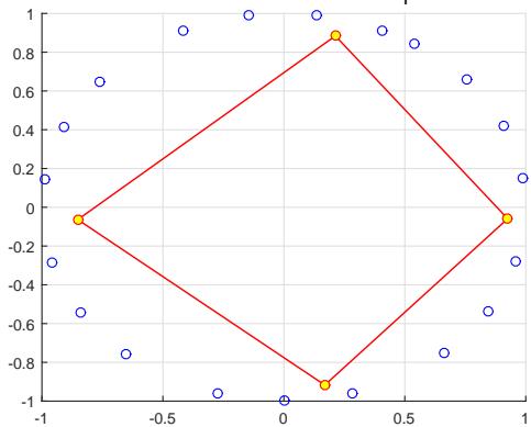 Final iteration WITH external stimulus, $\| y_i \| \neq 0$ Figure 3: Comparing last iteration ( $N = 500$ iterations) related to SOM for circle pattern composed by 20 points. ## IV. ACCESSING NUMERICAL SIMULATIONS To validate the proposed model, a self-organizing map with four neurons $(M = 4)$ is utilized in the following example. The aim is to find the best updating of synaptic weights to adjust a circle shape that consists of 20 patterns and has a radius of 0.5. This will be achieved using unsupervised Hebb's learning rule with $N = 500$ and a learning rate of 0.05. Let's assume that each neuron in a neural network has an activation value of $a_{j} = 0.5$. Two parameters, $D_{ij}$ and $B_{j}$, were set randomly for each neuron within the range of 0 to 1. Additionally, $\alpha$ was set to 0.5, $m$ to 0, and $\varepsilon$ to $10^{-4}$. To analyze the behavior of the equilibrium point in this model, the algorithm ran for 500 iterations and observed how the equilibrium point behaves. Theorem 1 was used to determine the stability of this point. Our results show that the model is locally stable, which means that it is capable of reaching an equilibrium point and maintaining its over time. In order to illustrate this point, Fig. 1 illustrates the equilibrium point (1.336, 1.336, 1.768) after 500 iterations with no external stimulus, meaning that $\| y_{i} \| = 0$ and $m_{ij} = \frac{1}{N} \log_2 \beta_{ij}$ for $i = 1$ and $j = 2,3,4$. This means that all sequences $(\sigma_{1}, \ldots, \sigma_{500})$ for events set $X = \emptyset$ between two neurons have a probability of one, and the entropy $H_{i}$ $(i = 1,2,3,4)$ approaches zero, which is the ideal situation. The following text describes the behavior of neurons when an external stimulus is applied. So, let's compare two figures - Fig. 1 and Fig. 2. The former shows the neurons' behavior when no external stimuli are applied, while the latter shows their behavior when stimuli are applied. The amplitude of the impulses generated by the stimuli is set at 0.001, and the stimuli are defined by one impulse over the threshold. The sequences $(\sigma_{1},\ldots,\sigma_{500})$ associated with each neuron are considered as a result of updating synaptic weights according to the training rule at each iteration. In a neural network, when a neuron is declared a winner and its weights are updated, the weights of the neighboring neuron also need to be updated. Therefore, for each iteration in the process, every neuron must have a term called $\sigma_{i}$ in its sequence. This term should be equal to one when the neuron is updated and zero when it doesn't receive any updates in its weights. Figure 3 illustrates that neurons form a circular pattern consisting of 20 points; however, the final position of neurons changes due to external stimuli during the last iteration. For both cases in Figures 1 and 2, the equilibrium point $(\bar{\beta}_{12},\bar{\beta}_{13},\bar{\beta}_{14})$ is represented by (1.336, 1.336, 1.768) and (1.316, 1.409, 1.779). By assuming only the synaptic efficiencies $m_{12}, m_{13}, m_{14}$, condition (7) becomes the following three conditions: $$ \frac{p_{11}}{\ln 2} \sum_{s=1}^{M} p_{1s} p_{s1} \int_{0}^{t} \int_{0}^{\lambda} y_{4} \cdot d\lambda^{2} = 0, $$ $$ \frac {p _ {1 1}}{\ln 2} \sum_ {s = 1} ^ {M} p _ {1 s} p _ {s 1} \int_ {0} ^ {t} \int_ {0} ^ {\lambda} y _ {3} \cdot d \lambda^ {2} = 0, $$ $$ \frac{p _ {1 1}}{\ln 2} \sum_ {s = 1} ^ {M} p _ {1 s} p _ {s 1} \int_ {0} ^ {t} \int_ {0} ^ {\lambda} y _ {2} \cdot d \lambda^ {2} = 0, $$  i.e., the external stimulus has no contribution in the final stage of training for neurons connected to neuron 1. On another side, it can be observed from Figs. 1 and 2 that the evolution of $m_{1j}$ ( $j = 2,3,4$ ) ensures the condition $SIE_1 > SIE_j$, more specifically, $$ \begin{array}{l} H _ {i} (\sigma_ {1}, \ldots , \sigma_ {5 0 0} | S _ {i n}) - H _ {j} (\sigma_ {1}, \ldots , \sigma_ {5 0 0} | S _ {i n}) \\> H _ {i} (\sigma_ {1}, \ldots , \sigma_ {5 0 0}) - H _ {j} (\sigma_ {1}, \ldots , \sigma_ {5 0 0}). \\\end{array} $$ This result indicates that the motion of neurons without an external stimulus is less disorganized than the motion of neurons with an external stimulus, as expected. ## V. FINAL REMARKS The following paper establishes the global exponential stability of SOMs. To this end, this proposal has used fractional order derivatives to describe cognitive cortical maps that result from self-organization, with both LTM and STM approaches. It applied McMillan-Shannon's approach to fractional competitive differential equations, which helps to understand the entropy behavior of SOM in response to external stimuli. The proposal not only proves the existence and uniqueness of the equilibrium point but also shows how fractional order derivative operators can improve our understanding of entropy associated with synaptic efficiency. Synaptic efficiency was modeled by using sequences of updating impulses at each iteration, all of them as a result of applying external stimuli, not only for the winner neuron but also for neighbor neurons. In this way, the concept of conditional entropy plays an important role in the proposal as it shows that it must be greater than entropy to ensure convergence to the equilibrium point. In future studies, it is hoped to investigate the correlation between the development of information transfer and the division of fast dynamics into distinct time scales. This will involve integrating the Dynamic Confined Space of Velocities criterion (DCSV) [14] into restricted self-organizing maps, which are extensively utilized to address constrained multi-objective optimization issues (CMOPs) [15]. ### ACKNOWLEDGMENTS The author would like to thank IFBA for the research funding provided through Announcements n.01/2021-PIS/IFBA, n.01/2023-DPGI/IFBA and Research Procedure SEI n.23279.005450/2022-48

Generating HTML Viewer...

References

18 Cites in Article
A Meyer-Baese,S Pilyugin,Y Chen (2003). Global exponential stability of competitive neural networks with different time scales.
(null). Figure 1. Synaptic drive and spiking rate of neurons in a recurrent network can learn complex patterns..
S.-I Amari (1982). Competitive and Cooperative Aspects in Dynamics of Neural Excitation and Self-Organization.
V Final Remarks Ref.
C Peña Fernández (2023). An Ergodic Selection Method for Kinematic Configurations in Autonomous, Flexible Mobile Systems.
Michael Lemmon,B Vijaya Kumar (1989). Emulating the dynamics for a class of laterally inhibited neural networks.
Michael London,Adi Schreibman,Michael Häusser,Matthew Larkum,Idan Segev (2002). The information efficacy of a synapse.
D Willshaw,V Malsburg (1976). How patterned neural connections can be setup by self-organization.
S Najafian,E Koch,K Teh,J Jin,H Rahimi-Nasrabadi,Q Zaidi,J Kremkow,J.-M Alonso (2022). A theory of cortical map formation in the visual brain.
Norelys Aguila-Camacho,Manuel Duarte-Mermoud,Javier Gallegos (2014). Lyapunov functions for fractional order systems.
Shuo Zhang,Yongguang Yu,Junzhi Yu (2017). LMI Conditions for Global Stability of Fractional-Order Neural Networks.
Jia Jia,Xia Huang,Yuxia Li,Jinde Cao,Ahmed Alsaedi (2020). Global Stabilization of Fractional-Order Memristor-Based Neural Networks With Time Delay.
Ailong Wu,Zhigang Zeng (2017). Global Mittag–Leffler Stabilization of Fractional-Order Memristive Neural Networks.
Jiejie Chen,Zhigang Zeng,Ping Jiang (2014). Global Mittag-Leffler stability and synchronization of memristor-based fractional-order neural networks.
Thomas Cover,Joy Thomas (2006). Elements of Information Theory.
George Saridis (2001). Entropy in Control Engineering.
C Peña Fern´ández (2023). An Ergodic Selection Method for Kinematic Configurations in Autonomous, Flexible Mobile Systems.
Chao He,Ming Li,Congxuan Zhang,Hao Chen,Peilong Zhong,Zhengxiu Li,Junhua Li (2022). A self-organizing map approach for constrained multi-objective optimization problems.
No ethics committee approval was required for this article type.
Data Availability
Not applicable for this article.
How to Cite This Article
C.A Pena Fernandez. 2026. \u201cEntropy-based Stability of Fractional Self-Organizing Maps with Different Time Scales\u201d. Global Journal of Science Frontier Research - F: Mathematics & Decision GJSFR-F Volume 24 (GJSFR Volume 24 Issue F1): .
Explore published articles in an immersive Augmented Reality environment. Our platform converts research papers into interactive 3D books, allowing readers to view and interact with content using AR and VR compatible devices.
Your published article is automatically converted into a realistic 3D book. Flip through pages and read research papers in a more engaging and interactive format.
The behavior of self-organizing neural maps, which develop through a combination of long and short-term memory, involves different time scales. Such a neural network’s activity is characterized by a neural activity equation representing the fast phenomenon and a synaptic information efficiency equation representing the slow part of the neural system. The work reported here proposes a new method to analyze the dynamics of self-organizing maps based on the flow-invariance principle, considering the performance of the system’s different time scales. In this approach, the equilibrium point is determined based on the estimate for the entropy at each iteration of the learning rule, which is generally sufficient to analyze existence and uniqueness. In this sense, the viewpoint reported here proves the existence and uniqueness of the equilibrium point on a fractional approach by using a Lyapunov method extension for Caputo derivatives when 0 < 𝛼𝛼 < 1. Furthermore, the global exponential stability of the equilibrium point is proven with a strict Lyapunov function for the flow of the system with different time scales and some numerical simulations.
Our website is actively being updated, and changes may occur frequently. Please clear your browser cache if needed. For feedback or error reporting, please email [email protected]
Thank you for connecting with us. We will respond to you shortly.