


I. INTRODUCTION
Consider the problem of estimating the proportion of true null hypotheses in a collection of m tests, given the observed p-values for the collection of m tests. This problem has attracted a lot of attentions in statistical literatures, attributing to its important role in dealing with multiple testing procedures, since the nominal paper Storey (2002). It has naturally arisen in assessing or controlling an overall false rejection rate, i.e., the false discovery rate (FDR) proposed by Benjamini and Hochberg (1995) in multiple null hypothesis testing problems and multiple comparisons. Benjamini and Hochberg proved that if are independent with continuous distributions, the popular Sime's multiple testing procedure (Sime 1986), where a null hypothesis is rejected whenever the observed p-value is less than , results in an FDR controlled by . Therefore, a reliable estimate is essential to control the FDR in the Sime's multiple testing procedure and improve its testing power. On the other hand, the proportion is a quantity of interest in its own right. For example, researchers may wish to estimate the proportion of genes that are not differentially expressed in DNA microarray experiments (Parker et. al. 1988).
Store (2002) proposed to approach the estimating problem from a Bayesian point of view by treating as a random sample of size from a mixture distribution of a uniform distribution and a non-uniform distribution with mixing proportion .
f(x|\pi_0,h) = \pi_0 + (1 - \pi_0)h(x),\0 \leq x \leq 1.By Storey's approach, the observed -values are considered to be a random sample of size from . As a consequence, the mixing proportion in the mixture model (1) represents the proportion of true-null -value subpopulation and an estimate for based on a random sample from (1) thus yields an estimate for the proportion of true null hypotheses among the null hypotheses in the multiple testing problem.
The first well-studied estimator for was proposed by Storey (2002) as follows:
where is an appropriately chosen value close to 1 and is the total number of the p-values greater than . This estimator is motivated by the fact that false-null p-values are typically small so that with close to 1, is close to the expected proportion of true-null p-values falling into . Since the proportion of the p-values falling into is a mixture of and with mixing proportions , is obtained mathematically by simply setting the proportion of false-null p-values falling into to be zero, i.e., . As a consequence, tends to overestimate , as is typically positive. The biasedness can be too great to be acceptable when belongs to the lower part of [0, 1]. Storey (2002) proposed a bootstrap procedure to choose that minimizes an upper bound of the mean square error of the resulting positive FDR estimator where . See more discussion and some other work on how to select , see Storey, Taylor and Siegmund (2004), and Nettleton, Hwang, Caldo and Wise (2006).
Since the publication of Storey (2002), the mixture model approach described above has been adopted widely and many other estimators have been proposed. They include: Langaas, Lindqvist and Ferkingstad (2005)'s by a histogram approach, Wu, Guan and Zhao (2006)'s polynomial-type estimator, Jiang and Doerge (2008)'s estimator averaging over different -values with Storey (2002)'s estimator, Zhao, Wu, Zhang and Chen (2012)'s estimator in exponential mixture model, Cheng, Gao and Tong (2015)'s estimator with reduction of estimating bias and standard deviation. For more references and discussion, see Cheng, Gao and Tong (2015), and Tong, Feng, Hilton and Zhao (2013) that deals with possibly dependent p-values. Nevertheless, when these estimators are intended to improve some aspects of Storey's estimator, the biasedness remains significant even with m as large as 2,000, especially when is not close to 1. Motivated by the histogram approach (see Mosig et al. 2001 and Nettleton et al. 2006), a new estimator is proposed in this paper via a likelihood approach with h being approximated by a modified histogram pdf. Akaike information criterion is used to select the number of categories in histogram construction. Simulation study demonstrates that the new estimator significantly improves popularly cited existing methods such as Storey (2002), Langaas, Lindqvist and Ferkingstad Langaas (2005), Jiang and Doerge (2008) and Nettleton et al.(2006).
The paper is organized as follows. The new method along with discussion of computing issues is presented in Section 2. Simulation results are reported in Section 3. A real-life example is given in Section 4.
II. METHOD
Let be a random sample of size from the pdf defined in (1). We propose to be estimated by the MLE when is subject to a histogram-type approximation. We shall proceed with a study on the identification problem in the mixture model.
a) Identification
Let be the parameter space consisting of all 's with and being a probability density function on and continuous in a neighborhood of 1 with , where
For convenience and confirmation, when a pdf is used as a parameter throughout the paper, we should refer to the probability distribution, say the CDF specified by the pdf.
Lemma 1 The distribution in the model (1) is identifiable in .
Proof. Let two parameter sets and in define the same distribution, i.e., for any ,
where is the CDF of . Since and are continuous in a common neighborhood of 1, (2) implies that for any x in a neighborhood of 1,
So because . This in turn implies in (2) because and . The lemma is proved.
Remarks.
(a) First of all, note the simple fact that implies that is non-uniform. Of course, identification of the parameter of interest requires that is non-uniform.
(b) When , is un-identifiable in .
(c) The assumption that is continuous in a neighborhood of 1 with is critical. Without it, the lemma can fail. For a counterexample, let and , and and . We have
and for any in
and
That is, for all in , but and .
b) A
Motivated by the histogram approach (see Mosig et al. (2001), a histogram approximation to the alternative pdf is proposed as follows. Let k > 2 be an integer. Define
Notes
where satisfying . The linear modification over the right most subinterval warrants so that is identifiable in and . As Storey(2002) and Tong et al. (2013) remarked, the false-null p-values that follow the distribution h are typically small. In other words it is often the case in application that the alternative pdf h is highly skewed to the right. Therefore, with the linear modification on the rightmost subinterval , the effect on the accuracy of the estimate for Storey (2002), Jiang and Doerge (2008) and some other methods assume that h is zero in a neighborhood of 1.
c) The new estimator with fixed k
Suppose that k > 2 is specific for now (a selection procedure will be described later). When h is approximated by or restricted to , with a random sample , the log-likelihood of the parameter of interest and the new nuisance parameter q becomes
where is the indicator whether falls into the j-th category of the histogram with k bins or not, i.e.,
for
Let be the MLE of with the log-likelihood function (3), subject to and , such that . This defines the new estimator for with specified k. A direct application of the standard theory of MLE yields the following theorem and hence a theory of consistency of the new estimator.
Theorem 1 For any and , let
Notes for . Put and . Then converges to in distribution, as , where
d) Computation of
Maximizing the nonlinear log-likelihood function (3) can be complicating. However, the EM algorithm can be used to obtain an approximation to the MLE easily. To do so, introduce a latent Bernoulli variable indicating the component-ship of the -value in the finite mixture distribution. That is, let be a binary random variable with and , and let a random variable follow the distribution as follows. Given , follows the uniform distribution on and given , . It is clear that follows the mixture distribution . Thus can be viewed as the incomplete data of a random sample from with missing values .
Note that with the complete data , the likelihood function of is
where 's are defined in (4), and the log-likelihood function is thus
where , and .
The EM algorithm can be easily implemented as follows. Let be the current approximations to the MLE with the log-likelihood function l given in (3). The next approximation is given by the EM algorithm in two steps, the so-called E-step and M-step.
E-Step: Compute the conditional expectation of the log-likelihood function
Note
Notes
We have
M-Step: In the M-step, is maximized to yield the next approximation and . Setting , we immediately have
By Lemma 2 in Appendix,
The formulas in the EM algorithm above are similar to those developed by Oluyemi (2016) and Oluyemi and Chen (2016) where there are some algebraic errors.
where
e) Selection of k via AIC
In this subsection, we discuss about selection of k. As a histogram-type approximation to , the value of k can reveal different features of the data. Since k is the number of categories of the histogram fitting h, a larger value of k does a better fitting job and hence is expected to result in a more accurate estimate of . However, a larger value of k causes a greater standard error in estimating because there are more nuisance parameters to handle. As the estimate is based on the likelihood function, the Akaike information criterion (AIC) can be a nature choice of criteria for selection of an appropriate value of k. Let be the maximum value of the log-likelihood function l defined in (3), i.e., . Noting that we have total of k - 1 free parameters in computing , the AIC selection of k is to choose such that is maximized, i.e.,
The final estimate for is .
III. SIMULATION STUDY
Simulation studies are conducted with the p-values based on one-sided z-test in finite normal mixture models to evaluate the performance of the new estimator and compare it with some existing method. Specifically, consider the finite normal model with five griding values of : 0.2, 0.35, 0.50, 0.65 and 0.8. The p-value is computed by . Four sample sizes, m=500, 1000, 1500 and 2000 are considered. With each combination, 2000 Monte Care trials are used.
In the simulation studies, the EM algorithm is used to approximate the MLE's and a linear algorithm is used to search for the AIC selection .
Four existing estimators popularly cited in the literature are considered for purpose of comparison. They are Storey's estimator with bootstrap method , the convex density estimator by Langaas, Lindqvist and Ferkingstad (2005), the averaging Storey estimator by Jiang and Doerge (2008) and the histogram estimator by Nettleton, Hwang, Caldo, and Wise (2006). The package cp4p is used for computations of these estimates; all the computations are done with default settings of the package.
Simulation results are reported in Table 1. The following findings from the simulation studies are immediate:
The new estimatorperforms very well. A clear converging pattern is demonstrated in each simulation model, asincreases. The convergence with lower values ofis faster than with higher values.
The new estimator performs substantially better than all other four existing estimators. It is noted that the Storey's performs somewhat better than the other three existing estimators in general and its best performance is on the higher values of as expected. See Storey (2002).
IV. REAL DATA ANALYSIS
In this section, we apply the new estimate method to the real life data from Hedenfalk et al. (2001) where 3226 genes were studied with BRECA1 arrays and BRCA2 arrays. The example is to test with each gene the null hypothesis that there is no differential gene expression between BRCA1-mutation-positive tumors and BRCA2-mutation-positive tumors by using a two-sample t-statistic. It was also analyzed by Storey and Tibshirani (2003). Following their instructions, we were able to download the p-values from http://www.genomine.org/qvalue/results.txt. Removing missing values left with m=2752 p-values.
| m | ||||||
| 500 | 0.20 | 0.194(0.101) | 0.339(0.059) | 0.324(0.061) | 0.357(0.068) | 0.378(0.593) |
| 500 | 0.35 | 0.327(0.116) | 0.454(0.066) | 0.569(0.066) | 0.488(0.067) | 0.507(0.096) |
| 500 | 0.50 | 0.457(0.130) | 0.586(0.067) | 0.583(0.065) | 0.618(0.066) | 0.644(0.086) |
| 500 | 0.65 | 0.605(0.123) | 0.710(0.069) | 0.712(0.064) | 0.746(0.060) | 0.773(0.068) |
| 500 | 0.80 | 0.749(0.113) | 0.826(0.066) | 0.834(0.059) | 0.864(0.052) | 0.885(0.051) |
| 1000 | 0.20 | 0.202(0.082) | 0.328(0.044) | 0.308(0.047) | 0.322(0.057) | 0.314(0.085) |
| 1000 | 0.35 | 0.336(0.095) | 0.455(0.049) | 0.445(0.051) | 0.462(0.060) | 0.468(0.086) |
| 1000 | 0.50 | 0.480(0.093) | 0.583(0.052) | 0.578(0.050) | 0.599(0.055) | 0.615(0.074) |
| 1000 | 0.65 | 0.624(0.089) | 0.701(0.052) | 0.707(0.049) | 0.729(0.052) | 0.750(0.065) |
| 1000 | 0.80 | 0.777(0.084) | 0.829(0.050) | 0.834(0.044) | 0.886(0.041) | 0.875(0.042) |
| 1500 | 0.20 | 0.206(0.072) | 0.292(0.042) | 0.291(0.040) | 0.298(0.051) | 0.294(0.071) |
| 1500 | 0.35 | 0.348(0.079) | 0.423(0.049) | 0.433(0.044) | 0.440(0.056) | 0.449(0.074) |
| 1500 | 0.50 | 0.480(0.081) | 0.553(0.053) | 0.569(0.043) | 0.581(0.054) | 0.579(0.070) |
| 1500 | 0.65 | 0.636(0.075) | 0.684(0.055) | 0.703(0.043) | 0.721(0.048) | 0.741(0.055) |
| 1500 | 0.80 | 0.788(0.068) | 0.801(0.050) | 0.829(0.040) | 0.848(0.039) | 0.870(0.042) |
| 2000 | 0.20 | 0.206(0.066) | 0.295(0.038) | 0.290(0.035) | 0.292(0.045) | 0.284(0.062) |
| 2000 | 0.35 | 0.348(0.071) | 0.425(0.042) | 0.434(0.037) | 0.435(0.050) | 0.436(0.067) |
| 2000 | 0.50 | 0.496(0.065) | 0.556(0.047) | 0.571(0.038) | 0.579(0.051) | 0.585(0.065) |
| 2000 | 0.65 | 0.636(0.071) | 0.683(0.050) | 0.700(0.038) | 0.713(0.047) | 0.731(0.056) |
| 2000 | 0.80 | 0.798(0.056) | 0.812(0.047) | 0.831(0.035) | 0.847(0.035) | 0.865(0.038) |
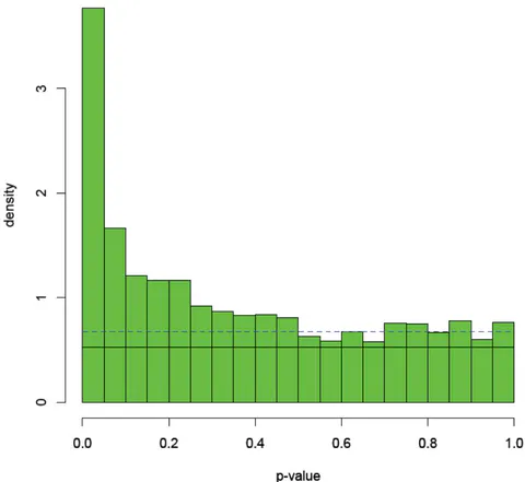
The estimates for the proportion of true null hypotheses by the new estimator and the other four existing estimators are listed in Table 2. The AIC selection of k for the new estimator is . In Figure 1 for the histogram of the 2752 available p-values with data in Hedenfalk et al. (2001), the solid horizontal line would be the expected bottom of the graph of the density function of the p-value under assumption if the real value of were equal to the estimate (0.523), whereas the dash line would indicate the expected bottom of the graph of the density function if the real value of were equal to the histogram estimate . It is evident from Figure 1 that the existing estimators overestimates .
| 0.523 | 0.689 | 0.682 | 0.704 | 0.677 |
Appendix: Computation for the estimate of q
In M-step of the EM iteration algorithm, we compute the update for the estimate of q based on the following result.
Lemma 2 Let , where are constant and such that
Notes
Then the maximum of g is attained at where
PROOF. Let
We have and
Setting all the partial derivatives to be zero yields
Adding all the equations above gives the solution of and so the solutions for . The lemma is proved.