## I. INTRODUCTION TO THE PERIODIC NAVIER STOKES EQUATIONS The Navier-Stokes equations are useful because they describe the physics of many phenomena of scientific and engineering interest. They may be used to model the weather, ocean currents, pipe flows and heat exchangers and air flow around a wing. The Navier-Stokes equations, in their full and simplified forms, help with the design of aircraft and automobiles, hemodynamics, the design of power stations, the analysis of pollution and fuel emissions and many other things. In 1845, Stokes had derived the equation of motion of a viscous flow by adding Newtonian viscous terms and finalized the Navier-Stokes equations, which have now been used for almost two centuries. There are only a few studies to find how to understand the physical meaning of the viscous terms in NS equations. As is well known, Stokes had three assumptions: 1. The force on fluids is the stationary pressure when the flow is stationary. 2. Fluid viscosity is isotropic. 3. Fluid flow follows Newton's law that fluid stress and strain have linear relations. These assumptions lead to the NSE. In [1], since the regular NS equations are quite demanding in computational time and resources the vorticity part is considered as the only source of fluid stress for the purpose of computation cost reduction. In fact, fluid shear stress is contributed by both strain and vorticity. In mathematics, the computation of stress can be performed by strain only, vorticity only, or both. The computational results are exactly the same. The NSE equation adopts strain, which is symmetric and stress based on Stokes's assumption. In [1], a new governing equation which is based on a new assumption that accepts that fluid stress has a linear relation with vorticity, which is anti-symmetric. According to the mathematical analysis, the new governing equation is identical to NS equations in numerical analysis, but in a physical sense, the new governing equation is just the opposite to NSEs as it assumes that fluid stress is proportional to vorticity, where both are anti-symmetric, but not strain, contrary to Stokes's assumption and the current NSE. Although both NSEs and the new governing equation in [1] lead to the same computational results for laminar flow, the new governing equation has several advantages: 1. The vorticity tensor is anti-symmetric, which has three elements, but NSEs use the strain tensor, which has six elements. It is shown that the computational cost is reduced to half for the viscous term. 2. The anti-symmetric matrix is independent of the coordinate system change or Galilean invariant, but the symmetric matrix that NSE uses is not. 3. The physical meaning is clear that the viscous term is generated by vorticity, not by strain only. 4. The viscosity is obtained by experiments, which are based on vorticity but not strain, since both strain and stress are hard to measure experimentally. 5. Vorticity can be further decomposed to rigid rotation and pure anti-symmetric shear, which is very useful for further study turbulent flow. However, the NS equation has no vorticity term, which is an impediment for further turbulence research. [ref [27] in [1]] studied the mechanism of turbulence generation and concluded that shear instability and transformation from shear to rotation are the paths of flow transition from laminar flow to turbulent flow. Using Liutex and the third generation of vortex identification methods, a lot of new physics has been found (see Dong et al., Liu et al., and Xu et al. references 24-26 in [1]) In Ref.28 in [1], Zhou et al. elaborated the hydrodynamic instability induced turbulent mixing in wide areas, including inertial confinement fusion, supernovae, and their transition criteria. Since the new governing equation has a vorticity term, which can be further decomposed to shear and rigid rotation, the new governing equation would be helpful in studying flow instability and transition to turbulence. Turbulence is rotational and characterized by large fluctuations in vorticity and thus it is important to accurately define vorticity. In the vorticity equation the vortex stretching term can be argued to be one of the most important mechanisms in the turbulence dynamics. It represents the enhancement of vorticity by stretching and is the mechanism by which the turbulent energy is transferred to smaller scales. The purpose of this article is to refer to the periodic NS equations with high energy assumption as in the case of the continuum hypothesis being valid and can breakdown in finite time but with sufficient low energy scaling as in a fractal setting like for example on a Cantor set, the equations may not exhibit finite time blowup. It is known recently in the literature that the Cantor set with layers N (N can have up to two orders of magnitude) can be presented as a potential contender (analytical framework) for connecting the energy in a molecular level say $C_1$ at some cutoff length scale $l_{cut}$ to the energy at a continuum level $C_N$ with length scale L. The equipartition theorem of statistical mechanics has been used (Terrence Tao 2015) to relate the energy of a discrete block in say $C_1$ (molecular scale) to the energy in $C_N$ (continuum scale). Additionally it has been shown that the ratio of the energy of the continuum scale to the molecular scale is a factor of $2^{\wedge}\mathbf{N}$. It then makes intuitive sense that the high energy PNS problem may breakdown in finite time. This article gives a general model using specific periodic special functions, that is degenerate elliptic Weierstrass P functions. See Figure 1.  (a) Weierstrass degenerate $\mathcal{P}$ function at $m = 0.5$ (red) and $m = 1.0$ (blue).  (b) Reciprocal Weierstrass degenerate $\mathcal{P}$ function at $m = 0.5$ (red) and $m = 1.0$ (blue). Figure 1: Plots of the Degenerate Weierstrass P functions, given relative to the canonical Weierstrass P functions $\wp(z, g2, g3)$ as $\mathcal{P}_{m=n}(z) = \wp(z, 3n^2, n^3)$. Here, displayed as the standard function (Fig.1a), and its reciprocal (Fig.1b). The definition of vorticity should be as defined in [1], which is that vorticity is a rotational part added to the sum of antisymmetric shear and compression and stretching. A vortex is recognized as the rotational motion of fluids. Within the last several decades, a lot of vortex identification methods have been developed to track the vortical structure in a fluid flow; however, we still lack unambiguous and universally accepted vortex identification criteria. It has been uncovered that the regions of strong vorticity and actual vortices are weakly related. It recently [1] has been concluded that a vorticity vector does not only represent rotation but also claims shearing and stretching components to be a part of the vortical structure, which is contaminated by shears in fluid. Satisfying a divergence free vector field and periodic boundary conditions respectively with a general spatio-temporal forcing term $f(x,t)$ ) which is smooth and spatially periodic, the existence of solutions of PNS which blowup in finite time can occur starting with the first derivative and higher with respect to time. On the other hand if $u_{0}$ is not smooth, then there exist globally in time solutions on $t \in [0,\infty)$ with a possible blowup at $t = \infty$. The control of turbulence is possible to maintain when the initial conditions and boundary conditions are posed properly for (PNS) ([5]). The endpoint regularity in Onsager's conjecture is addressed, and it is found that conservation of energy occurs when the Hölder regularity is exactly 1/3. Finally it is proposed that the periodic Liutex new equations[1](The new equations referred to previously) do not exhibit finite time blow up. This is the focus of the ongoing work of the author to be presented in the near future. ## II. MATERIALS AND METHODS Consider the incompressible 3D Navier Stokes equations defined on the three-Torus $\mathbb{T}^3 = \mathbb{R}^3 / \mathbb{Z}^3$. The periodic Navier Stokes system is, $$ \text{(PNS)} \left\{ \begin{array}{c} \partial_{t} u - \Delta u + u \cdot \nabla u = - \nabla p + f \\ \operatorname{div} u = 0 \\ u_{t = 0} = u_{0}. \end{array} \right. $$ where $u = u(x,y,z,t)$ is velocity, $p = p(x,y,z,t)$ is pressure and $f = f(x,y,z,t)$ is forcing vector. Here $u = (u_x,u_y,u_z)$, where $u_x$, $u_y$, and $u_z$ denote respectively the $x,y$ and $z$ components of velocity. Introducing Poisson's Equation (see [2], [3] and [5]), the second derivative $P_{zz}$ is set equal to the second derivative obtained in the $\mathcal{G}_{\delta 1}$ expression further below, as part of $\mathcal{G}$, and $$ P_{zz} = -2 u_z \nabla^2 u_z - \left(\frac{\partial u_z}{\partial z}\right)^2 + \frac{1}{\eta} \frac{\partial}{\partial z} \left(\frac{\partial u_z}{\partial x} + \frac{\partial u_z}{\partial y}\right) - \delta u_x \frac{\partial^2 u_z}{\partial z \partial x} - \delta u_y \frac{\partial^2 u_z}{\partial z \partial y} + \left(\frac{\partial u_x}{\partial x}\right)^2 + 2 \frac{\partial u_x}{\partial y} \frac{\partial u_y}{\partial x} + \left(\frac{\partial u_y}{\partial y}\right)^2 $$ where the last three terms on rhs can be shown to be equal to $-\left(P_{xx} + P_{yy}\right)$. [4] Along with Equations below the continuity equation in Cartesian coordinates, is $\nabla^i u_i = 0$. The one parameter group of transformations on a critical space of PNS is given as, Let $$ x = x ^ {*} \delta ; y = y ^ {*} \delta ; z = z ^ {*} \delta ; t = t ^ {*} \delta^ {2}, $$ $$ \frac {\partial}{\partial x} = \delta^ {- 1} \frac {\partial}{\partial x ^ {*}}; \frac {\partial}{\partial y} = \delta^ {- 1} \frac {\partial}{\partial y ^ {*}}; \frac {\partial}{\partial z} = \delta^ {- 1} \frac {\partial}{\partial z ^ {*}}, \frac {\partial}{\partial t} = \delta^ {- 2} \frac {\partial}{\partial t ^ {*}}. $$ Furthermore the right hand side of the one parameter group of transformations are next mapped to $\eta$ variable terms, (note that $\eta$ and $\delta$ are not assumed to be arbitrarily small, they can be at most order one), $$ u _ {i} ^ {*} = \frac {1}{\eta} v _ {i}, P ^ {*} = \frac {1}{\eta^ {2}} Q, x _ {i} ^ {*} = \eta y _ {i}, t ^ {*} = \eta^ {2} s, i = 1, 2, 3. $$ The double transformation is used for notational clarity. Note that the original Navier Stokes equations are preserved and simply rearranged in the following forms and Navier Stokes Equations become, $$ \mathcal{G}(\eta) = \mathcal{G}(\eta)_{\delta 1} + \mathcal{G}(\eta)_{\delta 2} + \mathcal{G}(\eta)_{\delta 3} + \mathcal{G}(\eta)_{\delta 4} = 0 $$ where $$ \mathcal {G} (\eta) _ {\delta 1} = \frac {1}{\eta^ {6}} \left[ \begin{array}{c} (\delta^ {- 1} - 1) \left(\frac {\partial v _ {3}}{\partial s}\right) ^ {2} + \frac {\mu \left(\frac {\partial v _ {3}}{\partial s}\right) \left(\frac {\partial^ {2} v _ {3}}{\partial y _ {1} ^ {2}} + \frac {\partial^ {2} v _ {3}}{\partial y _ {2} ^ {2}} + \frac {\partial^ {2} v _ {3}}{\partial y _ {3} ^ {2}}\right)}{\rho} (1 - \delta^ {- 1}) + \\\frac {(\delta^ {- 1} - 1) \left(\frac {\partial v _ {3}}{\partial s}\right) \frac {\partial Q}{\partial y _ {3}}}{\rho} \end{array} \right] $$ $$ \mathcal{G}(\eta)_{\delta 2} = \frac{v_3}{\eta^6} \left(\frac{\partial v_3}{\partial y_3}\right) \frac{\partial v_3}{\partial s} + \frac{(v_3)^2}{\eta^6} \frac{\partial^2 v_3}{\partial y_3 \partial s} + \frac{2 \left(\frac{\partial v_1}{\partial s}\right) v_3 \frac{\partial v_3}{\partial y_1} + 2 \left(\frac{\partial v_2}{\partial s}\right) v_3 \frac{\partial v_3}{\partial y_2} + 2 \left(\frac{\partial v_3}{\partial s}\right) v_3 \frac{\partial v_3}{\partial y_3}}{\delta \eta^6} $$ $$ \mathcal {G} (\eta) _ {\delta 3} = \frac {1}{\eta^ {3}} \times \left[ \iint_ {S} \left(\frac {1}{\delta \rho} v _ {3} ^ {2} \nabla_ {y _ {1} y _ {2}} Q + \frac {1}{\delta} \vec {v} \frac {1}{\rho} v _ {3} \frac {\partial Q}{\partial y _ {3}}\right) \cdot \vec {n} d S - \int_ {\Omega} \frac {\left\| \frac {\partial v _ {3}}{\partial s} \vec {b} \cdot (\vec {b} \otimes \nabla v _ {3}) \right\|}{\| \vec {b} \|} d V \right] $$ $$ \mathcal {G} (\eta) _ {\delta 4} = \frac {1}{\eta^ {3}} \Big [ \delta^ {2} \overrightarrow {F _ {T}} \cdot \nabla_ {y _ {1} y _ {2}} v _ {3} ^ {2} - \delta^ {3} v _ {3} \frac {\partial v _ {3}}{\partial y _ {3}} F _ {z} + \delta^ {2} \vec {v} \cdot \nabla (v _ {3} F _ {z}) \Big ] $$ It has been shown in Moschandreou et al [5] that this decomposition holds and that, $$ \mathcal{G}(\eta)_{\delta 1} + \mathcal{G}(\eta)_{\delta 2} + \mathcal{G}(\eta)_{\delta 4} = 3\Phi(s) $$ The function $\Phi(s)$ is the surface integral of pressure terms minus the volume integral of tensor product term. At the end of this paper, a proof that on a volume of an arbitrarily small sphere embedded in each cell of the lattice centered at $(a_i, b_i, c_i)$ (centers of cells) we have, $$ \mathcal{G}(\eta)_{\delta 1} + \mathcal{G}(\eta)_{\delta 2} + \mathcal{G}(\eta)_{\delta 4} = 0 $$ From this equation we then can solve for $\frac{\partial Q}{\partial y_3}$ algebraically and differentiating with respect to $y_{3}$ and using Poisson's equation (setting the representation of each of the two partial derivatives with respect to $y_{3}$ equal to each other we obtain, $L = 0$, which is precisely the following PDE, $$ \begin{array}{l} L = \left(\frac {\partial v _ {3}}{\partial s}\right) ^ {2} \mu (\delta - 1) \frac {\partial^ {3} v _ {3}}{\partial y _ {3} \partial y _ {1} ^ {2}} + \left(\frac {\partial v _ {3}}{\partial s}\right) ^ {2} \mu (\delta - 1) \frac {\partial^ {3} v _ {3}}{\partial y _ {3} \partial y _ {2} ^ {2}} + \left(\frac {\partial v _ {3}}{\partial s}\right) ^ {2} \mu (\delta - 1) \frac {\partial^ {3} v _ {3}}{\partial y _ {3} ^ {3}} + \\\left(\frac {\partial v _ {3}}{\partial s}\right) \left(v _ {3}\right) ^ {2} \left(\frac {\partial^ {3} v _ {3}}{\partial y _ {3} {} ^ {2} \partial s}\right) \delta \rho - \left(v _ {3}\right) ^ {2} \left(\frac {\partial^ {2} v _ {3}}{\partial y _ {3} \partial s}\right) ^ {2} \delta \rho - \\2 \rho \left(\left(\frac {\delta}{2} - \frac {1}{2}\right) \left(\frac {\partial v _ {3}}{\partial s}\right) ^ {2} - v _ {3} \left(\frac {\partial v _ {3}}{\partial s}\right) \left(\frac {\partial v _ {3}}{\partial y _ {3}}\right) \delta + \left(v _ {3} \left(F _ {T _ {1}} \left(y _ {1}, y _ {2}, y _ {3}, s\right) + \frac {\partial v _ {1}}{\partial s}\right) \frac {\partial v _ {3}}{\partial y _ {1}} + \right. \right. \\v _ {3} \left(F _ {T _ {2}} (y _ {1}, y _ {2}, y _ {3}, s) + \frac {\partial v _ {2}}{\partial s}\right) \frac {\partial v _ {3}}{\partial y _ {2}} + \frac {\Lambda (y _ {1} , y _ {2} , y _ {3} , s)}{2} + \frac {\Phi (s)}{2} \Bigg) \delta \Bigg) \frac {\partial^ {2} v _ {3}}{\partial y _ {3} \partial s} + \\\left(\left((\delta - 1) (\delta v _ {1} (y _ {1}, y _ {2}, y _ {3}, s) - 1) \frac {\partial v _ {3}}{\partial s} + 2 v _ {3} \rho \delta \left(F _ {T _ {1}} (y _ {1}, y _ {2}, y _ {3}, s) + \frac {\partial v _ {1}}{\partial s}\right)\right) \frac {\partial^ {2} v _ {3}}{\partial y _ {3} \partial y _ {1}} + \right. \\\left. \left((\delta - 1) \left(v _ {2} \left(y _ {1}, y _ {2}, y _ {3}, s\right) \delta - 1\right) \frac {\partial v _ {3}}{\partial s} + 2 v _ {3} \rho \delta \left(F _ {T _ {2}} \left(y _ {1}, y _ {2}, y _ {3}, s\right) + \frac {\partial v _ {2}}{\partial s}\right)\right) \frac {\partial^ {2} v _ {3}}{\partial y _ {3} \partial y _ {2}} + \right. \tag {1} \\3 v _ {3} \left(- \frac {2}{3} + \left(\rho + \frac {2}{3}\right) \delta\right) \left(\frac {\partial v _ {3}}{\partial s}\right) \frac {\partial^ {2} v _ {3}}{\partial y _ {3} ^ {2}} + 2 v _ {3} \left(\frac {\partial v _ {3}}{\partial s}\right) (\delta - 1) \frac {\partial^ {2} v _ {3}}{\partial y _ {1} ^ {2}} + 2 v _ {3} \left(\frac {\partial v _ {3}}{\partial s}\right) (\delta - 1) \frac {\partial^ {2} v _ {3}}{\partial y _ {2} ^ {2}} + \\2 \left(\frac {\partial^ {2} v _ {1}}{\partial y _ {3} \partial s}\right) v _ {3} \left(\frac {\partial v _ {3}}{\partial y _ {1}}\right) \rho \delta + 2 \left(\frac {\partial^ {2} v _ {2}}{\partial y _ {3} \partial s}\right) v _ {3} \left(\frac {\partial v _ {3}}{\partial y _ {2}}\right) \rho \delta + \\\left((- 1 + (3 \rho + 1) \delta) \left(\frac {\partial v _ {3}}{\partial y _ {3}}\right) ^ {2} + (\delta - 1) \left(\left(\frac {\partial v _ {1}}{\partial y _ {1}}\right) ^ {2} + 2 \left(\frac {\partial v _ {1}}{\partial y _ {2}}\right) \frac {\partial v _ {2}}{\partial y _ {1}} + \left(\frac {\partial v _ {2}}{\partial y _ {2}}\right) ^ {2}\right)\right) \frac {\partial v _ {3}}{\partial s} + \frac {\partial v _ {3}}{\partial t} + \frac {\partial v _ {3}}{\partial x} + \frac {\partial v _ {3}}{\partial y} + \frac {\partial v _ {3}}{\partial z} + \frac {\partial v _ {3}}{\partial w} + \frac {\partial v _ {3}}{\partial x} + \frac {\partial v _ {3}}{\partial y} + \frac {\partial v _ {3}}{\partial z} + \frac {\partial v _ {3}}{\partial w} + \frac {\partial v _ {3}}{\partial w} + \frac {\partial v _ {3}}{\partial x} + \frac {\partial v _ {3}}{\partial y} + \frac {\partial v _ {3}}{\partial z} + \frac {\partial v _ {3}}{\partial w} + \frac {\partial v _ {3}}{\partial w} + \frac {\partial v _ {3}}{\partial x} - \frac {\partial v _ {3}}{\partial y} - \frac {\partial v _ {3}}{\partial z} - \frac {\partial v _ {3}}{\partial w} + \frac {\partial v _ {3}}{\partial w} + \frac {\partial v _ {3}}{\partial x} + \frac {\partial v _ {3}}{\partial y} + \frac {\partial v _ {3}}{\partial z} + \frac {\partial v _ {3}}{\partial w} + \frac {\partial v _ {3}}{\partial w} + \left. \right. \\2 \rho \left(\left(F _ {T _ {1}} (y _ {1}, y _ {2}, y _ {3}, s) + \frac {\partial v _ {1}}{\partial s}\right) \frac {\partial v _ {3}}{\partial y _ {1}} + \left(\frac {\partial v _ {3}}{\partial y _ {2}}\right) \left(F _ {T _ {2}} (y _ {1}, y _ {2}, y _ {3}, s) + \frac {\partial v _ {2}}{\partial s}\right)\right) \frac {\partial v _ {3}}{\partial y _ {3}} + \\v _ {3} \left(\frac {\partial v _ {3}}{\partial y _ {1}}\right) \frac {\partial F _ {T _ {1}}}{\partial y _ {3}} + v _ {3} \left(\frac {\partial v _ {3}}{\partial y _ {2}}\right) \frac {\partial F _ {T _ {2}}}{\partial y _ {3}} + \frac {1}{2} \frac {\partial \Lambda (y _ {1} , y _ {2} , y _ {3} , s)}{\partial y _ {3}} \biggr) \delta \biggr) \frac {\partial v _ {3}}{\partial s} = 0 \\\end{array} $$ and $\Lambda (y_{1},y_{2},y_{3},s)$ is given as, $$ \Lambda (y _ {1}, y _ {2}, y _ {3}, s) = 2 \frac{f _ {0} (s) F (y _ {1} , y _ {2} , y _ {3}) v _ {3} (y _ {1} , y _ {2} , y _ {3} , s) \frac{\partial v _ {3}}{\partial y _ {1}}}{\delta} + 2 \frac{f _ {0} (s) G (y _ {1} , y _ {2} , y _ {3}) v _ {3} (y _ {1} , y _ {2} , y _ {3} , s) \frac{\partial v _ {3}}{\partial y _ {2}}}{\delta} - \\\delta^ {3} v _ {3} \left(\frac{\partial v _ {3}}{\partial y _ {3}}\right) F _ {s z} (y _ {1}, y _ {2}, y _ {3}, s) + \delta^ {2} \left(\left(\frac{\partial v _ {3}}{\partial y _ {3}}\right) F _ {s z} (y _ {1}, y _ {2}, y _ {3}, s) + v _ {3} \frac{\partial F _ {s z}}{\partial y _ {3}}\right) $$ where $\vec{f} = (F_{T_1}, F_{T_2}, F_{sz})$ is the forcing vector and $\vec{v} = (v_1, v_2, v_3)$ is the velocity in each cell of the 3-Torus. For the three forcing terms, set them equal to products of reciprocals of degenerate Weierstrass P functions shifted in spatial coordinates from the center $(a_i, b_i, c_i), i = 1..N$. Here the $(a_{i},b_{i},c_{i})$ is the center of each cell of the lattice belonging to the flat torus. Upon substituting the Weierstrass P functions and their reciprocals (unity divided by P-function) into Eq.(1) together with the forcing terms given by $\Lambda$, it can be observed that in the equation that terms in it are multiplied by reciprocal Weierstrass P functions which touch the centers of the cells of the lattice, thus simplifying Eq.(1). The initial condition in $v_{3}$ at $t = 0$ is instead of a product of reciprocal degenerate Weierstrass P functions for forcing, is a sum of these functions. The parameter $m$ in the degenerate Weierstrass P function, if chosen to be small gives a ball, $$ B _ {r} = \{y \in \mathbb{R} ^ {3} \colon \left| | y | \right| _ {2} = (| y _ {1} | ^ {2} + | y _ {2} | ^ {2} + | y _ {3} | ^ {2}) ^ {\frac{1}{2}} \leq r \} $$ Here we are in Cartesian space $\mathbb{R}^3$ with 2-norm $L_{2}$. Since the terms are squared in length in the initial condition for $v_{3}$ we require to multiply by dynamic viscosity $\mu$ to obtain units of velocity. In the above, the forcing is taken to be different than the gradient of pressure. $$ Introducing the space \mathcal{S}(y_3,s) = \{ s \in \mathbb{R}^+, y_3 \in B\left(y_{3c_i}; \varepsilon\right) : 2y_1v_1 + v_2 = 0 \& Ay_1 + By_2 + C = 0, \forall y_1, y_2 \in I \times I \, (I \subset \mathbb{R}) \& y_2 = y_1^2 \& v_3(y_1,y_2,y_3,s) \in C^0(\mathbb{T}^3) \} , $$ where $B\left(y_{3c_i}; \varepsilon\right)$ is the 1-dimensional $\varepsilon$ -ball centered at $y_{3c_i}$, $i = 1,2,\ldots N$, ranging through the expanding lattice generated by the flat torus. The point $y_{3c_i}$ coincides with the center point $(a_i, b_i, c_i)$, where $\vec{r} = (y_1 - a_i, y_2 - b_i, y_3 - c_i)$, $i = 1,2,\ldots N$. The $y_{3}$ points are along segments parallel to the $y_{3}$ -axis, throughout the lattice. For points belonging to the space $\Im(y_{3}, s)$, the following part of Eq.(1) is exactly zero: $$ X = \left((\delta - 1) v_{1} \frac{\partial v_{3}}{\partial s} + 2 \rho v_{3} \frac{\partial v_{1}}{\partial s}\right) \frac{\partial^{2} v_{3}}{\partial y_{3} \partial y_{1}} + \left((\delta - 1) v_{2} \frac{\partial v_{3}}{\partial s} + 2 \rho v_{3} \frac{\partial v_{2}}{\partial s}\right) \frac{\partial^{2} v_{3}}{\partial y_{3} \partial y_{2}} - \frac{\partial v_{3}}{\partial s} \left[ v_{3} \frac{\partial v_{3}}{\partial y_{1}} \frac{\partial^{2} v_{1}}{\partial y_{3} \partial s} + v_{3} \frac{\partial v_{2}}{\partial y_{2}} \frac{\partial v_{3}}{\partial y_{3}} \frac{\partial v_{1}}{\partial s} - \frac{\partial v_{3}}{\partial y_{1}} \frac{\partial v_{3}}{\partial y_{3}} \frac{\partial v_{2}}{\partial s} \right] + v_{3} \frac{\partial v_{1}}{\partial y_{1}} \frac{\partial^{2} v_{3}}{\partial s \partial y_{3}} + v_{3} \frac{\partial v_{2}}{\partial y_{2}} \frac{\partial^{2} v_{3}}{\partial s \partial y_{3}} + \left( \frac{\partial v_{2}}{\partial s} \right)^{2} v_{3} \frac{\partial v_{3}}{\partial y_{2}} \left( \frac{\partial v_{3}}{\partial s} \right)_{y_{3}} + \left( \frac{\partial v_{1}}{\partial s} \right)^{2} v_{3} \frac{\partial v_{3}}{\partial y_{1}} \left( \frac{\partial v_{1}}{\partial s} \right)_{y_{3}} $$ That is $X = 0$ on the subspace $\Im(y_3, s)$. $v_1, v_2$ are linearly dependent in this space. In the second equivalent expression for $X$, in the space $\Im(y_3, s)$, $X = 0$. Next the sum of the two first vorticities is used together with the vorticity sum set to the sum of the first two components of the equivalent expression which is twice the angular velocity, $$ \omega_ {1} + \omega_ {2} = \frac {2 y _ {2} v _ {3} - 2 y _ {1} v _ {3} - 2 y _ {3} (v _ {2} - v _ {1})}{y _ {1} ^ {2} + y _ {2} ^ {2} + y _ {3} ^ {2}} $$ Thus using the definition of vorticity we have the following equation in the space $\Im (y_3,s)$ $$ \frac {\partial v _ {3}}{\partial y _ {1}} - \frac {\partial v _ {3}}{\partial y _ {2}} = \frac {\partial v _ {1}}{\partial y _ {3}} - \frac {\partial v _ {2}}{\partial y _ {3}} - (\omega_ {1} + \omega_ {2}) $$ Multiplying both sides of this equation by $y_1^2 + y_2^2 + y_3^2 = \varepsilon^2$ and letting $\varepsilon$ approach zero gives, $$ 2 y _ {2} v _ {3} - 2 y _ {1} v _ {3} - 2 y _ {3} (v _ {2} - v _ {1}) = 0 $$ so $$ v _ {3} = - \frac {y _ {3} (v _ {2} - v _ {1})}{y _ {1} - y _ {2}} $$ Introduce the following shifts, $(y_{1} - a_{1}, y_{2} - a_{2}, y_{3} - a_{3})$ ranging over all the centers of cells in the expanding lattice, and we set: $$ y _ {3} - a _ {3} = \left(y _ {1} - a _ {1}\right) - \left(y _ {2} - a _ {2}\right) $$ Cancellation occurs between $y_{3}$ and $y_{1} - y_{2}$ terms leaving us with, $$ v _ {3} = - \left(v _ {2} - v _ {1}\right) $$ Here we see clearly that we have an isotropic condition on the finite time blowup of the velocities. If the first derivatives and higher of the third component of velocity blows up then so do the corresponding derivatives of $v_{1}$ and $v_{2}$ respectively. The third component of vorticity is calculated as twice the third component of angular velocity, $$ \left[ 2 \frac {(\vec {r} \times \vec {v}) _ {y _ {3}}}{y _ {1} ^ {2} + y _ {2} ^ {2} + y _ {3} ^ {2}} \right] = 2 \frac {- v _ {1} y _ {2} + v _ {2} y _ {1}}{y _ {1} ^ {2} + y _ {2} ^ {2} + y _ {3} ^ {2}} $$ $$ \omega_ {3} = \frac {\partial v _ {1}}{\partial y _ {2}} - \frac {\partial v _ {2}}{\partial y _ {1}} = 2 \frac {- v _ {1} y _ {2} + v _ {2} y _ {1}}{y _ {1} ^ {2} + y _ {2} ^ {2} + y _ {3} ^ {2}} $$ Substitute $v_{2} = -2y_{1}v_{1}$ into previous PDE, $$ \frac {\partial v _ {1}}{\partial y _ {2}} + 2 v _ {1} + 2 y _ {1} \frac {\partial v _ {1}}{\partial y _ {1}} = 2 \frac {(- 2 y _ {1} ^ {2} - y _ {2})}{\varepsilon^ {2}} v _ {1} $$ where the sphere of radius $\varepsilon$ is introduced, at the center of each cell of the lattice. Solving PDE, gives, for arbitrary function $F_{1}$ $$ v _ {1} = y _ {1} ^ {- 1 - \frac {\frac {l n (y _ {1})}{2} + y _ {2}}{\varepsilon^ {2}}} F _ {1} \left(\frac {- \ln (y _ {1})}{2} + y _ {2}, y _ {3}, s\right) e ^ {- \frac {y _ {1} ^ {2}}{\varepsilon^ {2}}} e ^ {- \frac {\ln (y _ {1}) ^ {2}}{4 \varepsilon^ {2}}} $$ A particular maximal class of solutions is obtained by setting, $$ F _ {1} = e ^ {\ln (y _ {1}) - 2 y _ {2}} e ^ {\left(\frac {\ln (y _ {1})}{2 \varepsilon} - \frac {y _ {2}}{\varepsilon}\right) ^ {2}} f (y _ {3}, s) $$ which is in the required form of the general function and where $f$ is an arbitrary function to be determined. Back substituting $F_{1}$ into the solution for $v_{1}$, gives, $$ v _ {1} = e ^ {\frac {- 2 y _ {2} \varepsilon^ {2} - y _ {1} ^ {2} - y _ {2} ^ {2}}{\varepsilon^ {2}}} f (y _ {3}, s) $$ Here $v_{1}$ is Gaussian. Substituting $v_{1}$ into $v_{2} = -2y_{1}v_{1}$, gives, $$ v _ {2} = - 2 y _ {1} e ^ {\frac {- 2 y _ {2} \varepsilon^ {2} - y _ {1} ^ {2} - y _ {2} ^ {2}}{\varepsilon^ {2}}} f (y _ {3}, s) $$ which is double sided Gaussian. Near the center of each cell of the lattice, the solutions are non singular in spatial variables. However $f(y_{3}, s)$, is yet to be determined and related to $v_{3}$ solution since $v_{3} = -(v_{2} - v_{1})$. Now the general form was reduced to a particular maximal class of solutions since as $y_{1} \to 0$, $v_{1} \to 0$, which is inadmissible according to a theorem of J.Y Chemin [6]("Some remarks about the possible blowup for the Navier Stokes equations") If there is finite time blowup then it is impossible for one component of velocity to approach zero too fast. So we will show further that $v_{3}$ is not smooth. Thus $v_{1}, v_{2}$ blow up at the center of cells of lattice if we can conclude that $F(s) = \lim_{y_{3} \to 0} f(y_{3}, s)$ has finite time blowup. Again recall that $v_{3} = -(v_{2} - v_{1})$, where in $\Im(y_{3}, s)v_{3} = -(-2y_{1}v_{1} - v_{1}) = (2y_{1} + 1)v_{1} \neq 0$ at the centers of cells of $\mathbb{R}^3 / \mathbb{Z}^3$ since $2y_{1} + 1 \neq 0$ there and $v_{1}$ is also not zero there. Define $F(s) = f(0,s) = \int H(s)ds,$ where $f(0,s) = \lim_{y_3\to 0}f(y_3,s)$ and $H(s)$ is the solution associated with $v_{3}$ in the $\varepsilon$ -ball as $\varepsilon \rightarrow 0$. Finally the solutions for $v_{1}, v_{2}$ satisfy the $y_{1}, y_{2}$ momentum equations for PNS when $-\frac{\partial P}{\partial y_{1}} + f_{1} = \left(\frac{1}{P_{y_{1}}} \frac{1}{P_{y_{2}}} \frac{1}{P_{y_{3}}} + 1\right) H(s)$, $$ - \frac {\partial P}{\partial y _ {2}} + f _ {2} = \left(- 2 \frac {1}{P _ {y _ {1}}} \frac {1}{P _ {y _ {2}}} \frac {1}{P _ {y _ {3}}} - 2\right) H (s) $$ for $\varepsilon > 0$ arbitrarily small and where $f_{1}, f_{2}$ are the forcing terms associated with the $y_{1}, y_{2}$ momentum equations. It remains to prove that the derivatives of $H(s)$ blowup in finite time. The pressure gradient is oscillatory, that is it is written as a product of reciprocals of degenerate Weierstrass P functions added to a constant as is the forcing. Finally the surface S given by $y_{3} = \pm (Ay_{1}^{2} + By_{1} + C)$, plotted in $\mathbb{R}^3$ is such that by shifting and sweeping through $y_{1}$ values and heights along $y_{3}$ axis we can find intersection points between surface S and points or centers of cells $(a_{i}, b_{i}, c_{i})$. Equation (1) together with $X = 0$ gives the following PDE which has viscosity in it and where in Eq.(8.21) we have condensed the PDE by collecting the terms that contribute to the Laplacian. Also the divergence theorem is applied to the volume integral of Eq(I) for the term with Laplacian multiplied by $v_{3}$. The calculations are taking into account that density is large, (fluids like water and higher densities.) $$ \left(\frac {\partial^ {3} v _ {3}}{\partial y _ {3}} ^ {3} + \frac {\partial^ {3} v _ {3}}{\partial y _ {3} \partial y _ {2}} ^ {2} + \frac {\partial^ {3} v _ {3}}{\partial y _ {3} \partial y _ {1}} ^ {2}\right) \mu + 2 / 3 \left(v _ {3} \left(\frac {\partial^ {2} v _ {3}}{\partial y _ {3}} ^ {2} + \frac {\partial^ {2} v _ {3}}{\partial y _ {2}} ^ {2} + \frac {\partial^ {2} v _ {3}}{\partial y _ {1}} ^ {2}\right) + \right. $$ $$ 1/6\left(3\rho v_{3}\frac{\partial^{2}v_{3}}{\partial y_{3}^{2}} + 3\left(\frac{\partial v_{3}}{\partial y_{3}}\right)^{2}\rho - \left(\frac{\partial v_{3}}{\partial y_{3}}\right)^{2} + \frac{\partial^{2}v_{3}}{\partial y_{3}\partial y_{1}} + \frac{\partial^{2}v_{3}}{\partial y_{3}\partial y_{2}}\right)\frac{\partial v_{3}}{\partial s} = 0 $$ In Equation (l) it is understood that in the top line with two expressions appearing there, that these both include a product of $(\delta - 1)\left(\frac{\partial v_3}{\partial s}\right)^2$ which has been set to a constant. Solving this implies that $v_3$ is a linear function in $s$. As $\delta \to 1$, $v_3$ approaches infinity from the right of a potential blowup point $s = s_0$. See Figure (1c) below, 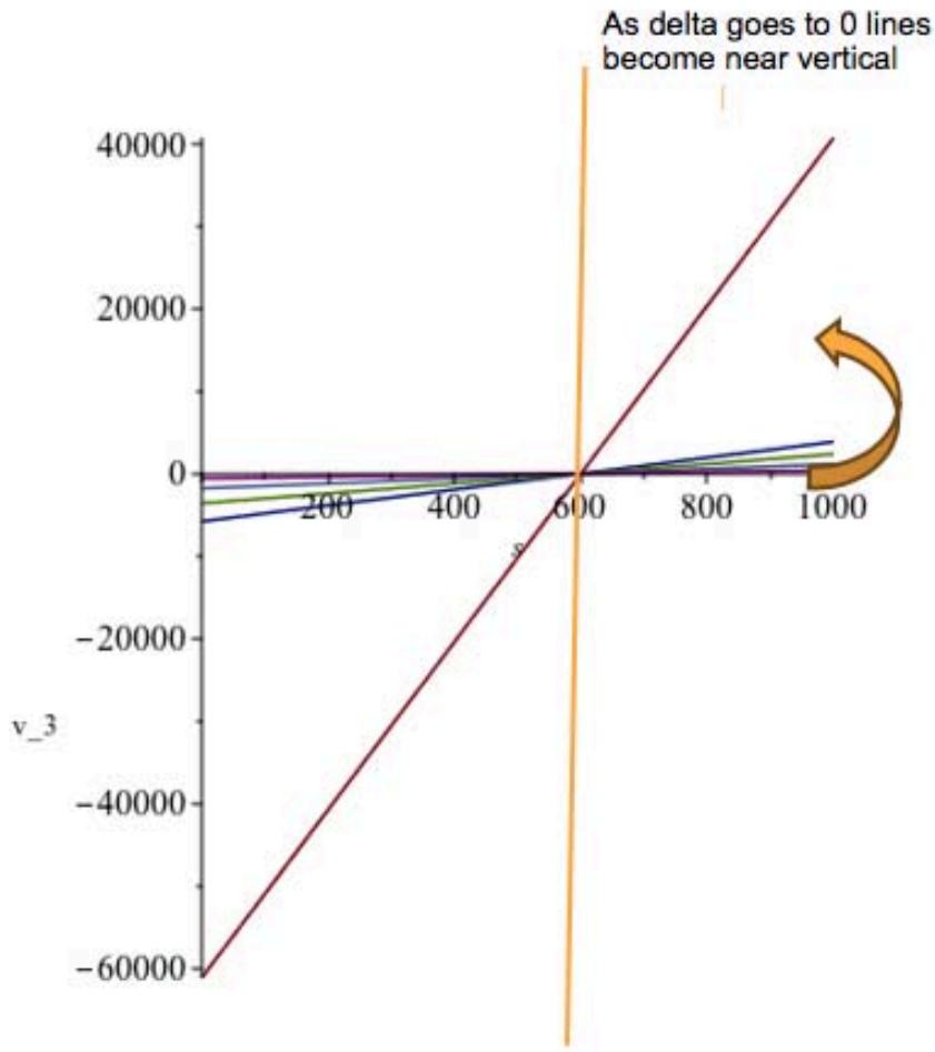 Figure 1c: Linear functions in the form $v_{3} = (-abs(b) + (m*s - 600), m > 0, b, \gamma$ -intercept. It is shown that the right side limit approaches infinity as $\delta \to 1$ Equation (l) is confirmed to provide the left hand limit at $s = s_0$. We have two problems here. One is the solution for the Euler equation when $\mu = 0$. The solution is obtained by solving for one of the constants $C_6$. There are six unknown constants in the solution of the above PDE when $\mu = 0$. ( $C_i, i = 1,2,\ldots,6$ ) We use the fact that in the space $\Im(y_3,s)$, the set $\{1,y_1,y_1^2\}$ is linearly independent, implying that all the constants are zero in the solution except $C_3$ and $C_4$ associated with variables $y_3, s$ respectively. The solution is expressed as linear sums of the spatial and time variables. Now $y_3$ is within an epsilon ball. The variable $\zeta$ appears in the initial condition when solving for the unknown constant $C_6$, and the initial condition for $v_3$ is given as the sum of arbitrarily large data $\zeta$ and sums of reciprocal degenerate Weierstrass P functions in the three directions for small $m$. We obtain the following solution, $$ \begin{array}{l} D _ {1} = \ln {\left(- 6 C _ {1} ^ {2} C _ {3} \zeta - 6 C _ {2} ^ {2} C _ {3} \zeta - 6 C _ {3} ^ {3} \zeta - 2 C _ {1} ^ {3} - 2 C _ {1} ^ {2} C _ {2} - 2 C _ {1} C _ {2} ^ {2} - 2 C _ {1} C _ {3} ^ {2} - 2 C _ {1} C _ {3} ^ {3}\right)} \\2 C _ {2} ^ {3} - 2 C _ {2} C _ {3} ^ {2} + \mathrm {e} ^ {C _ {3} ^ {2} C _ {4} C _ {5}}) C _ {3} \\D _ {2} = \left(1 2 (s + \zeta / 2) C _ {3} ^ {2} + 1 2 (C _ {1} / 6 + C _ {2} / 6) C _ {3} + 1 2 s \left(C _ {1} ^ {2} + C _ {2} ^ {2}\right)\right) \left(C _ {1} ^ {2} + C _ {2} ^ {2} + C _ {3} ^ {2}\right) \mathrm {e} ^ {- C _ {3} ^ {2} C _ {4} C _ {5}} \\\mathrm {C} _ {3} ^ {\quad 3} \mathrm {C} _ {4} \mathrm {C} _ {5} - \mathrm {C} _ {3} \\\end{array} $$ $$ v_{3}(\zeta,s) = \frac{1}{6 C_{3} (C_{1}^{2} + C_{2}^{2} + C_{3}^{2})} (- 2 C_{1}^{3} - 2 C_{1}^{2} C_{2} - 2 C_{1} C_{2}^{2} - 2 C_{1} C_{3}^{2} - 2 C_{2}^{3} - 2 C_{2} C_{3}^{2} + \mathrm{e}^{C_{3}^{2} C_{4} C_{5}} W \left(- \exp \left(\frac{D_{1} + D_{2}}{C_{3}}\right)\right) + \mathrm{e}^{C_{3}^{2} C_{4} C_{5}}) \end{array} $$ where $W$ is the Lambert $W$ function. We replaced $\zeta$ by $-\zeta +$ large shifts and found that the solution for $v_{3}$ for large $s$ (example $s = 600$ ), the solution is locally Hölder continuous with Hölder constant $1/3$ at arbitrary large values of $\zeta$. (specifically in plot shown, $\zeta = 10000$ ). In this analysis there is no restriction on the largeness of the data, thereby proving that the solution is admissible for arbitrary large data. The solution as seen in Figure 2 is not smooth from the first and higher derivatives in of $\zeta$. This is discussed further in the chapter as it pertains to the Onsager regularity problem particularly the endpoint regularity problem. See the following Figure 2, where the dashed line is the solution for $v_{3}$ and the non-dashed line is the Hölder solution, given for example as $$ (-0.52+(10000-\zeta)^{\frac{1}{3}}) $$ 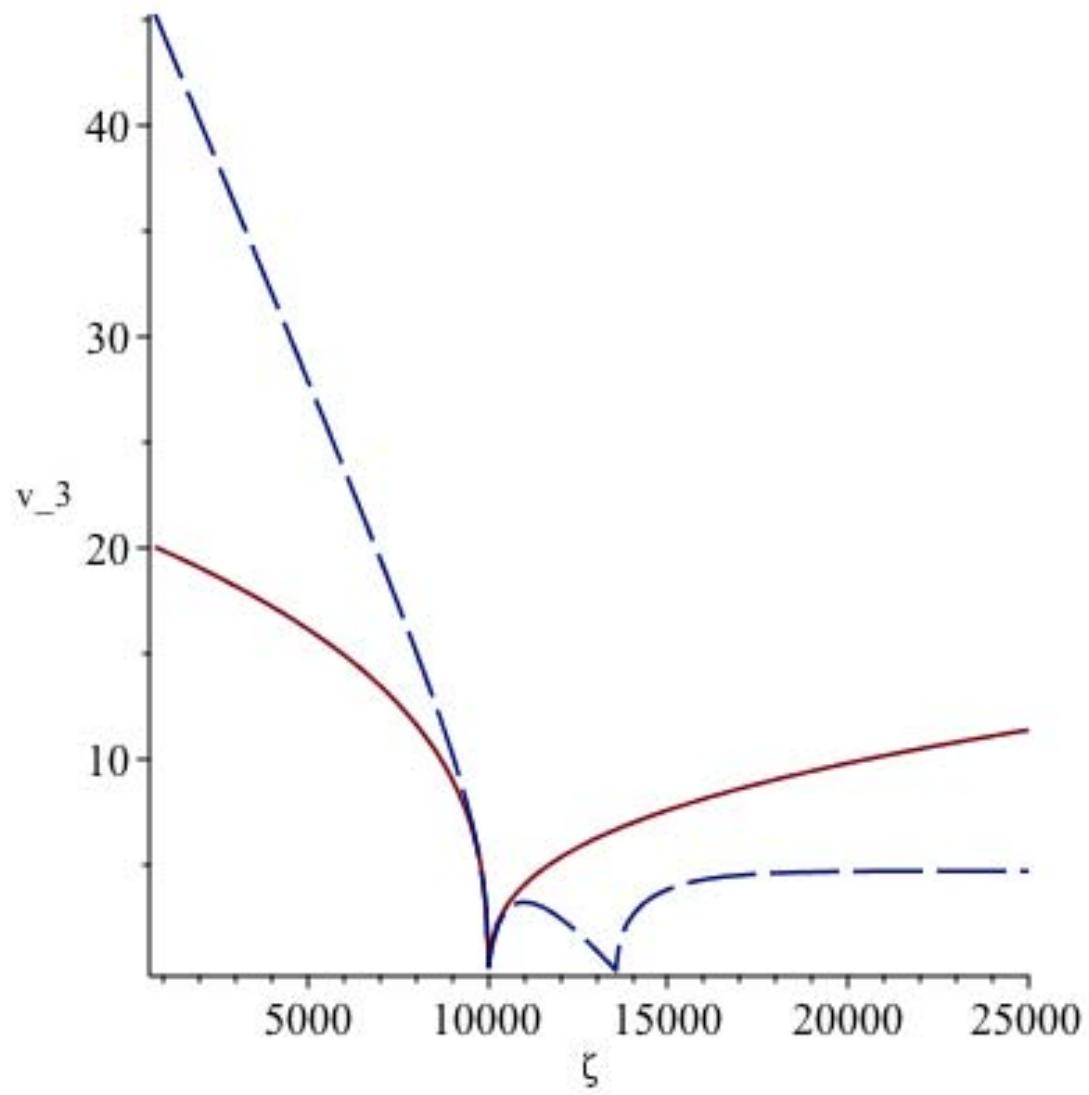 Figure 2: Locally Hölder continuous functions. $C_3 = -0.052C_4 = 0.05$ ## III. ON THE ENDPOINT REGULARITY IN ONSAGER'S CONJECTURE In order to obtain the solution previously shown as $v_{3}(\zeta, s)$ we let epsilon approach zero for solutions $v_{3}(\zeta, y_{3}, s)$ in the space $\Im(y_{3}, s)$. In this space a ball $B\left(y_{3c_{i}}; \varepsilon\right)$ exists with $\varepsilon > 0$. Here $\varepsilon$ is defined as a measure of how close one is to the center of a given cell in the lattice of the 3-Torus. Due to the definition of the space $\Im(y_{3}, s)$, the set $\{1, y_{1}, y_{1}^{2}\}$ is linearly independent, implying that all the constants are zero in the solution except $C_{3}$ and $C_{4}$ associated with variables $y_{3}, s$ respectively. The constants $C_{i}$ ranging from $i = 1..6$ in the solution of the Euler Equation (I) appear in the solution and in particular as an argument of the Lambert W function and is expressed as the following linear sum in spatial and time variables, $$ Y = C _ {1} y _ {1} + C _ {2} y _ {2} + C _ {3} y _ {3} + C _ {4} s + C _ {5} $$ Note that the solution can be obtained by solving Eq.(l) when $3\left(\frac{\partial v_3}{\partial y_3}\right)^2\rho - \left(\frac{\partial v_3}{\partial y_3}\right)^2 \approx 3\left(\frac{\partial v_3}{\partial y_3}\right)^2\rho$, that is for $\rho \gg 100\frac{kg}{m^3}$. It is found that an exact solution is given by Maple 2023 software when this approximation is made for large enough density. It is also worthy to note that for lower densities when we retain both terms in the previous approximation, that for the locally Hölder continuous functions in time $s$, with Hölder constant equal to exactly $1/3$, the product term $\left(\frac{\partial v_3}{\partial y_3}\right)^2\frac{\partial v_3}{\partial s}$ in Eq.(l) becomes independent of time $s$ and is only dependent on the spatial variables. The Onsager conjecture suggested the value $\alpha = 1/3$ for the case of the Euler equations but the conjecture was mainly considering only the Hölder regularity with respect to the space variables. Here we consider a combination of velocity-time conditions $(\zeta, s)$, which depend precisely on the Hölder exponent. As outlined in the introduction, P. Isett's proof shows that if $\alpha < 1/3$ (strictly less than) then conservation of energy fails. The works of Eyink[7,8] and Constantin, E, Titi [9] on the Onsager conjecture describe results in a Fourier setting and in a space called a Besov space (slightly larger than Hölder spaces), respectively. A well-known result is that if the velocity is a weak solution to the Euler equations such that, $$ u \in L ^ {3} (0, T; B _ {3} ^ {\alpha , \infty} (\mathbb {T} ^ {3})) \cap C (0, T; L ^ {2} (\mathbb {T} ^ {3})) $$ with $\alpha > 1/3$, (strictly greater than) then, $\|u(t)\| = \|u_0\|$, for all $t \in [0,T]$. This result is also true in Hölder spaces which was the setting that L. Onsager stated his conjecture rather than Besov spaces. Hölder continuous functions, as defined in Berselli [10] with a focus on space-time properties of functions with "homogeneous behavior", that is the one of the Hölder semi-norm $[. ]_{\alpha}$ (to be defined) and denote by $\dot{C}^{\alpha}$ the space of measurable functions such that this quantity is bounded. We say that, $$ u \in L ^ {\beta} (0, T; \dot {C} ^ {\alpha} (\mathbb {T} ^ {3})), $$ if there exists $f_{\alpha}\colon [0,T]\to \mathbb{R}^{+}$ such that 1) $|u(x,t) - u(y,t)|\leq f_{\alpha}(t)|x - y|^{\alpha},\forall x,y\in \mathbb{T}^{3}$, for a.e. $t\in [0,T]$ 2) $\int_0^T f_\alpha^\beta (t)dt < \infty$ and $f_{\alpha}(t) = [u(t)]_{\alpha}$ for almost all $t \in [0, T]$. The space is endowed with the semi-norm $$ \left\| u \right\| _ {L ^ {\beta} (0, T; \hat {C} ^ {\alpha} (\mathbb {T} ^ {3}))} := \left[ \int_ {0} ^ {T} f _ {\alpha} ^ {\beta} (t) d t \right] ^ {1 / \beta} $$ Finally $$ [ u ] _ {\alpha} := \sup _ {x \neq y} \frac {| u (x) - u (y) |}{| x - y | ^ {\alpha}} $$ In Berselli [10], (see Theorem 4.2 there) it is proven that if $u$ is a weak solution to the Euler equation (in usual form), such that $u \in L^{1 / \alpha}(0,T;\dot{C}_{\omega}^{\alpha}(\mathbb{T}^{3}))$ with $\alpha \in \left[\frac{1}{3},1\right]$ (where $\dot{C}_{\omega}^{\alpha}(\mathbb{T}^{3}) \subset C^{\alpha}(\mathbb{T}^{3})$ is the slightly smaller space defined through the norm $$ \| u \| _ {C _ {\omega} ^ {\alpha}} = \max _ {x \in \overline {{\mathbb {T}}} ^ {3}} | u (x) | + [ u ] _ {\omega , \alpha} $$ $$ [ u ] _ {\omega , \alpha} := \sup _ {x \neq y} \frac {| u (x) - u (y) |}{\omega (| x - y |) | x - y | ^ {\alpha}}, $$ with $\omega \colon \mathbb{R}^{+}\to \mathbb{R}^{+}$ a non-decreasing function such that $\lim_{s\to 0^{+}}\omega (s) = 0.$ ) then $u$ conserves the energy. In our proof of the endpoint regularity of Onsager's conjecture we are considering the Hölder continuous functions in the space $C^\alpha(\mathbb{T}^3)$. There are two steps here. First we set $v_{3}(y_{3}, s)$ equal to the variable $\zeta$ appearing in the initial condition when solving for the unknown constant $C_{6}$ where $\zeta > 0$, and recall that the initial condition for $v_{3}$ is given as the sum of arbitrarily large data $\zeta$ and sums of reciprocal degenerate Weierstrass P functions in the three directions for small $m$. (By reciprocal we mean that unity is divided by the Weierstrass P functions with a bounded periodic result.) In the second step we solve for $v_{3}(\zeta, y_{3}, s)$ for arbitrarily large negative data $\zeta < 0$. In both steps separately we keep $y_{3} \in B(y_{3c_{i}}; \varepsilon)$ and integrate the square associated with energy of solution $v_{3}(\zeta, y_{3}, s)$, that is we will show that our solution satisfies conservation of energy, (for all times $s \in [0, T)$ ). $$ \iint_ {C _ {2}} \int_ {y _ {3} = - \varepsilon} ^ {\varepsilon} v _ {3} ^ {2} (\zeta , y _ {3}, s) \mathrm {d} y _ {3} d y _ {1} d y _ {2} = \iiint_ {C (\vec {a}; \varepsilon)} v _ {3} ^ {2} (0) d y = \iiint_ {C (\vec {a}; \varepsilon)} (\zeta + (| y _ {1} | ^ {2} + | y _ {2} | ^ {2} + | y _ {3} | ^ {2})) ^ {2} d y $$ The integrals are carried out over a cube $C(\vec{a}; \varepsilon) = [-\varepsilon, \varepsilon]^3$, centered about $\vec{a}$. For $\varepsilon = 1/2$ the scaled solutions and hence graphs are shown in Figure 3 and 4. It is seen that in either step in both figures that energy is conserved thereby proving the endpoint regularity in Onsager's Conjecture. In Figure 3 and 4, the thicker part of curves hides the energy (E) at $s = 0$, behind the solution curve. For $\zeta > 0$ there are two curves coinciding and the same is true for $\zeta < 0$. The key empirical fact underlying the Onsager theory is the non-vanishing of turbulent energy dissipation in the zero-viscosity limit. The requirement for a non-vanishing limit of dissipation is that space-gradients of velocity must diverge. It is observed in experiment that when integrated over small balls or cubes in space the high-Reynolds limit of the kinetic energy dissipation rate defines a positive measure with multifractal scaling. The solution for Euler's equation given in this paper agrees with this fact that gradient of $v_{3}$ with respect to spatial position $y_{3}$ does in fact diverge. This is a short-distance/ultraviolet (UV) divergence in the language of quantum field-theory, or what Onsager himself termed a "violet catastrophe" [12]. Since the fluid equations of motion (I.1) contain diverging gradients, they become ill-defined in the limit. In order to develop a dynamical description which can be valid even as $\nu \rightarrow 0$, some regularization of this divergence must be introduced. 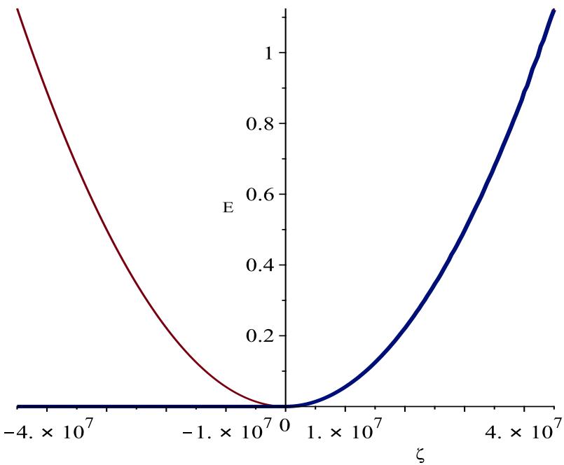 Figure 3: Energy of PNS system for arbitrarily large and positive data $\zeta$ 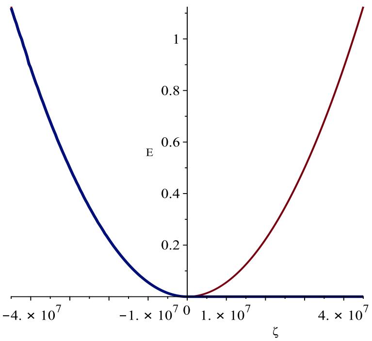 Figure 4: Energy of PNS system for arbitrarily large and negative data $\zeta$ In the book "Theory of unitary symmetry" by Rumer and Fet[12], the Laplacian is defined as an integration over a 3D-ball, in particular an epsilon ball. The viscous solution when $\mu$ is non-zero is subject to a rewriting of Eq (I) and to use this result first we integrate Eq.(I) over an $\varepsilon$ -ball, centered at each center of cells of the lattice of 3-Torus. Next using the divergence theorem for the term of Eq(I), that is specifically the expression $v_{3}\left(\frac{\partial^{2}v_{3}}{\partial y_{3}{}^{2}} +\frac{\partial^{2}v_{3}}{\partial y_{2}{}^{2}} +\frac{\partial^{2}v_{3}}{\partial y_{1}{}^{2}}\right)$, gives $\int_{y\in B_{\varepsilon}(y)}|\nabla v_3|^2 dy = 0$ where the surface integral is zero and since we are integrating a positive expression on an epsilon ball, at epsilon $= 0$ the integral is zero. Therefore Eq(I) becomes: $$ \left(\frac {\partial^ {3} v _ {3}}{\partial y _ {3}} ^ {3} + \frac {\partial^ {3} v _ {3}}{\partial y _ {3} \partial y _ {2}} ^ {2} + \frac {\partial^ {3} v _ {3}}{\partial y _ {3} \partial y _ {1}} ^ {2}\right) \mu (\delta - 1) + $$ $$ 1/6\left(3\rho v_{3}\frac{\partial^{2}v_{3}}{\partial y_{3}^{2}}+3\left(\frac{\partial v_{3}}{\partial y_{3}}\right)^{2}\rho-\left(\frac{\partial v_{3}}{\partial y_{ 3}}\right)^{2}+\frac{\partial^{2}v_{3}}{\partial y_{3}\partial y_{1}}+\frac{\partial^{2}v_{3}}{\partial y_{3}\partial y_{2}}\right)\frac{\partial v_{3}}{\partial s}=0 $$ Equation (II) is integrated over an epsilon ball so we solve Eq.(II) in a neighborhood of epsilon $= 0$ that is near the center of each cell of the lattice in the space $\Im(y_3, s)$. So we integrate Eq. (II) over an epsilon ball first and then take limit. We use the Fet theory on writing the Laplacian as an integral over an epsilon ball. Here we know that there is an operator $\Delta_{\varepsilon}v_{3} = \frac{3}{4\pi\varepsilon^{3}}\int v_{3}(y) - v_{3}(0)dy$ such that in the limit as epsilon approaches zero, $\frac{10}{\varepsilon^2}\Delta_{\varepsilon}v_{3} = \Delta v_{3}$. Integral is over epsilon ball centered at $\vec{a} = (a,b,c)$. We take the Taylor expansion around 0 (or center $\vec{a}$ to second order, which gives terms proportional to $y_{1}, y_{1}y_{2}$ and $y_{1}^{2}$, however due to the symmetry of the $y_{1}, y_{1}y_{2}$ related terms these integrate to zero over the ball and thus we have that, $$ \Delta_\varepsilon v_3 = \frac{3}{4\pi\varepsilon^3} \left[ \frac{1}{2} \frac{\partial^2 v_3}{\partial y_1^2} \int y_1^2 dy + \frac{1}{2} \frac{\partial^2 v_3}{\partial y_2^2} \int y_2^2 dy + \frac{1}{2} \frac{\partial^ 2 v_3}{\partial y_3^2} \int y_3^2 dy \right] + \mathcal{O}(\varepsilon^3) $$ where all derivatives are evaluated at the center $\vec{a}$. The integrals all give the same value, $$ \int y _ {1} ^ {2} d y = \frac {1}{3} \int y _ {1} ^ {2} + y _ {2} ^ {2} + y _ {3} ^ {2} d y = \frac {4 \pi}{3} \int_ {0} ^ {\varepsilon} r ^ {4} d r = \frac {4 \pi \varepsilon^ {5}}{1 5} $$ where the differential has been transformed to spherical coordinates in 3D. Substituting this into the main statement of the theorem, we obtain, $$ \Delta_{\varepsilon} v_{3} = \frac{3}{4\pi\varepsilon^{3}} \frac{4\pi\varepsilon^{5}}{15} \frac{1}{2} \left[ \frac{\partial^{2} v_{3}}{\partial y_{1}^{2}} + \frac{\partial^{2} v_{3}}{\partial y_{2}^{2}} + \frac{\partial^{2} v_{3}}{\partial y_{3}^{2}} \right] + \mathcal{O}(\varepsilon^{3}) = \frac{\varepsilon^{2}}{10} \Delta v_{3} + \mathcal{O}(\varepsilon^{3}) $$ Finally we take the limit, $$ \lim _ {\varepsilon \rightarrow 0} \frac {1 0}{\varepsilon^ {2}} \Delta_ {\varepsilon} v _ {3} = \lim _ {\varepsilon \rightarrow 0} [ \Delta v _ {3} + \mathcal {O} (\varepsilon) ] = \Delta v _ {3} $$ In Eq.(II) the Laplacian is differentiated wrt to $y_{3}$. Using Fet theory, where we integrate $\Delta_{\varepsilon} v_{3}$ on an epsilon ball centered at zero and generalized to the center of any cell center of the lattice of the 3-Torus, we obtain the following PDE for large density: $$ 1/6\left(3\rho v_{3}\frac{\partial^{2}v_{3}}{\partial y_{3}^{2}}+3\left(\frac{\partial v_{3}}{\partial y_{3}}\right)^{2}\rho+\frac{\partial^{2}v_{3}}{\partial y_{3}\partial y_{1}}+\frac{\partial^{2}v_{3}}{\partial y_{3}\partial y_{2}}\right)\frac{\partial v_{3}}{\partial s}+\mu(\delta-1)\frac{\partial v_{3}}{\partial y_{3}}=0 $$ with solution: $$ {v _ {3} =} {(1 / 3 - C _ {4} C _ {1} - C _ {4} C _ {2} + (- (6 C _ {1} y _ {1} + 6 C _ {2} y _ {2} + 6 C _ {3} y _ {3} + 6 C _ {4} s + 6 C _ {5}) C _ {3} C _ {4} ^ {2} C _ {5} \rho + 6 C _ {3} C _ {4} ^ {2} C _ {6} \rho -} $$ $$ 1 8 (C _ {1} y _ {1} + C _ {2} y + C _ {3} z + C _ {4} s + C _ {5}) ^ {2} C _ {3} C _ {4} \rho + C _ {1} ^ {2} C _ {4} ^ {2} + 2 C _ {1} C _ {2} C _ {4} ^ {2} + C _ {2} ^ {2} (C _ {4} ^ {2}) ^ {1 / 2}) / (C _ {3} C _ {4} \rho) $$ where $C_i$, $i = 1 \ldots 6$ are constants. Using the same initial condition in terms of $\zeta$ as in the first part in Eq(I), we can determine $C_6$ and on the space $\Im(y_3, s)$, all constants are zero and the only constants that survive are $C_3, C_4$ and arbitrarily large $\zeta$. When the two constants are as follows, $$ C _ {3} = 0. 0 5 2, C _ {4} = 0. 0 5 $$ for $\rho = 1000, \zeta = 10000$, the following result follows in Figure 5.  Figure 5: Locally Hölder continuous functions in $s$ Here it is clear that there exists a solution of PNS that is not smooth in time $s$ for the first and higher derivatives. Also if we specify the time, the solution is a Hölder continuous function in the data $\zeta$ with a Hölder constant equal to one half. The Full Equation Proof for the Periodic Navier Stokes Equations Integrating the Navier Stokes equations over an epsilon ball we obtain, $$ \int_{B_{y;\varepsilon}} \mathcal{G}_{\delta 1} + \mathcal{G}_{\delta 2} + \mathcal{G}_{\delta 4} \, dy = -\int_{B_{y;\varepsilon}} \mathcal{G}_{\delta 3} \, dy $$ The first part of $\mathcal{G}_3$ becomes, $$ \mathcal {G} _ {3} = \nabla \cdot \nabla (\Xi), $$ where $\nabla (\Xi) = \frac{1}{\rho}\Big(v_3^2\nabla_{y_1y_2}P + \vec{b} v_3\frac{\partial P}{\partial y_3}\Big)$ where $P$ is the pressure and $\rho$ is the density of the fluid. Dividing Eq.(IV) by the measure or volume of the ball of radius epsilon centered at point $a$. $$ B_{a;\varepsilon} $$ we know since $\Xi$ is continuous everywhere on the 3-Torus (since integrals are continuous in inverting gradient), and in particular at the center of the epsilon ball (note higher order derivatives of $v_{3}$ blowup, not $v_{3}$ and pressure), then, $$ \lim _ {\varepsilon \rightarrow 0} \frac{1}{| B _ {y ; \varepsilon} |} \int_ {B _ {a; \varepsilon}} \Xi (y) \, d y = \Xi (\mathrm{a}) \tag{V} $$ However using the Fet theory, we can see that the integral on the RHS of Eq.(IV) divided by the volume of the ball is related to the integral over the ball centered at $a$ of $\frac{1}{4\pi\varepsilon^2} (\Xi (y) - \Xi (a))$. Using Eq.(V), we obtain a difference of exactly zero so that we are left with, $$ \lim _ {\varepsilon \rightarrow 0} \frac {1}{| B _ {y ; \varepsilon} |} \int_ {B _ {a; \varepsilon}} \mathcal {G} _ {\delta 1} + \mathcal {G} _ {\delta 2} + \mathcal {G} _ {\delta 4} d y = 0 $$ $$ \int_{B_{a;\varepsilon}} \mathcal{G}_{\delta 1} + \mathcal{G}_{\delta 2} + \mathcal{G}_{\delta 4} \, dy = 0 $$ Eq.(VI) is the PDE we obtained previously and occurs at an arbitrarily small epsilon ball centered at each cell of the lattice of the 3-Torus. In reference [5], we showed that, $$ \mathcal {G} _ {\delta 1} + \mathcal {G} _ {\delta 2} + \mathcal {G} _ {\delta 4} = 3 \Phi (s) $$ Since the negative pressure gradients are greater than or equal to zero being reciprocal Weierstrass P functions and $v_{3}^{2} \geq 0$ and $v_{1}$ and $v_{2}$ cancel in the space $\Im (y_3,s)$ when integrating on the six faces of surface of a cell of $\mathbb{T}^3$, we have that, $$ \Phi (s) \geq 0 $$ and $$ \mathcal {G} _ {\delta 1} + \mathcal {G} _ {\delta 2} + \mathcal {G} _ {\delta 4} \geq 0 $$ Also $$ \Xi_ {2} = \frac {\| Q \|}{\| \vec {b} \|} = \frac {\left\| \frac {\partial v _ {3}}{\partial s} \vec {b} \cdot (\vec {b} \otimes \Delta v _ {3}) \right\|}{\| \vec {b} \|} $$ $$ \Xi_ {1} = \Xi + \Xi_ {2} $$ Recall that the three velocities are isotropic and they are continuous on $B_{a;\varepsilon}$ and $\Xi_2$ is continuous on the epsilon ball. Also $\Xi_2$ is independent of $s$ for Hölder continuous functions at $\alpha = 1/3$. Theorem $$ \mathcal {G} _ {\delta 1} + \mathcal {G} _ {\delta 2} + \mathcal {G} _ {\delta 4} = 0 \text {i f a n d o n l y i f} \Xi_ {1} \text {i s c o n t i n u o u s o n t h e e p s i l o n b a l l} $$ $$ B _ {a; \varepsilon}. $$ Proof: Apply (V) to $\Xi_1$ ## IV. CONCLUSION Satisfying a divergence free vector field and periodic boundary conditions respectively with a general spatiotemporal forcing term $f$ which is smooth and spatially periodic, the existence of solutions which blowup in finite time for PNS can occur starting with the first derivative and higher with respect to time. P. Isett (2016) (see [13]) has shown that the conservation of energy fails for the 3D incompressible Euler flows with Hölder regularity below 1/3. (Onsager's second conjecture) The endpoint regularity in Onsager's conjecture has been addressed, and it is found that conservation of energy occurs when the Hölder regularity is exactly 1/3. The solution for Euler's equation given in this paper agrees with this fact that gradient of $v_{3}$ with respect to spatial position $y_{3}$ does in fact diverge. This is a short-distance/ultraviolet (UV) divergence in the language of quantum field-theory as L. Onsager proposed. Finally very recent developed new governing equations of fluid mechanics are proposed to have no finite time singularities. This is the focus of the ongoing work of the author to be presented in the near future. Finally future work to conclude the nature of flows in a non-epsilon or arbitrary small ball for the 3-Torus will be carried out. ### ACKNOWLEDGEMENT I thank both reviewers for help with their insightful and valuable comments which were taken into consideration.

Generating HTML Viewer...

References

13 Cites in Article
Chaoqun Liu,Zhining Liu (2021). New governing equations for fluid dynamics.
Terry Moschandreou,Keith Afas (2021). Existence of Incompressible Vortex-Class Phenomena and Variational Formulation of Raleigh–Plesset Cavitation Dynamics.
T Moschandreou (2021). No Finite Time Blowup for 3D Incompressible Navier Stokes Equations via Scaling Invariance.
R Poisson Equation for Pressure.
Terry E. Moschandreou,Keith C. Afas (2023). Periodic Navier Stokes Equations for a 3D Incompressible Fluid with Liutex Vortex Identification Method.
Jean-Yves Chemin,Isabelle Gallagher,Ping Zhang (2019). Some remarks about the possible blow-up for the Navier-Stokes equations.
Gregory Eyink (1994). Energy dissipation without viscosity in ideal hydrodynamics I. Fourier analysis and local energy transfer.
Gregory Eyink (1995). Besov spaces and the multifractal hypothesis.
Peter Constantin,E Weinan,Edriss Titi (1994). Onsager's conjecture on the energy conservation for solutions of Euler's equation.
L Berselli (2023). Energy conservation for weak solutions of incompressible fluid equations: the H𝔬𝔬lder case and connections with Onsager's conjecture.
Lars Onsager (1945). The distribution of energy in turbulence.
B Yu,A I Rumer,Fet Theory of Unitary Symmetry.
Philip Isett (2018). A proof of Onsager's conjecture.
No ethics committee approval was required for this article type.
Data Availability
Not applicable for this article.
How to Cite This Article
T. E. Moschandreou. 2026. \u201cExploring Finite-Time Singularities and Onsager’s Conjecture with Endpoint Regularity in the Periodic Navier Stokes Equations\u201d. Global Journal of Research in Engineering - I: Numerical Methods GJRE-I Volume 23 (GJRE Volume 23 Issue I1).
Explore published articles in an immersive Augmented Reality environment. Our platform converts research papers into interactive 3D books, allowing readers to view and interact with content using AR and VR compatible devices.
Your published article is automatically converted into a realistic 3D book. Flip through pages and read research papers in a more engaging and interactive format.
Our website is actively being updated, and changes may occur frequently. Please clear your browser cache if needed. For feedback or error reporting, please email [email protected]
Thank you for connecting with us. We will respond to you shortly.