Loading menu…

Global Existence and Intrinsic Decay Rates for the Energy of a Kirchhoff Type in a Nonlinear Viscoelastic Equation

Send Message

To: Author

Global Existence and Intrinsic Decay Rates for the Energy of a Kirchhoff Type in a Nonlinear Viscoelastic Equation

Article Fingerprint

ReserarchID

6N1R3

Global Existence and Intrinsic Decay Rates for the Energy of a Kirchhoff Type in a Nonlinear Viscoelastic Equation Banner

Key Research Insights

Synthesized scholarly intelligence & interactive research assistant
  • English
  • Afrikaans
  • Albanian
  • Amharic
  • Arabic
  • Armenian
  • Azerbaijani
  • Basque
  • Belarusian
  • Bengali
  • Bosnian
  • Bulgarian
  • Catalan
  • Cebuano
  • Chichewa
  • Chinese (Simplified)
  • Chinese (Traditional)
  • Corsican
  • Croatian
  • Czech
  • Danish
  • Dutch
  • Esperanto
  • Estonian
  • Filipino
  • Finnish
  • French
  • Frisian
  • Galician
  • Georgian
  • German
  • Greek
  • Gujarati
  • Haitian Creole
  • Hausa
  • Hawaiian
  • Hebrew
  • Hindi
  • Hmong
  • Hungarian
  • Icelandic
  • Igbo
  • Indonesian
  • Irish
  • Italian
  • Japanese
  • Javanese
  • Kannada
  • Kazakh
  • Khmer
  • Korean
  • Kurdish (Kurmanji)
  • Kyrgyz
  • Lao
  • Latin
  • Latvian
  • Lithuanian
  • Luxembourgish
  • Macedonian
  • Malagasy
  • Malay
  • Malayalam
  • Maltese
  • Maori
  • Marathi
  • Mongolian
  • Myanmar (Burmese)
  • Nepali
  • Norwegian
  • Pashto
  • Persian
  • Polish
  • Portuguese
  • Punjabi
  • Romanian
  • Russian
  • Samoan
  • Scots Gaelic
  • Serbian
  • Sesotho
  • Shona
  • Sindhi
  • Sinhala
  • Slovak
  • Slovenian
  • Somali
  • Spanish
  • Sundanese
  • Swahili
  • Swedish
  • Tajik
  • Tamil
  • Telugu
  • Thai
  • Turkish
  • Ukrainian
  • Urdu
  • Uzbek
  • Vietnamese
  • Welsh
  • Xhosa
  • Yiddish
  • Yoruba
  • Zulu
Reading Preferences
Font Size
Line Spacing
Background
This converted HTML version may contain rendering inconsistencies. Please refer to the PDF for the authoritative version, or click here to provide feedback.

Abstract

In this work we consider a nonlinear hyperbolic equations of Kirch-hoff type in viscoelasticity. By using the potential well theory we obtain the existence of a global solution. Then, we prove the intrinsic decays for the energy of the nonlinear hyperbolic equations of Kirchhoff type in viscoelasticity of relaxation kernels described by the inequality for all with H convex.

I. INTRODUCTION

In this works, we study the global existence and intrinsic decay rates for the energy of a kirchhoff type in a nonlinear viscoelastic equation

(1.1){utt(x,t)−Φ(x)[μ(‖∇u(t)‖L2(Ω)2)Δu(x,t)−∫0th(t−s)Δu(x,s)ds]+but(x,t)=0,x∈Ω×R+∗

with initial data

(1.2)u(x,0)=u0(x),ut(x,0)=u1(x),x∈Ω,

and boundary conditions

(1.3)u(x,t)=0,(x,t)∈∂Ω×R+,

where Ω is a bounded domain in Rn, h(.):R+⟶R+ are given functions which will be spaced later and u0(x), u1(x) are given initial data belonging to appropriate space. All the parameter b are assumed to be positive constants. The function Φ(x) is the density, (ρ(x))−1=Φ(x), Φ(x)>0, for all x∈Ω, and

μ(s):=ξ0+ξ1sγ,

where s > 0, ξ0>0, ξ1>0 and γ≥1. For more information on using Kirchhoff type, see [4 - 6].

Also, a result of local existence for problem (1.1) - (1.3) for ξ1=0 has been proved in [1], for ξ1≠0, in the same way as [1], we get the same basic results for the local existence of problem (1.1) - (1.3) with a slight change in some calculations that do not affect the basic results.

The motivation of our work is due to some results regarding the following research papers: Boumaza, N and Boulaaras, S. [2] studied the general decay for Kirchhoff type in viscoelasticity with not necessarily decreasing kernel of (1.1)–(1.3). Marcelo M. Irena Lasiecka and Claudete M. Webler. [3] studied the intrinsic decay rates for the energy of a nonlinear viscoelastic equation modeling the vibrations of thin rods with variable density. M. M. Cavalcanti, V. N. Domingos Cavalcanti, I. Lasiecka and F. A. Falcao Nascimento. [7] studied the intrinsic decay rate estimates for the wave equation with competing viscoelastic and frictional dissipative effects.

I. Lasiecka, S. A. Messaoudi and M.

I. Mustafa. [8] studied the note on intrinsic decay rates for abstract wave equations with memory.

I. Lasiecka and X. Wang. [9] studied the intrinsic decay rate estimates for semilinear abstract second order equations with memory. Cavalcanti M. Filho VND. Cavalcanti JSP. Soriano JA. [10] studied the existence and uniform decay rates for viscoelastic problems with nonlinear boundary damping. For more results in this direction, see [11−15].

However, [1−3], [4−6] and [11−15] did not study the intrinsic decay rates for the energy of problem (1.1)–(1.3) of relaxation kernels described by the inequality h′(t)≤−H(h(t)) for all t≥0, with H convex. Motivated by the above research, we will consider the intrinsic decay rates for the energy of relaxation kernels described by the inequality h′(t)≤−H(h(t)) for all t≥0 of the model (1.1)–(1.3) in this paper.

The outline of the paper is as follows. In the second section we define the energy E(t) associated to (1.1) – (1.3) and show that it is a non-increasing function of t. In section 3, we prove global existence of solution of (1.1) – (1.3). Finally, in section 4, we prove the intrinsic decay rates for the energy of the posed problem.

II. ASSUMPTIONS AND MAIN RESULTS

In this section, we define the energy E(t) associated to (1.1)–(1.3) and show that it is a non-increasing function of t. We suppose that the kernel h(t) is a function satisfying

Assumptions 1

The relaxation function h:R+⟶R+ is a C1∩L1 decreasing function and satisfies

h(0)>0 and ∫0th(s)ds<ξ0.

Assumptions 2 (i) In addition to Assumption 1, we require

h′(t)≤−H(h(t)) for all t≥0,

where H∈C1(R+) which H(0)=0 is a given strictly increasing and convex function. Moreover,

H∈C2(0,∞) and limx→0+inf{x2H′′(x)−xH′(x)+H(x)}≥0.

(ii) With reference to the function H introduced above, let y(t) be the solution of the ODE

y′(t)+H(y(t))=0,y(0)=h(0)>0.

(iii) We assume that there exists α0∈[0,1) such that y1−α0∈L1(1,∞). In order to formulate the long-time behavior results, we recall the binary notation

(2.1){(h∗w)(t):=∫0th(t−s)w(s)ds,∫Ω(h∘w)(t)dx:=∫0th(t−s)‖w(x,s)−w(x,t)‖L2(Ω)2ds,(h⋄w)(t):=ρ(x)∫0th(t−s)(w(t)−w(s))ds.
E(t):=12‖ut(t)‖Lρ2(Ω)2+12(ξ0−∫0th(s)ds)‖∇u(t)‖L2(Ω)2
(2.2)+ξ12(γ+1)‖∇u(t)‖L2(Ω)2(γ+1)+12∫Ω(h∘∇u)(t)dx.

Note that, in view of (2.1), we have that

(2.3)0<l:=(ξ0−∫0∞h(s)ds)≤ξ0 for all (x,t)∈Ω×R+.

The energy satisfies the following identity

Lemma 1. We have the identity

(2.4)ddt{E(t)}=12∫Ω(h′∘∇u)(t)dx−12h(t)‖∇u(t)‖L2(Ω)2−b‖ut(t)‖Lρ2(Ω)2≤0.

Proof. Multiplying (1.1) by ρ(x)ut and integration over Ω, we have

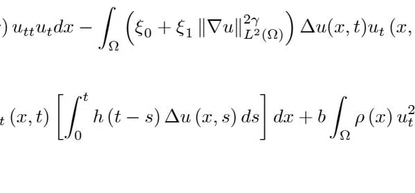
(2.5)∫Ωρ(x)uttutdx−∫Ω(ξ0+ξ1‖∇u‖L2(Ω)2γ)Δu(x,t)ut(x,t)dx+∫Ωut(x,t)[∫0th(t−s)Δu(x,s)ds]dx+b∫Ωρ(x)ut2(x,t)dx=0.

We have

∫Ωρ(x)uttutdx=12ddt{‖ut(t)‖Lρ2(Ω)2}.

And by using integration by parts, we have

−∫Ω(ξ0+ξ1‖∇u‖L2(Ω)2γ)Δu(x,t)ut(x,t)dx=−(ξ0+ξ1‖∇u‖L2(Ω)2γ)∫ΩΔu(x,t)ut(x,t)dx=(ξ0+ξ1‖∇u‖L2(Ω)2γ)∫Ω∇u(x,t).∇ut(x,t)dx=(ξ0+ξ1‖∇u‖L2(Ω)2γ)12ddt{∫Ω|∇u(x,t)|2dx}=ξ02ddt{‖∇u(t)‖L2(Ω)2}+ξ12‖∇u(t)‖L2(Ω)2γddt{‖∇u(t)‖L2(Ω)2}=ξ02ddt{‖∇u(t)‖L2(Ω)2}+ξ12(γ+1)ddt{‖∇u(t)‖L2(Ω)2(γ+1)}=ddt{12(ξ0+ξ1(γ+1)‖∇u(t)‖L2(Ω)2γ)‖∇u(t)‖L2(Ω)2}.

Notes

(2.7) And by using integration by parts, we have

∫Ωut(x,t)[∫0th(t−s)Δu(x,s)ds]dx=−∫0th(t−s)[∫Ω∇u(x,s).∇ut(x,t)dx]ds,

and using

−∇u(x,s).∇ut(x,t)=12ddt{|∇u(x,s)−∇u(x,t)|2}−12ddt{|∇u(x,t)|2},

then

∫Ωut(x,t)[∫0th(t−s)Δu(x,s)ds]dx=∫0th(t−s)∫Ω(12ddt{|∇u(x,s)−∇u(x,t)|2})dxds−∫0th(t−s)∫Ω(12ddt{|∇u(x,t)|2})dxds=12∫0th(t−s)(ddt{∫Ω|∇u(x,s)−∇u(x,t)|2dx})ds−12∫0th(t−s)(ddt{‖∇u(t)‖L2(Ω)2})ds,

by using (2.1), we get

Notes

(2.9)12∫0th(t−s)ddt{∫Ω|∇u(x,s)−∇u(x,t)|2dx}ds=12∫0tddt{h(t−s)(∫Ω|∇u(x,s)−∇u(x,t)|2dx)}ds−12∫0th′(t−s)(∫Ω|∇u(x,s)−∇u(x,t)|2dx)ds=12ddt{∫0th(t−s)∫Ω|∇u(x,s)−∇u(x,t)|2dxds}−12∫0th′(t−s)(∫Ω|∇u(x,s)−∇u(x,t)|2dx)ds=12ddt{∫Ω(h∘∇u)(t)dx}−12∫Ω(h′∘∇u)(t)dx,

and

−12∫0th(t−s)(ddt{‖∇u(t)‖L2(Ω)2})ds=−12(∫0th(t−s)ds)(ddt{‖∇u(t)‖L2(Ω)2})=−12(∫0th(s)ds)(ddt{‖∇u(t)‖L2(Ω)2})=−12ddt{(∫0th(s)ds)‖∇u(t)‖L2(Ω)2}+12h(t)‖∇u(t)‖L2(Ω)2.

By replacement (2.9) and (2.10) into (2.8), we get

∫Ωut(x,t)[∫0th(t−s)Δu(x,s)ds]dx=12ddt{∫Ω(h∘∇u)(t)dx}−12∫Ω(h′∘∇u)(t)dx−12ddt{(∫0th(s)ds)‖∇u(t)‖L2(Ω)2}+12h(t)‖∇u(t)‖L2(Ω)2=12ddt{∫Ω(h∘∇u)(t)dx−(∫0th(s)ds)‖∇u(t)‖L2(Ω)2}−12∫Ω(h′∘∇u)(t)dx+12h(t)‖∇u(t)‖L2(Ω)2.

By combining (2.6), (2.7) and (2.11) into (2.5), we get

12ddt{‖ut(t)‖Lρ2(Ω)2}+ddt{12(ξ0+ξ1(γ+1)‖∇u(t)‖L2(Ω)2γ)‖∇u(t)‖L2(Ω)2}+12ddt{∫Ω(h∘∇u)(t)dx−(∫0th(s)ds)‖∇u(t)‖L2(Ω)2}−12∫Ω(h′∘∇u)(t)dx+12h(t)‖∇u(t)‖L2(Ω)2+b‖ut(t)‖Lρ2(Ω)2=0,

Notes then

(2.12)ddt{12‖ut(t)‖Lρ2(Ω)2+12(ξ0−∫0th(s)ds)‖∇u(t)‖L2(Ω)2+ξ12(γ+1)‖∇u(t)‖L2(Ω)2(γ+1)+12∫Ω(h∘∇u)(t)dx}=12∫Ω(h′∘∇u)(t)dx−12h(t)‖∇u(t)‖L2(Ω)2−b‖ut(t)‖Lρ2(Ω)2,

by using (2.2) into (2.12), we get (2.4).

The proof of Lemma 1 is completes.

III. GLOBAL EXISTENCE

In this section we show that any solution of (1.1)−(1.3) is bounded and global, provided that E(0) is positive and small enough.

Theorem 1. Assume that (2.3) holds. Then the solution to problem (1.1) - (1.3) is bounded and global.

Proof. It suffices to show that ‖ut(t)‖Lρ2(Ω)2+‖∇u(t)‖L2(Ω)2 is bounded independently of t.

By using (2.3) and (A1) into (2.12), we get

ω1‖ut(t)‖Lρ2(Ω)2+ω2‖∇u(t)‖L2(Ω)2≤E(t)≤E(0),

where ω1>0 and ω2>0, then

‖ut(t)‖Lρ2(Ω)2+‖∇u(t)‖L2(Ω)2≤ω3E(0),

where ω3>0.

Then the solution to problem (1.1) - (1.3) is bounded and global.

The proof of Theorem 1 is completes.

 IV.  Decay of Solutions 

Now, we are in a position to state our main result.

Lemma 2. Let us assume that Assumption 1 and Assumption 2 are the place. Then, there exists a positive constant T0>0 such that

E((n+1)T)+H~(C9−1E((n+1)T))≤E(nT),n=1,2,3…,

for all T>T0 and all n∈N, where H~ is given in (4.49) and C9 is given in (4.52).

Proof. For this purpose, a by now standard procedure is to multiply (1.1) by the viscoelastic multiplier

(h⋄u)(t)=ρ(x)∫0th(t−s)(u(t)−u(s))ds,

and integrating over Ω×(nT,(n+1)T), we infer that

∫nT(n+1)T(utt(t),(h⋄u)(t))L2(Ω)dt−∫nT(n+1)T(Φ(x)(ξ0+ξ1‖∇u(t)‖L2(Ω)2γ)Δu(t),(h⋄u)(t))L2(Ω)dt+∫nT(n+1)T(Φ(x)(∫0th(t−s)Δu(s)ds),(h⋄u)(t))L2(Ω)dt+b∫nT(n+1)T(ut(t),(h⋄u)(t))L2(Ω)dt=0.

We shall analyze the above terms separately.

Direct calculation give

(utt(t),(h⋄u)(t))L2(Ω)=ddt{(ut(t),∫0th(t−s)(u(t)−u(s))ds)Lρ2(Ω)}−(ut(t),ddt(∫0th(t−s)(u(t)−u(s))ds))Lρ2(Ω)=ddt{(ut(t),∫0th(t−s)(u(t)−u(s))ds)Lρ2(Ω)}−(ut(t),(∫0th′(t−s)(u(t)−u(s))ds))Lρ2(Ω)−(ut(t),(∫0th(t−s)ut(t)ds))Lρ2(Ω),
∫nT(n+1)T(utt(t),(h⋄u)(t))L2(Ω)dt=(ut(t),∫0th(t−s)(u(t)−u(s))ds)Lρ2(Ω)|nT(n+1)T−∫nT(n+1)T(ut(t),∫0th′(t−s)(u(t)−u(s))ds)Lρ2(Ω)dt−∫nT(n+1)T(∫0th(s)ds)‖ut(x,t)‖Lρ2(Ω)2dt.

For the second term, by using integration by parts, we have

(4.3)−∫nT(n+1)T(Φ(x)(ξ0+ξ1‖∇u‖L2(Ω)2γ)Δu(t),(h⋄u)(t))L2(Ω)dt=−∫nT(n+1)T(ξ0+ξ1‖∇u‖L2(Ω)2γ)(Δu(t),∫0th(t−s)(u(t)−u(s))ds)L2(Ω)dt=∫nT(n+1)T(ξ0+ξ1‖∇u‖L2(Ω)2γ)(∇u(t),∫0th(t−s)(∇u(t)−∇u(s))ds)L2(Ω)dt.

Notes For the third term, by using integration by parts, we have

∫nT(n+1)T(Φ(x)∫0th(t−s)Δu(s)ds,(h⋄u)(t))L2(Ω)dt

Combining (4.2) - (4.4) into (4.1), we arrive at

\begin{array}{l} \left(u _ {t} (t), \int_ {0} ^ {t} h (t - s) (u (t) - u (s)) d s\right) _ {L _ {\rho} ^ {2} (\Omega)} \Bigg | _ {n T} ^ {(n + 1) T} \\- \int_ {n T} ^ {(n + 1) T} \left(u _ {t} (t), \int_ {0} ^ {t} h ^ {\prime} (t - s) (u (t) - u (s)) d s\right) _ {L _ {\rho} ^ {2} (\Omega)} d t \\- \int_ {n T} ^ {(n + 1) T} \left(\int_ {0} ^ {t} h (s) d s\right) \| u _ {t} (x, t) \| _ {L _ {\rho} ^ {2} (\Omega)} ^ {2} d t \\+ \int_ {n T} ^ {(n + 1) T} \left(\xi_ {0} + \xi_ {1} \| \nabla u \| _ {L ^ {2} (\Omega)} ^ {2 \gamma}\right) \left(\nabla u (t), \int_ {0} ^ {t} h (t - s) (\nabla u (t) - \nabla u (s)) d s\right) _ {L ^ {2} (\Omega)} d t \\+ \int_ {n T} ^ {(n + 1) T} \left\| \int_ {0} ^ {t} h (t - s) (\nabla u (t) - \nabla u (s)) d s \right\| _ {L ^ {2} (\Omega)} ^ {2} d t \\- \int_ {n T} ^ {(n + 1) T} \left(\int_ {0} ^ {t} h (t - s) \nabla u (t) d s, \int_ {0} ^ {t} h (t - s) (\nabla u (t) - \nabla u (s)) d s\right) _ {L ^ {2} (\Omega)} d t \\+ b \int_ {n T} ^ {(n + 1) T} \left(u _ {t} (t), (h \diamond u) (t)\right) _ {L ^ {2} (\Omega)} d t \\= 0, \end{array} \tag {4.}\tag{4.5}

then (4.5) is equivalent

Notes

(4.6)∫nT(n+1)T(∫0th(s)ds)‖ut(x,t)‖Lρ2(Ω)2dt=(ut(t),∫0th(t−s)(u(t)−u(s))ds)Lρ2(Ω)|nT(n+1)T−∫nT(n+1)T(ut(t),∫0th′(t−s)(u(t)−u(s))ds)Lρ2(Ω)dt+∫nT(n+1)T(ξ0+ξ1‖∇u‖L2(Ω)2γ)(∇u(t),∫0th(t−s)(∇u(t)−∇u(s))ds)L2(Ω)dt+∫nT(n+1)T‖∫0th(t−s)(∇u(t)−∇u(s))ds‖L2(Ω)2dt−∫nT(n+1)T(∫0th(t−s)∇u(t)ds,∫0th(t−s)(∇u(t)−∇u(s))ds)L2(Ω)dt+b∫nT(n+1)T(ut(t),(h⋄u)(t))L2(Ω)dt=J1+J2+J3+J4+J5+J6.

Estimate for|J1|, where

J1:=ut((n+1)T),∫0(n+1)Th((n+1)T−s)(u((n+1)T)−u(s))ds)Lρ2(Ω)−ut(nT),∫0nTh(nT−s)(u(nT)−u(s))ds)Lρ2(Ω).

Now, let m∈N be an arbitrary, natural number.

By using Young's inequality (for ε=1 ), we get

(4.7)ut(mT),∫0mTh(mT−s)(u(mT)−u(s))ds)Lρ2(Ω)=∫0mTh(mT−s)(ut(mT),(u(mT)−u(s)))Lρ2(Ω)ds≤∫0mTh(mT−s)[12‖ut(mT)‖Lρ2(Ω)2+12‖u(mT)−u(s)‖Lρ2(Ω)2]ds=12∫0mTh(mT−s)ds)‖ut(mT)‖Lρ2(Ω)2+12∫0mTh(mT−s)‖u(mT)−u(s)‖Lρ2(Ω)2ds,
(4.8)‖u(t)‖Lρ2(Ω)2≤‖ρ‖L2(Ω)2‖∇u(t)‖Lρ2(Ω)2,
(4.9)12∫0mTh(mT−s)‖u(mT)−u(s)‖Lρ2(Ω)2ds≤12‖ρ‖L2(Ω)2∫0mTh(mT−s)‖∇u(mT)−∇u(s)‖L2(Ω)2ds=12‖ρ‖L2(Ω)2∫Ω(h∘∇u)(mT)dx,

Notes by replacement (4.9) into (4.7) and using ∫0mTh(mT−s)ds=∫0mTh(s)ds, we get

ut(mT),∫0mTh(mT−s)(u(mT)−u(s))ds)Lρ2(Ω)
≤12∫0mTh(s)ds)‖ut(mT)‖Lρ2(Ω)2
+12‖ρ‖L2(Ω)2∫Ω(h∘∇u)(mT)dx,

by using (2.2), we get

(4.11){12‖ut(mT)‖Lρ2(Ω)2≤E(mT),and12∫Ω(h∘∇u)(mT)dx≤E(mT)

then, by combining (4.11) into (4.10), we get

ut(mT),∫0mTh(mT−s)(u(mT)−u(s))ds)Lρ2(Ω)≤∫0mTh(s)ds)E(mT)+‖ρ‖L2(Ω)2E(mT)≤{‖h‖L1(0,∞)+‖ρ‖L2(Ω)2}E(mT),
(4.12)|J1|≤C1[E((n+1)T)+E(nT)],
C1:=‖h‖L1(0,∞)+‖ρ‖L2(Ω)2.

Estimate for|J2|, where

J2:=−∫nT(n+1)T(ut(t),∫0th′(t−s)(u(t)−u(s))ds)Lρ2(Ω)dt.

By using Young's inequality (for ε=ε12 ), we get

(4.13)|J2|≤ε1∫nT(n+1)T‖ut(x,t)‖Lρ2(Ω)2dt+14ε1∫nT(n+1)T‖∫0th′(t−s)(u(t)−u(s))ds‖Lρ2(Ω)2dt.

Notes By using (4.8), Cauchy-Schwarz inequality and (2.1), we get

(4.14)∫nT(n+1)T‖∫0th′(t−s)(u(t)−u(s))ds‖Lρ2(Ω)2dt≤‖ρ‖L2(Ω)2∫nT(n+1)T‖∫0th′(t−s)(∇u(t)−∇u(s))ds‖L2(Ω)2dt≤−‖ρ‖L2(Ω)2h(0)∫nT(n+1)T∫0th′(t−s)‖∇u(t)−∇u(s)‖L2(Ω)2dsdt=−‖ρ‖L2(Ω)2h(0)∫nT(n+1)T∫Ω(h′∘∇u)(t)dxdt.

By replacement (4.14) into (4.13), we get

(4.15)|J2|≤ε1∫nT(n+1)T‖ut(x,t)‖Lρ2(Ω)2dt−14ε1‖ρ‖L2(Ω)2h(0)∫nT(n+1)T∫Ω(h′∘∇u)(t)dxdt.

Estimate|J3|, where

J3:=∫nT(n+1)T(ξ0+ξ1‖∇u‖L2(Ω)2γ)(∇u(t),∫0th(t−s)(∇u(t)−∇u(s))ds)L2(Ω)dt.

By using Young's inequality (for ε=ε22 ), we get

|J3|≤ε2∫nT(n+1)T(ξ0+ξ1‖∇u‖L2(Ω)2γ)2‖∇u(t)‖L2(Ω)2dt+14ε2∫nT(n+1)T‖∫0th(t−s)(∇u(t)−∇u(s))ds‖L2(Ω)2dt,

by using ‖∇u(t)‖L2(Ω)2γ≤(2(γ+1)ξ1E(0))2γ2(γ+1), we get

(4.17)ε2∫nT(n+1)T(ξ0+ξ1‖∇u‖L2(Ω)2γ)2‖∇u(t)‖L2(Ω)2dt≤ε2ξ0+ξ1(2(γ+1)ξ1E(0))2γ2(γ+1))2∫nT(n+1)T‖∇u(t)‖L2(Ω)2dt,

by using Cauchy-Schwarz inequality and (2.1), we get

‖∫0th(t−s)(∇u(t)−∇u(s))ds‖L2(Ω)2
≤(∫0th(t−s)ds)∫0th(t−s)‖∇u(t)−∇u(s)‖L2(Ω)2ds

Notes

(4.18)≤‖h‖L1(0,∞)∫Ω(h∘∇u)(t)dx,

by replacement (4.17) and (4.18) into (4.16), we get

|J3|≤ε2ξ0+ξ1(2(γ+1)ξ1E(0))2γ2(γ+1)∫nT(n+1)T‖∇u(t)‖L2(Ω)2dt
(4.19)+14ε2‖h‖L1(0,∞)∫nT(n+1)T∫Ω(h∘∇u)(t)dxdt.

Estimate|J4|, where

J4:=∫nT(n+1)T‖∫0th(t−s)(∇u(t)−∇u(s))ds‖L2(Ω)2dt.

By using (4.18), we get

(4.20)|J4|≤‖h‖L1(0,∞)∫nT(n+1)T∫Ω(h∘∇u)(t)dxdt.

Now, estimate|J5|, where

J5:=−∫nT(n+1)T(∫0th(t−s)∇u(t)ds,∫0th(t−s)(∇u(t)−∇u(s))ds)L2(Ω)dt.

By using Young's inequality (for ε=ε32 ), Cauchy-Schwarz inequality and (4.18), we get

|J5|≤ε3∫nT(n+1)T‖∫0th(t−s)∇u(t)ds‖L2(Ω)2dt
+14ε3∫nT(n+1)T‖∫0th(t−s)(∇u(t)−∇u(s))ds‖L2(Ω)2dt

Notes

(4.21)≤ε3‖h‖L1(0,∞)∫nT(n+1)T∫0th(t−s)‖∇u(t)‖L2(Ω)2dsdt+14ε3‖h‖L1(0,∞)∫nT(n+1)T∫Ω(h∘∇u)(t)dxdt=ε3‖h‖L1(0,∞)∫nT(n+1)T(∫0th(s)ds)‖∇u(t)‖L2(Ω)2dt+14ε3‖h‖L1(0,∞)∫nT(n+1)T∫Ω(h∘∇u)(t)dxdt.

Now, estimate|J6|, where

J6:=b∫nT(n+1)T(ut(t),(h⋄u)(t))L2(Ω)dt:=b∫nT(n+1)T(ut(t),∫0th(t−s)(u(t)−u(s))ds)Lρ2(Ω)dt.

By using Young's inequality (for ε=ε12 ), (4.8) and (4.18), we get

(4.22)|J6|≤b2ε1∫nT(n+1)T‖ut(t)‖Lρ2(Ω)2dt+14ε1∫nT(n+1)T‖∫0th(t−s)(u(t)−u(s))ds‖Lρ2(Ω)2dt≤b2ε1∫nT(n+1)T‖ut(t)‖Lρ2(Ω)2dt+14ε1‖ρ‖L2(Ω)2∫nT(n+1)T‖∫0th(t−s)(∇u(t)−∇u(s))ds‖L2(Ω)2dt≤b2ε1∫nT(n+1)T‖ut(t)‖Lρ2(Ω)2dt+14ε1‖ρ‖L2(Ω)2‖h‖L1(0,∞)∫nT(n+1)T∫Ω(h∘∇u)(t)dxdt.

Combining (4.12), (4.15) and (4.19)-(4.22) into (4.6), and recalling that ‖h‖L1(0,∞)<ξ0, we write

∫nT(n+1)T(∫0th(s)ds)‖ut(x,t)‖Lρ2(Ω)2dt
≤C1[E((n+1)T)+E(nT)]
+ε1∫nT(n+1)T‖ut(x,t)‖Lρ2(Ω)2dt−14ε1‖ρ‖L2(Ω)2h(0)∫nT(n+1)T∫Ω(h′∘∇u)(t)dxdt+ε2ξ0+ξ1(2(γ+1)ξ1E(0))2γ2(γ+1))2∫nT(n+1)T‖∇u(t)‖L2(Ω)2dt+14ε2ξ0∫nT(n+1)T∫Ω(h∘∇u)(t)dxdt+ξ0∫nT(n+1)T∫Ω(h∘∇u)(t)dxdt+ε3ξ0∫nT(n+1)T(∫0th(s)ds)‖∇u(t)‖L2(Ω)2dt+14ε3ξ0∫nT(n+1)T∫Ω(h∘∇u)(t)dxdt+b2ε1∫nT(n+1)T‖ut(t)‖Lρ2(Ω)2dt+14ε1ξ0‖ρ‖L2(Ω)2∫nT(n+1)T∫Ω(h∘∇u)(t)dxdt.

Notes

(4.23)

Since h(0)>0, we can select a points t1<T with t1 close to zero such that for all t≥t1

∫0th(s)ds≥t1h(t1):=c0.

Then (4.23) is equivalent

(4.24)∫nT(n+1)T{t1h(t1)−ε1(1+b2)}‖ut(x,t)‖Lρ2(Ω)2dt≤C1[E((n+1)T)+E(nT)]−14ε1‖ρ‖L2(Ω)2h(0)∫nT(n+1)T∫Ω(h′∘∇u)(t)dxdt+ε2ξ0+ξ1(2(γ+1)ξ1E(0))2γ2(γ+1))2∫nT(n+1)T‖∇u(t)‖L2(Ω)2dt+ξ0{14ε2+1+14ε3+14ε1‖ρ‖L2(Ω)2}∫nT(n+1)T∫Ω(h∘∇u)(t)dxdt+ε3ξ0∫nT(n+1)T(∫0th(s)ds)‖∇u(t)‖L2(Ω)2dt.

Now, multiplying (1.1) by ρ(x)u(x,t) and integrating over Ω×(nT,(n+1)T), we infer that

Notes

(4.25)∫nT(n+1)T(utt(t),u(t))Lρ2(Ω)dt−∫nT(n+1)T((ξ0+ξ1‖∇u‖L2(Ω)2γ)Δu(t),u(t))L2(Ω)dt+∫nT(n+1)T(∫0th(t−s)Δu(s)ds,u(t))L2(Ω)dt+b∫nT(n+1)T(ut(x,t),u(x,t))Lρ2(Ω)dt=0.

By using

utt(t)u(t)=ddt{ut(t)u(t)}−ut2(t),

we get

(4.26)∫nT(n+1)T(utt(x,t),u(x,t))Lρ2(Ω)dt(ut(t),u(t))Lρ2(Ω)|nT(n+1)T−∫nT(n+1)T‖ut(x,t)‖Lρ2(Ω)2dt.

By using integration by parts, we get

(4.27)−∫nT(n+1)T((ξ0+ξ1‖∇u‖L2(Ω)2γ)Δu(t),u(t))L2(Ω)dt=∫nT(n+1)T(ξ0+ξ1‖∇u‖L2(Ω)2γ)(∇u(t),∇u(t))L2(Ω)dt=∫nT(n+1)T(ξ0+ξ1‖∇u‖L2(Ω)2γ)‖∇u(t)‖L2(Ω)2dt.

By using integration by parts, we get

(4.28)∫nT(n+1)T(∫0th(t−s)Δu(s)ds,u(t))L2(Ω)dt=−∫nT(n+1)T∫0th(t−s)(∇u(s),∇u(t))L2(Ω)dsdt=∫nT(n+1)T∫0th(t−s)(∇u(t)−∇u(s),∇u(t))L2(Ω)dsdt−∫nT(n+1)T∫0th(t−s)(∇u(t),∇u(t))L2(Ω)dsdt=∫nT(n+1)T∫0th(t−s)(∇u(t)−∇u(s),∇u(t))L2(Ω)dsdt−∫nT(n+1)T(∫0th(s)ds)‖∇u(t)‖L2(Ω)2dt.
(4.29)b∫nT(n+1)T(ut(x,t),u(x,t))Lρ2(Ω)dt=b2∫nT(n+1)Tddt{‖u(x,t)‖Lρ2(Ω)2}dt=b2{‖u((n+1)T)‖Lρ2(Ω)2−‖u(nT)‖Lρ2(Ω)2}.

Notes By combining (4.26) - (4.29) into (4.25), we get

(4.30)(ut(t),u(t))Lρ2(Ω)|nT(n+1)T−∫nT(n+1)T‖ut(x,t)‖Lρ2(Ω)2dt+∫nT(n+1)T(ξ0+ξ1‖∇u‖L2(Ω)2γ)‖∇u(t)‖L2(Ω)2dt+∫nT(n+1)T∫0th(t−s)(∇u(t)−∇u(s),∇u(t))L2(Ω)dsdt−∫nT(n+1)T(∫0th(s)ds)‖∇u(t)‖L2(Ω)2dt+b2{‖u((n+1)T)‖Lρ2(Ω)2−‖u(nT)‖Lρ2(Ω)2}

Then (4.30) is equivalent

(4.31)−∫nT(n+1)T‖ut(x,t)‖Lρ2(Ω)2dt+∫nT(n+1)T(ξ0+ξ1‖∇u‖L2(Ω)2γ)‖∇u(t)‖L2(Ω)2dt=−(ut(t),u(t))Lρ2(Ω)|nT(n+1)T−∫nT(n+1)T∫0th(t−s)(∇u(t)−∇u(s),∇u(t))L2(Ω)dsdt+∫nT(n+1)T(∫0th(s)ds)‖∇u(t)‖L2(Ω)2dt−b2{‖u((n+1)T)‖Lρ2(Ω)2−‖u(nT)‖Lρ2(Ω)2}.
I1:=−(ut(t),u(t))Lρ2(Ω)|nT(n+1)T:=−(ut((n+1)T),u((n+1)T))Lρ2(Ω)+(ut(nT),u(nT))Lρ2(Ω).

By using Young's inequality (for ε=1 ), (4.8), 12‖ut(t)‖Lρ2(Ω)2≤E(t) and 12‖∇u(t)‖L2(Ω)2≤l−1E(t), we get

Notes

(ut(t),u(t))Lρ2(Ω)≤12‖ut(t)‖Lρ2(Ω)2+12‖u(t)‖Lρ2(Ω)2≤12‖ut(t)‖Lρ2(Ω)2+12‖ρ‖L2(Ω)2‖∇u(t)‖L2(Ω)2≤E(t)+‖ρ‖L2(Ω)2l−1E(t)={1+‖ρ‖L2(Ω)2l−1}E(t),

then

(4.32)|I1|≤C2{E((n+1)T)+E(nT)},

where

C2:=1+‖ρ‖L2(Ω)2l−1.

To estimate the term

I2:=−∫nT(n+1)T∫0th(t−s)(∇u(t)−∇u(s),∇u(t))L2(Ω)dsdt.

By using Young's inequality (for ε=ε42 ) and (2.1), we get

(4.33)|I2|≤14ε4∫nT(n+1)T∫0th(t−s)‖∇u(t)−∇u(s)‖L2(Ω)2dsdt+ε4∫nT(n+1)T∫0th(t−s)‖∇u(t)‖L2(Ω)2dsdt=14ε4∫nT(n+1)T∫Ω(h∘∇u)(t)dxdt+ε4∫nT(n+1)T(∫0th(s)ds)‖∇u(t)‖L2(Ω)2dt.
\begin{array}{r l} & {\mathrm{and} \frac {1}{2} \| \nabla u (t) \| _ {L ^ {2} (\Omega)} ^ {2} \leq l ^ {- 1} E (t), \mathrm{weget}} \\& {\qquad - \frac {b}{2} \left\{\| u ((n + 1) T) \| _ {L _ {\rho} ^ {2} (\Omega)} ^ {2} - \| u (n T) \| _ {L _ {\rho} ^ {2} (\Omega)} ^ {2} \right\}} \\& {\leq \frac {b}{2} \| \rho \| _ {L ^ {2} (\Omega)} ^ {2} \left\{\| \nabla u ((n + 1) T) \| _ {L ^ {2} (\Omega)} ^ {2} + \| \nabla u (n T) \| _ {L ^ {2} (\Omega)} ^ {2} \right\}} \\& {\leq b \| \rho \| _ {L ^ {2} (\Omega)} ^ {2} l ^ {- 1} \left\{E ((n + 1) T) + E (n T) \right\}} \\& {= C _ {2} ^ {\prime} \left\{E ((n + 1) T) + E (n T) \right\},} \end{array} \tag {4.8}\tag{4.34}
C2′:=b‖ρ‖L2(Ω)2l−1>0.

By combining (4.32) - (4.34) into (4.31), we can write

−∫nT(n+1)T‖ut(x,t)‖Lρ2(Ω)2dt+∫nT(n+1)T(ξ0+ξ1‖∇u‖L2(Ω)2γ)‖∇u(t)‖L2(Ω)2dt≤[C2+C2′]{E((n+1)T)+E(nT)}+14ε4∫nT(n+1)T∫Ω(h∘∇u)(t)dxdt+(ε4+1)∫nT(n+1)T(∫0th(s)ds)‖∇u(t)‖L2(Ω)2dt.

Notes

(4.35) On multiplied (4.24) by γ1 and multiplied (4.35) by γ2 and combining suitably, we get

(4.36)[γ1{t1h(t1)−ε1(1+b2)}−γ2]∫nT(n+1)T‖ut(x,t)‖Lρ2(Ω)2dt+γ2ξ0∫nT(n+1)T‖∇u(t)‖L2(Ω)2dt+γ2ξ1∫nT(n+1)T‖∇u‖L2(Ω)2(γ+1)dt≤{γ1C1+γ2[C2+C2′]}[E((n+1)T)+E(nT)]−γ114ε1‖ρ‖L2(Ω)2h(0)∫nT(n+1)T∫Ω(h′∘∇u)(t)dxdt+γ1ε2ξ0+ξ1(2(γ+1)ξ1E(0))2γ2(γ+1)∫nT(n+1)T‖∇u(t)‖L2(Ω)2dt+{γ1ξ0{14ε2+1+14ε3+14ε1‖ρ‖L2(Ω)2}+γ214ε4}∫nT(n+1)T∫Ω(h∘∇u)(t)dxdt+{γ1ε3ξ0+γ2(ε4+1)}∫nT(n+1)T(∫0th(s)ds)‖∇u(t)‖L2(Ω)2dt.

Let

(4.37){ε1:=t1h(t1)2(1+b2),ε2:=3εξ0γ1(ξ0+ξ1(2(γ+1)ξ1E(0))2γ2(γ+1))2,ε3:=εγ1ξ0,ε4:=2ε
(4.38){γ1:=4t1h(t1),γ2:=1

by using (4.37) and (4.38) into (4.36), we get

(4.39)∫nT(n+1)T‖ut(x,t)‖Lρ2(Ω)2dt+ξ0∫nT(n+1)T‖∇u(t)‖L2(Ω)2dt+ξ1∫nT(n+1)T‖∇u(t)‖L2(Ω)2(γ+1)dt≤C3[E((n+1)T)+E(nT)]−C4∫nT(n+1)T∫Ω(h′∘∇u)(t)dxdt+3εξ0∫nT(n+1)T‖∇u(t)‖L2(Ω)2dt+C5∫nT(n+1)T∫Ω(h∘∇u)(t)dxdt+(3ε+1)∫nT(n+1)T(∫0th(s)ds)‖∇u(t)‖L2(Ω)2dt,

where

C3:=γ1C1+C2+C2′,
{C4:=γ1(1+b2)2t1h(t1)‖ρ‖L2(Ω)2h(0),C5:=4ξ0t1h(t1){γ1ξ0+ξ1(2(γ+1)E(0)ξ1)2γ2(γ+1)12εξ0+1+γ1ξ04ε+(1+b2)2t1h(t1)‖ρ‖L2(Ω)2}+18ε

Adding and subtracting in (4.39) the term

−∫nT(n+1)T∫Ω(∫0th(s)ds)|∇u|2dxdtand∫nT(n+1)T∫Ωa(x)(h∘∇u)(t)dxdt,

in order to recover the energy E(t), we obtain

(1−3ε)∫nT(n+1)T∫Ω(ξ0−∫0th(s)ds)|∇u(t)|2dxdt
+∫nT(n+1)T‖ut(x,t)‖Lρ2(Ω)2dt+ξ1∫nT(n+1)T‖∇u(t)‖L2(Ω)2(γ+1)dt+∫nT(n+1)T∫Ω(h∘∇u)(t)dxdt≤C3[E((n+1)T)+E(nT)]+C5∫nT(n+1)T∫Ωk1(−h′∘∇u)(t)dxdt+C5∫nT(n+1)T∫Ω(h∘∇u)(t)dxdt,

(4.40) where

k1:=C4C5.

From (4·40), choosing ε sufficiently small, k1>0 and T large enough and using

α1{‖ut(t)‖Lρ2(Ω)2+‖∇u(t)‖L2(Ω)2+‖∇u(t)‖L2(Ω)2(γ+1)+∫Ω(h∘∇u)(t)dx}≤E(t)≤α2{‖ut(t)‖Lρ2(Ω)2+‖∇u(t)‖L2(Ω)2+‖∇u(t)‖L2(Ω)2(γ+1)+∫Ω(h∘∇u)(t)dx},

where

{α1:=12min{1,l,ξ1(γ+1)},andα2:=12max{1,ξ0,ξ1(γ+1)},

we get

(4.41)∫nT(n+1)TE(t)dt≤C6[E((n+1)T)+E(nT)]+C7∫nT(n+1)T∫Ω(h∘∇u)(t)dxdt+C7∫nT(n+1)T∫Ωk1(−h′∘∇u)(t)dxdt,
{C6:=α2C3min{(1−3ε)l,1,ξ1},andC7:=α2C5min{(1−3ε)l,1,ξ1}.

In the last step, we need to relate the viscoelastic energy to the viscoelastic damping. In the case when the relaxation function obeys a linear equation, this relation is straightforward and is expressed by a suitable multiplication. However, in the case of general decays, additional arguments are used. Here, we follow [17]. From the assumption 2 made on the viscoelastic kernel h and from [17,Lemma4] we obtain

(4.42)(h∘∇u)(t)≤H^α−1(−h′∘∇u)(t),t∈[nT,(n+1)T],
Hα(s)=αs1−1αH(1sα),
supt>0∫0th1−α(t−s)‖∇u(t)−∇u(s)‖2ds<∞.
∫nT(n+1)TE(t)dt≤C6[E((n+1)T)+E(nT)]
(4.43)+C7∫nT(n+1)T∫Ω[H^−1+k1](−h′∘∇u)(t)dxdt.

Next, we shall employ the following version of Jensen's inequality applied to measures and convex functions F. Let F be a convex increasing function on [α,b], let f:Ω⟼[α,b], and let h be an integrable function such that h(x)≥0 and

∫Ωh(x)dx=h0>0.

Then, we have

(4.44)∫ΩF−1(f(x))h(x)dx≤h0F−1[h0−1∫Ωf(x)h(x)dx].

We shall use (4.44) in order to bring the functions H in front of the integrals. Let us denote

α0:= meas (Ω).

We note that the function H^−1+k1 is concave. Let

{F−1=H^−1+k1,f(x)=(−h′∘∇u)(t),h(x)=T,h0=Tα0,h0−1=α0−1T−1

thus, we have

(4.45)∫nT(n+1)T∫Ω[H^−1+k1](−h′∘∇u)(t)dxdt≤α0T[H^−1+k1][α0−1T−1∫nT(n+1)T∫Ω(−h′∘∇u)(t)dxdt].

On the other hand, from the identity (2.4) for the energy, we can write

E((n+1)T)−E(nT)=12∫nT(n+1)T{∫Ω(h′∘∇u)(t)dx−h(t)‖∇u(t)‖L2(Ω)2−2b‖ut(t)‖Lρ2(Ω)2}dt=−∫nT(n+1)TD(t)dt,

where

(4.46)D(t):=12{∫Ω(−h′∘∇u)(t)dx+h(t)‖∇u(t)‖L2(Ω)2+2b‖ut(t)‖Lρ2(Ω)2}.

En replacement (4.45) into (4.43) and using

(4.47)E(nT)=E((n+1)T)+∫nT(n+1)TD(t)dt,

we get

∫nT(n+1)TE(t)dt≤C6{2E((n+1)T)+∫nT(n+1)TD(t)dt}+C7α0T[H^−1+k1][α0−1T−1∫nT(n+1)T∫Ω(−h′∘∇u)(t)dxdt],

and using (4.46) we get

∫nT(n+1)T∫Ω(−h′∘∇u)(t)dxdt≤2∫nT(n+1)TD(t)dt,

thus, we get

Notes

(4.48)∫nT(n+1)TE(t)dt≤C6{2E((n+1)T)+∫nT(n+1)TD(t)dt}+2C7α0T[H^−1+k1][α0−1T−1∫nT(n+1)TD(t)dt]=2C6E((n+1)T)+C6∫nT(n+1)TD(t)dt+2C7α0T[H^−1+k1][α0−1T−1∫nT(n+1)TD(t)dt]≤2C6E((n+1)T)+C8[H^−1+k2][∫nT(n+1)TD(t)dt]=2C6E((n+1)T)+C8H~−1[∫nT(n+1)TD(t)dt],

where

(4.49){C8:=max{2C7,1},H~:=[H^−1+k2]−1,k2:=(C6+2C7k1).

By integrating t to (n+1)T on both sides of the inequality ddt{E(t)}≤0 yields

(4.50)E((n+1)T)≤E(t) for all (n+1)T≥t,

integrating (4.50) from nT to (n+1)T yields

(4.51)∫nT(n+1)TE(t)dt≥∫nT(n+1)TE((n+1)T)dt=∫nT(n+1)TdtE((n+1)T)=TE((n+1)T),

by replacement (4.51) into (4.48), we get

TE((n+1)T)≤2C6E((n+1)T)+C8H~−1[∫nT(n+1)TD(t)dt],
(T−2C6)E((n+1)T)≤C8H~−1[∫nT(n+1)TD(t)dt].

For T large enough, where C6 is a positive constant, which implies that

E((n+1)T)≤C9H~−1[∫nT(n+1)TD(t)dt],

where

(4.52)C9:=C8(T−2C6),

which gives that

Notes

(4.53)H~(C9−1E((n+1)T))≤∫nT(n+1)TD(t)dt,

by using (4.47) into (4.53), we get

H~(C9−1E((n+1)T))≤E(nT)−E((n+1)T),

from the above we have

E((n+1)T)+H~(C9−1E((n+1)T))≤E(nT),n=1,2,3....

Then the Proof of Lemma 2 is complete.

Lemma 3. Let p be a positive, increasing function such that p(0)=0. Since p is increasing, we can define an increasing function q, q(x)≡x−(I+p)−1(x). Consider a sequence Fn of positive numbers which satisfies

(4.54)Fm+1+p(Fm+1)≤Fm.

Then Fm≤S(m) where S(t) is a solution of the differential equation

(4.55)ddt{S(t)}+q(S(t))=0,S(0)=F0.

Moreover, if p(x)>0 for x>0 then limt→∞S(t)=0.

Proof. Proof of the Lemma use the proof retraction. Assume Fm≤S(m) and prove that Fm+1≤S(m+1).

Inequality (4.54) is equivalent to

(I+p)Fm+1≤Fm,

and since (I+p)−1 is monotone increasing, Fm+1≤(I+p)−1Fm, and using

(I+p)−1Fm=(I−q)Fm,
(4.56)Fm+1≤(I−q)Fm=Fm−q(Fm).

On the other hand, since q is an increasing function, the solution S(t) of equation (4.55) is described by a nonlinear contraction.

In particular integrating ddt{S(t)}≤0 from m to τ yields

(4.57)S(τ)≤S(m) for all t≥τ.

Integrating equation (4.55) from m to (m+1) yields

(4.58)S(m+1)−S(m)+∫mm+1q(S(τ))dτ=0.

Since q is increasing, by using (4.57) we obtain for all m≤τ≤m+1

Notes

∫mm+1q(S(τ))dτ≤∫mm+1q(S(m))dτ=q(S(m))∫mm+1dτ=q(S(m)),

then

(4.59)−∫mm+1q(S(τ))dτ≥−q(S(m)), for all m≤τ≤m+1,

by replacement (4.59) into (4.58) and using the inductive assumption Fm≤S(m), we get

(4.60)S(m+1)≥S(m)−q(S(m))=(I−q)S(m)≥(I−q)Fm=Fm−q(F(m)),

comparing (4.60) with (4.56) yields

S(m+1)≥Fm+1.

Then the Proof of Lemma 3 is complete.

Theorem 2. Let us assume that Assumption 1 and Assumption 2 are the place. Then there exist positive constants c1,c2 and T0 such that the solution of problem (1.1) - (1.3) satisfies E(t)≤s(t), where s(t) verifies the ODE

st+H^(s)=0,s(0)=E(0),t≥T0>0,

with H^(s)=c1H(c2s).

Proof. Thus, we are in a position to apply the result of Lemma 2 with

Fm≡E(mt),F0≡E(0).

This yields

E(mT)≤S(m),m=0,1,2,3....

Setting t=mT+τ and recalling the evolution property gives

E(t)≤E(mT)≤S(m)≤S(t−τT)≤S(tT−1),

which completes the proof of Theorem 2.

References

27 Cites in Article
  1. 1. Mohamed Medjden,Nasser-Eddine Tatar (2005). Asymptotic behavior for a viscoelastic problem with not necessarily decreasing kernel. Applied Mathematics and Computation, 167(2), 1221-1235.
  2. 2. Nouri Boumaza,Salah Boulaaras (2018). General decay for Kirchhoff type in viscoelasticity with not necessarily decreasing kernel. Mathematical Methods in the Applied Sciences, 41(16), 6050-6069.
  3. 3. M Marcelo,Cavalcanti,N Valéria,Irena Cavalcanti,Lasiecka,M Claudete,Webler (2016). Intrinsic decay rates for the energy of a nonlinear viscoelastic equation modeling the vibrations of thin rods with variable density. Adv. Nonlinear Anal, aop.
  4. 4. Chunlai Mu,Jie Ma (2013). On a system of nonlinear wave equations with Balakrishnan–Taylor damping. Zeitschrift für angewandte Mathematik und Physik, 65(1), 91-113.
  5. 5. Nasser-Eddine Tatar,Abderrahmane Zaraï (2011). Exponential stability and blow up for a problem with Balakrishnan–Taylor damping. Demonstratio Mathematica, 44(1), 67-90.
  6. 6. N Tatar,A -E.; Zara,S Abdelmalek (2013). Elastic membrane equation with memory term and nonlinear boundary damping: global existence decay and blow-up of the solution. Acta Mathematica Scientia, 33(1), 84-106.
  7. 7. M Cavalcanti,V Domingos Cavalcanti,I Lasiecka,F Falcoo Nascimento (2014). Intrinsic decay rate estimates for the wave equation with competing viscoelastic and frictional dissipative effects. Discrete Contin. Dyn. Syst. Ser. B, 19(7), 1987-2012.
  8. 8. Irena Lasiecka,Salim Messaoudi,Muhammad Mustafa (2013). Note on intrinsic decay rates for abstract wave equations with memory. Journal of Mathematical Physics, 54(3), 31504.
  9. 9. Irena Lasiecka,Xiaojun Wang (2014). Intrinsic Decay Rate Estimates for Semilinear Abstract Second Order Equations with Memory. Springer INdAM Series, 10, 271-303.
  10. 10. M Cavalcanti,Vnd Filho,Jsp Cavalcanti,J Soriano (2001). Existence and uniform decay rates for viscoelastic problems with nonlinear boundary damping. Differential Integral Equ, 14, 85-116.
  11. 11. M Cavalcanti,M Aassila,J Soriano (2000). Asymptotic stability and energy decay rates for solutions of the wave equation with memory in a star-shaped domain. SIAM J. Control Opt, 38(5), 1581-1602.
  12. 12. W Hrusa (1985). Global existence and asymptotic stability for a nonlinear hyperbolic Volterra equation with large initial data. SIAM J. Math. Anal, 16, 110-134.
  13. 13. M Medjden,N.-E Tatar On the wave equation with a temporal non-local term and a weak dissipation. On the wave equation with a temporal non-local term and a weak dissipation
  14. 14. Michael Renardy (1988). Coercive estimates and existence of solutions for a model of one- dimensional viscoelasticity with a non-integrable memory function. Journal of Integral Equations and Applications, 1(1), 7-16.
  15. 15. Qin Tiehu (1999). Asymptotic Behavior of a Class of Abstract Semilinear Integrodifferential Equations and Applications. Journal of Mathematical Analysis and Applications, 233(1), 130-147.
  16. 16. Constantine Dafermos (1970). Asymptotic stability in viscoelasticity. Archive for Rational Mechanics and Analysis, 37(4), 297-308.
  17. 17. Irena Lasiecka,Xiaojun Wang (2014). Intrinsic Decay Rate Estimates for Semilinear Abstract Second Order Equations with Memory. Springer INdAM Series, 10, 271-303.
  18. 18. Irena Lasiecka,Xiaojun Wang (2015). Moore–Gibson–Thompson equation with memory, part II: General decay of energy. Journal of Differential Equations, 259(12), 7610-7635.
  19. 19. A Love (1944). A Treatise on the Mathematical Theory of Elasticity. A Treatise on the Mathematical Theory of Elasticity
  20. 20. Salim Messaoudi,Nasser‐eddine Tatar (2007). Global existence and uniform stability of solutions for a quasilinear viscoelastic problem. Mathematical Methods in the Applied Sciences, 30(6), 665-680.
  21. 21. S Messaoudi,N.-E Tatar (2008). Exponential and polynomial decay for a quasilinear viscoelastic equation. Nonlinear Anal, 68(4), 785-793.
  22. 22. Salim Messaoudi,Nasser‐eddine Tatar (2009). Exponential decay for a quasilinear viscoelastic equation. Mathematische Nachrichten, 282(10), 1443-1450.
  23. 23. Jaime Muñoz Rivera,Alfonso Peres Salvatierra (2001). Asymptotic behaviour of the energy in partially viscoelastic materials. Quarterly of Applied Mathematics, 59(3), 557-578.
  24. 24. Muhammad Mustafa,Salim Messaoudi (2012). General stability result for viscoelastic wave equations. Journal of Mathematical Physics, 53(5), 53702.
  25. 25. Jan Prüss (2009). Decay properties for the solutions of a partial differential equation with memory. Archiv der Mathematik, 92(2), 158-173.
  26. 26. D Russell (1978). Controllability and stabilizability theory for linear partial differential equations: Recent progress and open questions. SIAM Rev, 20(4), 639-739.
  27. 27. T Qin (1999). Asymptotic behavior of a class of abstract semilinear integrodi¤erential equations and applications. J. Math. Anal. Appl, 233(1), 130-147.

Funding

No external funding was declared for this work.

Conflict of Interest

The authors declare no conflict of interest.

Ethical Approval

No ethics committee approval was required for this article type.

Data Availability

Not applicable for this article.

How to Cite This Article

Draifia Alaeddine. 2021. "Global Existence and Intrinsic Decay Rates for the Energy of a Kirchhoff Type in a Nonlinear Viscoelastic Equation". Global Journal of Science Frontier Research - F: Mathematics & Decision GJSFR-F Volume 21 (GJSFR Volume 21 Issue F1).

More Citation Formats

Download Citation

Journal Specifications

Crossref Journal DOI 10.17406/GJSFR

Print ISSN 0975-5896

e-ISSN 2249-4626

Keywords
Classification
GJSFR-F Classification MSC 2010: 47N70
Version of record
v1.2

Issue date
February 12, 2021

Language
English
Order Article Reprint
Experience in AR

Explore published articles in an immersive Augmented Reality environment. Our platform converts research papers into interactive 3D books, allowing readers to view and interact with content using AR and VR compatible devices.

Read in 3D

Your published article is automatically converted into a realistic 3D book. Flip through pages and read research papers in a more engaging and interactive format.

Article Matrices
Total Views: 697
Total Downloads: 53
All Trends

Request Access

Please fill out the form below to request access to this research paper. Your request will be reviewed by the editorial or author team.
X

This is the heading

Lorem ipsum dolor sit amet, consectetur adipiscing elit. Ut elit tellus, luctus nec ullamcorper mattis, pulvinar dapibus leo.

High-quality academic research articles on global topics and journals.

Global Existence and Intrinsic Decay Rates for the Energy of a Kirchhoff Type in a Nonlinear Viscoelastic Equation

Draifia Alaeddine
Draifia Alaeddine