Half - Step Implicit Linear Multistep Hybrid Block Third Derivative Methods of Order Four for the Solution of Third order Ordinary Differential Equations

Skwame, Yusuf; Raymond, Dominic; Tumba, Pius; Adiku, Lydia

I. INTRODUCTION

This paper considers third order initial value problems of the form

Where f is continuous within the interval of integration, solving higher order derivatives method by reducing them to a system of first-order approach involves more functions to evaluate which then leads to a computational burden as in Kayode and Obuarhua (2013) and James et al. (2013). Various approaches have been proposed to find the analytic solution of (1) ranging from predictor-corrector method to hybrid methods. Despite the success recorded by the predictor-corrector methods, its major setback is that the predictor are in reducing order of accuracy especially when the value of the step-length is high and moreover the result are at overlapping interval. The hybrid method was established to circumvent the Dahlquist barrier theorem which gives a better approximation to solutions of initial value problems of stiff ordinary differential equations than the k-step method.

Scholars who recently adopted the hybrid method other than the direct method in approximating (1) include among others Adesanya et al. (2013), Adebayo and

Adebola (2016), Adoghe and Omole (2019), Kuboye and Omar (2015), Olabode and Momoh (2016), Kayode and Adeyeye (2011) and Mohammed and Adeniyi (2014). We adopted the method of collocation and interpolation of the power series approximation as the basis function to generate continuous linear multistep method as other scholars in solving (1). The derivation of continuous linear multistep methods for direct solution of ordinary differential equations have been discussed over the years in literature and these include, among others collocation, interpolation, integration, interpolating polynomials and basis functions such as, Chebyshev polynomials, trigonometric functions, exponential functions.

In this paper, we developed half-step third derivative hybrid block method of order four with two cases for direct solution of third order ordinary differential equation which is implemented in block. The method developed evaluates less function per step and circumventing the Dahlquist barrier's by introducing a hybrid points.

The paper is organized as follows: First is a discussion of the new half-step third derivative hybrid block method and the materials for the development of the method. This is followed by a consideration of analysis of the basic properties of the new half-step third derivative hybrid block method, which include convergence, stability region, numerical experiments where the efficiency of the derived method is tested on some stiff numerical examples and discussion of results. Lastly, the study concludes by comparing the results obtained with an existing work of Adeyeye and Omar (2018), Adebayo and Adebola (2016), Adoghe and Omole (2019) and Mohammed and Adeniyi (2014).

II. DERIVATION OF THE NEW HALF-STEP HYBRID BLOCK METHOD

In this section we intend to develop a family of half-step third derivative hybrid method with three hybrid points $u, v$ and $w$ , which are all rational numbers $u, v, w \in \left[0, \frac{1}{2}\right]$ of the form

$\alpha_{0}(t), \alpha_{u}(t), \alpha_{v}(t), \beta_{j}(t), \beta_{u}(t), \beta_{v}(t), \beta_{w}(t)$ are polynomials, $y_{n+j} = y\left(x_{n+j}\right)$ , $f_{n+j} = f\left(x_{n+j}, y_{n+j}\right)$ $t = \frac{x - x}{h}$ . Consider the power series approximate solution of the form

where r=3 and s=5 are the numbers of interpolation and collocation points respectively, is considered to be a solution to (1).

The third derivative of (3) gives

Substituting (4) into (1) gives

Collocating (5) at all points $x_{n+s,s}=0,u,v,w,\frac{1}{2}$ and Interpolating Equation (3) at $x_{n+r},r=0,u,v$ , gives a system of non linear equation of the form

Notes

Where

Solving (6) for $a_i$ 's using Gaussian elimination method, gives a continuous hybrid linear multistep method of the form

Differentiating (7) twice yields

We then impose the following conditions on $y(x)$ in (3) for

The coefficient of $y_{n+j}, j=0, u, v$ and $f_{n+j}, j=0, u, v, w, \frac{1}{2}$ gives

Notes

\begin{aligned} α_{0} & = 1 - \frac{(u + v) (- x_{n} + x)}{u v h} + \frac{(- x_{n} + x)^{2}}{h^{2} u v} \\ α_{u} & = \frac{(- x_{n} + x)^{2}}{u (u - v) h^{2}} - \frac{v (- x_{n} + x)}{u (u - v) h} \\ α_{v} & = \frac{u (- x_{n} + x)}{v (u - v) h} - \frac{(- x_{n} + x)^{2}}{v (u - v) h^{2}} \\ β_{0} & = - \frac{1}{840} \frac{1}{w} ((6 u^{4} - 8 u^{3} v - 14 u^{3} w - 8 u^{2} v^{2} + 28 u^{2} v w - 8 u v^{3} + 28 u v^{2} w + 6 v^{4} \\ - 14 v^{3} w - 7 u^{3} + 14 u^{2} v + 21 u^{2} w + 14 u v^{2} - 84 u v w - 7 v^{3} + 21 v^{2} w) (- x_{n} \\ + x) h^{2}) + \frac{1}{840} \frac{1}{u v w} ((6 u^{5} - 8 u^{4} v - 14 u^{4} w - 8 u^{3} v^{2} + 28 u^{3} v w - 8 u^{2} v^{3} \\ + 28 u^{2} v^{2} w - 8 u v^{4} + 28 u v^{3} w + 6 v^{5} - 14 v^{4} w - 7 u^{4} + 14 u^{3} v + 21 u^{3} w + 14 u^{2} v^{2} \\ - 84 u^{2} v w + 14 u v^{3} - 84 u v^{2} w - 7 v^{4} + 21 v^{3} w) (- x_{n} + x)^{2} h) + \frac{1}{6} (- x_{n} + x)^{3} \\ - \frac{1}{24} \frac{(2 u v w + u v + u w + v w) (- x_{n} + x)^{4}}{u v w h} \\ + \frac{1}{60} \frac{(2 u v + 2 u w + 2 v w + u + v + w) (- x_{n} + x)^{5}}{u v w h^{2}} \\ - \frac{1}{120} \frac{(2 u + 2 v + 2 w + 1) (- x_{n} + x)^{6}}{u v w h^{3}} + \frac{1}{105} \frac{(- x_{n} + x)^{7}}{u v w h^{4}} \\ β_{u} & = \frac{1}{840} \frac{1}{(2 u - 1) (u - v) (u - w)} (v (8 u^{4} - 6 u^{3} v - 14 u^{3} w - 6 u^{2} v^{2} + 14 u^{2} v w \\ - 6 u v^{3} + 14 u v^{2} w - 6 v^{4} + 14 v^{3} w - 7 u^{3} + 7 u^{2} v + 14 u^{2} w + 7 u v^{2} - 21 u v w + 7 v^{3}) (- x_{n} \\ + x) h^{2}) + \frac{1}{840} \frac{1}{(2 u - 1) (u - v) (u - w)} (v (8 u^{5} - 6 u^{4} v - 14 u^{4} w - 6 u^{3} v^{2} + 14 u^{3} v w \\ - 6 u^{2} v^{3} + 14 u^{2} v^{2} w - 6 u v^{4} + 14 u v^{3} w - 6 v^{5} + 14 v^{4} w - 7 u^{4} + 7 u^{3} v + 14 u^{3} w + 7 u^{2} v^{2} \\ - 21 u^{2} v w + 7 u v^{3} - 21 u v^{2} w + 7 v^{4} - 21 v^{3} w) (- x_{n} + x)^{2} h) + \frac{1}{6} (- x_{n} + x)^{3} \\ - \frac{1}{24} \frac{(2 u v w + u v + u w + v w) (- x_{n} + x)^{4}}{u v w h} \\ + \frac{1}{60} \frac{(2 u v + 2 u w + 2 v w + u + v + w) (- x_{n} + x)^{5}}{u v w h^{2}} \\ - \frac{1}{120} \frac{(2 u + 2 v + 2 w + 1) (- x_{n} + x)^{6}}{u v w h^{3}} + \frac{1}{105} \frac{(- x_{n} + x)^{7}}{u v w h^{4}} \end{aligned}

Notes

\begin{array} { l }\beta _ { v } = \frac { 1 } { 8 4 0 } \frac { 1 } { ( 2 v - 1 ) ( u - v ) ( v - w ) } \left( u \left( 6 u ^ { 4 } + 6 u ^ { 3 } v - 1 4 u ^ { 3 } w + 6 u ^ { 2 } v ^ { 2 } - 1 4 u ^ { 2 } v w \right. \right.\\\left. + 6 u v ^ { 3 } - 1 4 u v ^ { 2 } w - 8 v ^ { 4 } + 1 4 v ^ { 3 } w - 7 u ^ { 3 } - 7 u ^ { 2 } v + 2 1 u ^ { 2 } w - 7 u v ^ { 2 } + 2 1 u v w + 7 v ^ { 3 } \right.\\\left. - 1 4 v ^ { 2 } w ) ( h ^ { 2 } x - x _ { n } ) \right) - \frac { 1 } { 8 4 0 } \frac { 1 } { ( 2 v - 1 ) ( u - v ) v ( v - w ) } \left( ( 6 u ^ { 5 } + 6 u ^ { 4 } v \right.\\\left. - 1 4 u ^ { 4 } w + 6 u ^ { 3 } v ^ { 2 } - 1 4 u ^ { 3 } v w + 6 u ^ { 2 } v ^ { 3 } - 1 4 u ^ { 2 } v ^ { 2 } w + 6 u v ^ { 4 } - 1 4 u v ^ { 3 } w - 8 v ^ { 5 } \right.\\\left. + 1 4 v ^ { 4 } w - 7 u ^ { 4 } - 7 u ^ { 3 } v + 2 1 u ^ { 3 } w - 7 u ^ { 2 } v ^ { 2 } + 2 1 u ^ { 2 } v w - 7 u v ^ { 3 } + 2 1 u v ^ { 2 } w + 7 v ^ { 4 } \right.\\\left. - 1 4 v ^ { 3 } w ) ( - x _ { n } + x ) ^ { 2 } h \right) + \frac { 1 } { 2 4 } \frac { u w ( - x _ { n } + x ) ^ { 4 } } { ( 2 v - 1 ) ( u - v ) v ( v - w ) h }\\\left. - \frac { 1 } { 6 0 } \frac { ( 2 u w + u + w ) ( - x _ { n } + x ) ^ { 5 } } { ( 2 v - 1 ) ( u - v ) v ( v - w ) h ^ { 2 } } + \frac { 1 } { 1 2 0 } \frac { ( 2 u + 2 w + 1 ) ( - x _ { n } + x ) ^ { 6 } } { ( 2 v - 1 ) ( u - v ) v ( v - w ) h ^ { 3 } } \right.\\\left. - \frac { 1 } { 1 0 5 } \frac { ( - x _ { n } + x ) ^ { 7 } } { ( 2 v - 1 ) ( u - v ) v ( v - w ) h ^ { 4 } } \right.\\\beta _ { w } = - \frac { 1 } { 8 4 0 } \frac { 1 } { ( 2 w - 1 ) ( v - w ) ( u - w ) w } \left( \right. u v ( [ [ [ [ [ [ [ [ [ [ [ [ [ [ [ [ [ [ [ [ [ [ [ [ [ [ [ [ [ [ [ [ [ [ [ [ [ [ [ [ [ [ [ [ [ [ [ [ [ [ ] ] ] ] ] ] ] ] ] ] ] ] ] ] ] ] ] ] ] ] ] ] ] ] ] ] ] ] ] ] ] ] ] ] ] ] ] ] ] ] ] ] ] ] ] ] ] ] ] ] ] .\\\left. - \frac { 1 } { 1 0 5 } \frac { ( - x _ { n } + x ) ^ { 7 } } { ( 2 v - 1 ) ( u - v ) v ( v - w ) h ^ { 4 } } \right.\\\beta _ { w } = - \frac { 1 } { 8 4 0 } \frac { 1 } ( [ [ [ [ [ [ [ [ [ [ [ [ [ [ [ [ [ [ [ [ [ [ [ [ [ [ [ [ [ [ [ [ [ [ [ [ [ [ [ [ [ [ [ [ [ [ [ [ [ ] ] ] ] ] ] ] ] ] ] ] ] ] ] ] ] ] ] ] ] ] ] ] ] ] ] ] ] ] ] ] .\\\left. - \frac { 1 } 7 u ^ { 3 } + 1 4 u ^ { 2 } v + 1 4 u v ^ { 2 } - 7 v ^ { 3} ) ( - x _ { n } + x ) h ^ { 2} ) \right.\\\left. \right. + \frac { 1 } { 8 4 0 } \frac { 1 } ( [ [ [ [ [ [ [ [ [ [ [ [ [ [ ] ] ] ] ] ] ] ] ] ] ] ] ] ] ] ] .\\\left. - \frac { 1 } 7 u ^ { 4 } + 1 4 u ^ { 3 } v + 1 4 u ^ { 2 } v ^ { 2 } + 1 4 u v ^ {3} - 7 v ^ {4} ) ( - x _ { n } + x ) ^ {2} h ) \right.\\\left. \right. - \frac { 1 } { 2 4 } \frac { u v ( - x _ { n } + x ) ^ {4} } ( [ [ [ [ [ ] ] ] ] ] | | | | | | | | | | | | | | | | | | | | | | | | | | | | | | | | | | | | | | | | .\\\left. \right. - \frac { 1 } { 1 2 0 } \frac ( [ [ [ ] | | | | | | | | | | | | | | | | | | | | | | | | | | | | | | | .\\\left. \right. - \frac { 1 } 1 , b d a c t i o n t r a p h i s t i o n t r a p h i s t i o n t r a p h i s t i o n t r a p h i s t i o n t r a p h i s t i o n t r a p h i s t i o n t r a p h i s t i o n t r a p h i s t i o n t r a p h i s t i o n t r a p h i s s t i o n t r a p h i s s t i o n t r a p h i s s t i o n t r a p h i s s t i o n t r a p h i s s t i o n t r a p h i s s t i o n t r a p h i s s t i o n t r a p h i s s t i o n t r a p h i s s t i = .\\\beta _ { \frac { L}{2} } = \frac { L}{105} \frac { L}( U V V V V V V V V V V V V V V V V V V V V V V V V V V V V V V V V V V V V V V V V V V V V V V V V V V V V V V V V V V V V V V V V V V V V V V V V V V V V V V V V V V V V V V V V V V V V V V V V V V V V W\\\left. \right. - \frac \partial_ {\mathrm{d}} U U U U U U U U U U U U U U U U U U U U U U U U U U U U U U U U U U U U U U U U U U U U U U U U U U U U U U U U U U U U U U U U U U U U U U U U U U U U U U U U U U U U U U U U U U U U U U U U U U U U I ,&\\&\\&\\&\\&\\&\\&\\&\\&\\&\\&\\&\\&\\&\\&\\&\\&\\&\\&\\&\\&\\&\\&\\&\\&\\&\\&\\&\\&\\&\\&\\&\\&\\&\\&\\&\\&\\&\\&\\&\\&\\&\\&\\&\\&\\&\\&\\&\\&\\&\\&&\\&\\&\\&\\&\\&\\&\\&\\&\\&\\&\\&\\&\\&\\&\\&\\&\\&\\&\\&\\&\\&\\&\\&\\&\\&\\&\\&\\&\\&\\&\\&\\&\\&\\&\\&\\&\\&\\&\\&\\&\\&\\&\\&\\&\\&\\&\\&\\&\\&\end{array}

Notes

a) Specification of the New Half-step Third Derivative Method

The family of hybrid half-step method with three off-grid hybrid points u,v and w which are rational numbers. Equation (7) is evaluated at the non-interpolating points $\left\{x_{n+w},x_{n+\frac{1}{2}}\right\}$ and (8) at all points $\left\{x_{n},x_{n+u},x_{n+v},x_{n+w},x_{n+\frac{1}{2}}\right\}$ , which produces the following general equations in block form

Case One:

We consider the case where $\left(u = \frac{1}{8}, v = \frac{1}{7}, w = \frac{1}{6}\right)$ equation (9) becomes

A = [ \begin{array}{c c c c c c c c c c c}\frac{1 6}{9}&- \frac{4 9}{1 8}&1&0&0&0&0&0&0&0&0 \\8 0&\frac{1 4 7}{2}&0&1&0&0&0&0&0&0&0 \\- \frac{6 4}{h}&\frac{4 9}{h}&0&0&0&0&0&0&0&0&0 \\\frac{4 8}{h}&- \frac{4 9}{h}&0&0&1&0&0&0&0&0&0 \\\frac{6 4}{h}&- \frac{6 3}{h}&0&0&0&1&0&0&0&0&0 \\\frac{2 5 6}{3 h}&- \frac{2 4 5}{3 h}&0&0&0&0&1&0&0&0&0 \\\frac{3 8 4}{h}&- \frac{3 4 3}{h}&0&0&0&0&0&1&0&0&0 \\\frac{8 9 6}{h^{2}}&- \frac{7 8 4}{h^{2}}&0&0&0&0&0&0&0&0&0 \\\frac{8 9 6}{h^{2}}&- \frac{7 8 4}{h^{2}}&0&0&0&0&0&0&1&0&0 \\\frac{8 9 6}{h^{2}}&- \frac{7 8 4}{h^{2}}&0&0&0&0&0&0&0&1&0 \\\frac{8 9 6}{h^{2}}&- \frac{7 8 4}{h^{2}}&0&0&n + \frac{1}{2}\\\frac{8 9 6}{h^{2}}&- \frac{7 8 4}{h^{2}}&n + \frac{1}{8}\\y^{\prime \prime}n + \frac{1}{2}\\y^{\prime \prime}n + \frac{1}{2}\\y^{\prime \prime}n + \frac{1}{2}\\y^{\prime \prime}n + \frac{1}{2}\\y^{\prime \prime}n + \frac{1}{2}\\y^{\prime \prime}n + \frac{1}{2}\\y^{\prime \prime}n + \frac{2}{2}\\y^{\prime \prime}n + \frac{2}{2}\\y^{\prime \prime}n + \frac{2}{2}\\y^{\prime \prime}n + \frac{2}{2}\\y^{\prime \prime}n + \frac{2}{2}\\y^{\prime \prime}n + \frac{2}{2}\\y^{\prime \prime}n + \underline{{\underline{{\text{y}}} _ {\text{n}}}}\\y^{\prime \prime}n + \underline{{\underline{{\text{y}}} _ {\text{n}}}}\\y^{\prime \prime}n + \underline{{\underline{{\text{y}}} _ {\text{n}}}}\\y^{\prime \prime}n + \underline{{\underline{{\text{y}}} _ {\text{n}}}}\\y^{\prime \prime}n + \underline{{\underline{{\text{y}}} _ {\text{n}}}}\\y^{\prime \prime}n + \underline{{\underline{{\text{y}}} _{\text{n}}}}\\y^{\prime \prime}n + \underline{{\underline{{\text{y}}} _{\text{n}}}}\\y^{\prime \prime}n + \underline{{\underline{{\text{y}}} _{\text{n}}}}\\y^{\prime \prime}n + \underline{{\underline{{\text{y}}} _{\text{n}}}}\\y^{\prime \prime}n + n + n + n + n + n + n + n + n + n + n + n + n + n + n + n + n + n + n + n + n + n + n + n + n + n + n + n + n + n + n + n + n + n + n + n + n + n + n + n + n + n + n + n + n + n + n + n + n + n + n - m a x i o l e = (m a x i o l e)^{- m a x i o l e}, \\y_{L}= [ \begin{array}{c|c|c|c|c|c|c|c|c|c|c|c|c|c|c|c|c|c|c|c|c|c|c|c|c|c|c|c|c|c|c|c|c|c|c|c|c|c|c|c|c|c|c|c|c|c|c|c|c|c|c| Y_{n+}\frac{1}{n+}\frac{1}{n+}\frac{1}{n+}\frac{1}{n+}\frac{1}{n+}\frac{1}{n+}\frac{1}{n+}\frac{1}{n+}\frac{1}{n+}\frac{1}{n+}\frac{1}{n+}\frac{1}{n+}\frac{1}{n+}\frac{1}{n+}\frac{1}{n-}\frac{1}{n-}\frac{1}{n-}\frac{1}{n-}\frac{1}{n-}\frac{1}{n-}\\Y_{n+}\frac{n+}{\frac{n+}{\frac{n+}{\frac{n+}{\frac{n+}{\frac{n+}{\frac{n+}{\frac{n+}{\frac{n+}{\frac{n+}{\frac{n+}{\frac{n+}{\frac{n+}{\frac{n+}{\frac{n+}{\frac{n+}{\frac{n+}{\frac{n+}{\frac{n+}{\frac{n+}{\frac{n+}{\frac{n+}{\frac{n+}{\frac{n+}{\frac{n+}{\frac{m a x i o l e = (m a x i o l e)^{- m a x i o l e}}{(m a x i o l e)^{- m a x i o l e}}}}}}}}}}}}}}}}}}}}}}}}}}}}) \\y_{n+}\frac{n+}{\frac{n+}{\frac{n+}{\frac{n+}{\frac{n+}{\frac{n+}{\frac{n+}{\frac{n+}{\frac{n+}{\frac{n+}{\frac{n+}{\frac{n+}{\frac{n+}{\frac{n+}{\frac{n+}{\frac{n+}{\frac{n+}{\frac{n+}{\frac{n+}{\frac{n+}{\frac{n+}{\frac{n+}{\mathrmdavonvivinvivinvivinvivinvivinvivinvivinvivinvivinvivinvivinvivinvivinvivinvivinvivinvivinvivinvivinvivinvivin}}}}}}}}}}}}}}}}}}}}}} vivinvivinvivinvivinvivinvivinvivinvivinvivinvivinvivinvivinvivinvivinvivinvivinvivinvivinvivinvivinvivin vivin vivin vivin vivin vivin vivin vivin vivin vivin vivin vivin vivin vivin vivin vivin vivin vivin vivin vivin vivin vivin vivin vivin vivin vivin vivin vivin vivin vivin vivin vivin vivin vivin vovine, \\R_{1}= \left[ \begin{array}{c|cc}y_{n}\\y_{n}\\y_{n}\\y_{n}\\y_{n}\\y_{n}\\y_{n}\\y_{n}\\y_{n}\\y_{n}\\y_{n}\\y_{n}\\y_{n}\\y_{n}\\y_{n}\\y_{n}\\y_{n}\\y_{n}\\y_{n}\\y_{n}\\y_{n}\\y_{n}\\y_{n}\\y_{n}\\y_{n}\\y_{n}\\z\\z\\z\\z\\z\\z\\z\\z\\z\\z\\z\\z\\z\\z\\z\\z\\z\\z\\z\\z\\z\\z\\z\\z\\z\\z\\z\\z\\z\\z\\z\\z\\z\\z\\z\\z\\z\\z\\z\\z\\z\\z\\z\\z\\z\\z\\z\\z\\z\\z\\z \\z\\z\\z\\z\\z\\z\\z\\z\\z\\z\\z\\z\\z\\z\\z\\z\\z\\z\\z\\z\\z\\z\\z\\z\\z\\z\\z\\z\\z\\z\\z\\z\\z\\z\\z\\z\\z\\z\\z\\z\\z\\z\\z\\z\\z\\z\\z\\z\\z\\z\end{array} \right],\quad B = \left[ \begin{array}{ccc}1/18&0&0 \\15/2&0&0 \\-15/ h&1&0 \\-1/h&0&0 \\1/h&0&0 \\11/3h&0&0 \\41/h&0&0 \\112/h&0&1 \\112/h^2&0&0 \\112/h^2&0&0 \\112/h^2&0&0 \\112/h^2&0&0 \\112/h^2&0&0 \\112/h^2&0&0 \\112/h^2&0&0 \\64551877h^3/27880796160/38277037h^3/206524416\end{array} \right],\quad C = \left[ \begin{array}{c}764401h^3/669139107840 \\833821h^3/550731776 \\411933h^3/688414720 \\21251h^3/103262208o \\297119h^3/1445670912o \\9470009h^3/12546358272o \\3132947h^3/14751744o \\32189281h^3/103262208o \\1191359h^3/51631104o \\158321h^3/68841472 \\64551877h^3/2788079616o \\38277037h^3/38277037h^3/206524416\end{array} \right],\quad R_{2} = [f_{n}]

Notes

\(D = \left[\begin{array}{ccc} \frac{816523h^{3}}{11762210880} & -\frac{1827557h^{3}}{29262643200} & \frac{4340411h^{3}}{223046369280} & -\frac{310657h^{3}}{30111259852800} \\ \frac{140041h^{3}}{1075648} & -\frac{1810517h^{3}}{8028160} & \frac{59340195h^{3}}{550731776} & \frac{703301h^{3}}{2753658880} \\ \frac{61669h^{3}}{4033680} & -\frac{22313h^{3}}{1204224} & \frac{774009h^{3}}{137682944} & -\frac{2369h^{3}}{688414720} \\ -\frac{39563h^{3}}{32269440} & \frac{4601h^{3}}{3763200} & -\frac{239733h^{3}}{688414720} & \frac{1921h^{3}}{10326220800} \\ \frac{35261h^{3}}{28235760} & -\frac{83539h^{3}}{70246400} & \frac{332721h^{3}}{963780608} & -\frac{13399h^{3}}{72283545600} \\ \frac{3356641h^{3}}{735138180} & -\frac{291271h^{3}}{73156608} & \frac{6156091h^{3}}{4646799360} & -\frac{51451h^{3}}{75278149632} \\ \frac{150989h^{3}}{96040} & -\frac{5895259h^{3}}{2150400} & \frac{12481155h^{3}}{9834496} & \frac{1174009h^{3}}{245862400} \\ -\frac{2673353h^{3}}{6050520} & \frac{2792877h^{3}}{5017600} & -\frac{59549067h^{3}}{344207360} & \frac{1743611h^{3}}{15489331200} \\ \frac{100712h^{3}}{756315} & -\frac{209213h^{3}}{1505280} & \frac{6755481h^{3}}{172103680} & -\frac{6473h^{3}}{309786624} \\ \frac{853303h^{3}}{6050520} & -\frac{1928953h^{3}}{15052800} & \frac{13220469h^{3}}{344207360} & -\frac{320773h^{3}}{15489331200} \\ \frac{22476493h^{3}}{163364040} & -\frac{4982251h^{3}}{45158400} & \frac{9878035h^{3}}{206524416} & -\frac{8856199h^{3}}{418211942400} \\ \frac{74773303h^{3}}{6050520} & -\frac{322920953h^{3}}{15052800} & \frac{3309380469h^{3}}{344207360} & \frac{1176351227h^{3}}{15489331200} \end{array} \right], R_{3} = \left[\begin{array}{c} f \\ n + \frac{1}{8} \\ f \\ n + \frac{1}{7} \\ f \\ n + \frac{1}{6} \\ f \\ n + \frac{1}{2} \end{array} \right]\]

The modified form of (9) gives the half-step hybrid block for case one in the form

\left[ \begin{array}{c c c c c c c c c c c}1 & 0 & 0 & 0 & 0 & 0 & 0 & 0 & 0 & 0 & 0 \\0 & 1 & 0 & 0 & 0 & 0 & 0 & 0 & 0 & 0 & 0 \\0 & 0 & 1 & 0 & 0 & 0 & 0 & 0 & 0 & 0 & 0 \\0 & 0 & 0 & 1 & 0 & 0 & 0 & 0 & 0 & 0 & 0 \\0 & 0 & 0 & 0 & 1 & 0 & 0 & 0 & 0 & 0 & 0 \\0 & 0 & 0 & 0 & 0 & 1 & 0 & 0 & 0 & 0 & 0 \\0 & 0 & 0 & 0 & 0 & 0 & 1 & 0 & 0 & 0 & 0 \\0 & 0 & 0 & 0 & 0 & 0 & 0 & 1 & 0 & 0 & 0 \\0 & 0 & 0 & 0 & 0 & 0 & 0 & 0 & 1 & 0 & 0 \\0 & 0 & 0 & 0 & 0 & 0 & 0 & 0 & 0 & 1 & 0 \\0 & 0 & 0 & 0 & 0 & 0 & 0 & 0 & 0 & 1\end{array} \right] \left[ \begin{array}{c}y \\n + \frac{1}{8} \\y \\n + \frac{1}{7} \\y \\n + \frac{1}{6} \\y \\n + \frac{1}{2} \\y ^ {\prime} \\n + \frac{1}{8} \\y ^ {\prime} \\n + \frac{1}{7} \\y ^ {\prime} \\n + \frac{1}{6} \\y ^ {\prime} \\n + \frac{1}{2} \\y ^ {\prime \prime} \\n + \frac{1}{8} \\y ^ {\prime \prime} \\n + \frac{1}{7} \\y ^ {\prime \prime} \\n + \frac{1}{6} \\y ^ {\prime \prime} \\n + \frac{1}{2}\end{array} \right] = [ \begin{array}{c c c}1&h / \text{ }h^{2}/ \text{ }h / \text{ }h^{2}/ \text{ }h / \text{ }h / \text{ }h / \text{ }h / \text{ }h / \text{ }h / \text{ }h / \text{ }h / \text{ }h / \text{ }h / \text{ }h / \text{ }h / \text{ }h / \text{ }h / \text{ }h / \\\left[ \begin{array}{c c c}\frac{1}{3} h ^ {3} / (7) ^ {3} h ^ {3} / (7) ^ {3} h ^ {3} / (7) ^ {3} h ^ {3} / (7) ^ {3} h ^ {3} / (7) ^ {3} h ^ {3} / (7) ^ {3} h ^ {3} / (7) ^ {3} h ^ {3} / (7) ^ {3} h ^ {3} / (\text{ }) ^ {3} h ^ {3} / (7) ^ {3} h ^ {3} / (7) ^ {3} h ^ {3} / (7) ^ {3} h ^ {3} / (7) ^ {3} h ^ {3} / (7) ^ {3} h ^ {3} / (7) ^ {3} h ^ {3} / (7) ^ {3} h ^ {3}, \\\frac{h^{3}}{48888} \\\frac{\mathrm{h}^{3}}{48888} \\\frac{\mathrm{h}}{\mathrm{h}} \\\frac{\mathrm{h}}{\mathrm{h}} \\\frac{\mathrm{h}}{\mathrm{h}} \\\frac{\mathrm{h}}{\mathrm{h}} \\\frac{\mathrm{h}}{\mathrm{h}} \\\frac{\mathrm{h}}{\mathrm{h}} \\\frac{\mathrm{h}}{\mathrm{h}} \\\frac{\mathrm{h}}{\mathrm{h}} \\\frac{\mathrm{h}}{\mathrm{h}} \\\frac{\mathrm{h}}{\mathrm{h}} \\\frac{\mathrm{h}}{\mathrm{h}} \\\frac{\mathrm{h}}{\mathrm{h}} \\\frac{\mathrm{h}}{\mathrm{h}} \\\frac{\mathrm{h}}{\mathrm{h}} \\\frac{\mathrm{h}}{\mathrm{h}} \\\frac{\mathrm{h}}{\mathrm{h}} \\\frac{\text{ }}{\text{ }} \\\frac{\text{ }}{\text{ }} \\\frac{\text{ }}{\text{ }} \\\frac{\text{ }}{\text{ }} \\\frac{\text{ }}{\text{ }} \\\frac{\text{ }}{\text{ }} \\\frac{\text{ }}{\text{ }} \\\frac{\text{ }}{\text{ }} \\\frac{\text{ }}{5, -}\end{array}\right] + [ \begin{array}{c}f_{n}+ f_{(n + \frac{1}{8})}, f_{(n + \frac{1}{7})}, f_{(n + \frac{1}{6})}, f_{(n + \frac{1}{2})}, f_{(n + \frac{1}{2})}, f_{(n + \frac{1}{2})}, f_{(n + \frac{1}{2})}, f_{(n + \frac{1}{2})}, f_{(n + \frac{1}{2})}, f_{(n + \frac{1}{2})}, f_{(n + \frac{1}{2})}, f_{(n + \underline{{\underline{{\underline{{\underline{{\underline{{\underline{{\underline{{\underline{{\underline{{\underline{{\underline{{\underline{{\underline{{\underline{{\underline{{\underline{{\underline{{\underline{{\underline{{\underline{{\underline{{\underline{{\underline{{\underline{{\underline{{\underline{{\underline{{\underline{{\underline{{\underline{{\underline{{\underline{{\underline{{\underline{{\line {{\underline{{\underline{{\underline{{\underline{{\underline{{\underline{{\underline{{\underline{{\underline{{\underline{{\underline{{\underline{{\underline{{\underline{{\underline{{\underline{{\underline{{\underline{{\underline{{\underline{{\underline{{\underline{{\underline{{\underline{{\underline{{\underline{{\underline{{\underline{{\underline{{\underline{{\underline{{\underline{{\underline{}_ {\bf}}}}}}}} ,}}}}}} |}}}}}}}}}}}}}}}}}}}}}}}}}}}}}}}}}}}}}}}}}}}}}}}}}}}}}}}}}}}}}}}}}}}}}}}}}}}}}}}}}}}}}}}}}}}}}}}}}}}}}}}}}}}}}}}}}}}}}}}}}},

Case Two:

We consider the case where $\left(u = \frac{1}{5}, v = \frac{1}{4}, w = \frac{1}{3}\right)$ equation (9) becomes

Notes

D = [ \begin{array}{c c c c}\frac{4 2 1 8 \mathrm{lh}^{3}}{5 5 9 8 7 2 0 0 0}&- \frac{1 7 2 3 \mathrm{h}^{3}}{6 0 7 5 0 0 0}&\frac{3 4 6 7 9 \mathrm{h}^{3}}{2 5 9 2 0 0 0 0 0}&- \frac{6 1 0 3 \mathrm{h}^{3}}{8 7 4 8 0 0 0 0 0}\\\frac{1 0 9 3 \mathrm{h}^{3}}{2 0 4 8 0 0}&- \frac{3 7 1 \mathrm{h}^{3}}{2 0 0 0 0 0}&\frac{6 7 1 4 9 \mathrm{h}^{3}}{2 5 6 0 0 0 0 0}&\frac{4 1 \mathrm{h}^{3}}{3 2 0 0 0 0 0}\\\frac{2 4 4 6 1 \mathrm{h}^{3}}{1 0 7 5 2 0 0}&- \frac{2 2 6 6 7 \mathrm{h}^{3}}{1 0 5 0 0 0 0}&\frac{2 6 2 7 9 1 \mathrm{h}^{3}}{4 4 8 0 0 0 0 0}&- \frac{5 7 4 3 \mathrm{h}^{3}}{1 6 8 0 0 0 0 0}\\- \frac{3 4 6 9 \mathrm{h}^{3}}{1 0 7 5 2 0 0}&\frac{1 1 4 4 7 \mathrm{h}^{3}}{5 2 5 0 0 0 0}&- \frac{1 2 5 0 9 1 \mathrm{h}^{3}}{2 2 4 0 0 0 0 0 0}&\frac{2 6 0 3 \mathrm{h}^{3}}{8 4 0 0 0 0 0}\\\frac{2 2 9 \mathrm{h}^{3}}{6 7 2 0 0}&- \frac{1 3 4 7 \mathrm{h}^{3}}{7 0 0 0 0}&\frac{6 0 2 \mathrm{l}^{3}}{1 1 (2) (1) (1)}&- \frac{1 (1) (1)}{5 (1) (1)}\\\frac{2 (2 + (2 + (2 + (2 + (2 + (2 + (2 + (2 + (2 + (2 + (2 + (2 + (2 + (2 + (2 + (2 + (2 + (2 + (2 + (2 + (2 )}{)})))){\frac{(1)^{3}}{(1)^{3}}}&- \frac{2 (1)^{3}}{(5)^{3}}&\frac{7 (5)^{3}}{(5)^{3}}&- \frac{3 (5)^{3}}{(5)^{3}}\\\frac{(1)^{3}}{(1)^{3}}&- \frac{(1)^{3}}{(5)^{3}}&- \frac{(1)^{3}}{(5)^{3}}&- \frac{(1)^{3}}{(5)^{3}}\\\frac{(1)^{3}}{(1)^{3}}&- \frac{(1)^{3}}{(5)^{3}}&- \frac{(1)^{3}}{(5)^{3}}&- \frac{(1)^{3}}{(5)^{3}}\\\frac{(1)^{3}}{(1)^{3}}, R_{3}= \left[ \begin{array}{c}f \\n + \frac{1}{5} \\f \\n + \frac{1}{4} \\f \\n + \frac{1}{3} \\f \\n + \frac{1}{2} \\n + \frac{1}{(}n + n + n + n + n + n + n + n + n + n + n + n + n + n + n + n + n + n + n + n + n + n + n + n + n + n + n + n + n + n + n + n + n + n + n + n + n + n + n + n + n + n + n + n + n + n + n + n + n + n + n + o \\f \\f \\f \\f \\f \\f \\f \\f \\f \\f \\f \\f \\f \\f \\f \\f \\f \\f \\f \\f \\f \\f \\f \\f \\f \\f \\f \\f \\f \\f \\f \\f \\f \\f \\f \\f \\f \\f \\f \\f \\f \\f \\f \\f \\f \\f \\f \\f \\f \\f \\r e x t {\cal O}.\end{array} \right] = \left[ \begin{array}{c c c c}r e x t {\cal O}. & r e x t {\cal O}. & r e x t {\cal O}. & r e x t {\cal O}. \\r e x t {\cal O}. & r e x t {\cal O}. & r e x t {\cal O}. & r e x t {\cal O}. \\r e x t {\cal O}. & r e x t {\cal O}. & r e x t {\cal O}. & r e x t {\cal O}. \\r e x t {\cal O}. & r e x t {\cal O}. & r e x t {\cal O}. & s i d u a l y. \\r e x t {\cal O}. & r e x t {\cal O}. & r e x t {\cal O}. & s i d u a l y. \\r e x t {\cal O}. & r e x t {\cal O}. & r e x t {\cal O}. & s i d u a l y. \\r e x t {\cal O}. & r e x t {\cal O}. & r e x t {\cal O}. / s i d u a l y. & s i d u a l y. \\r e x t {\cal O}. & r e x t {\cal O}. & r e x t {\cal O}. / s i d u a l y. & s i d u a l y. \\r e x t {\cal O}. & r e x t {\cal O}. & r e x t {\cal O}. / s i d u a l y. & s i d u a l y.\end{array} \right]

The modified form of (9) gives the half-step hybrid block for case two in the form

Notes

\left[ \begin{array}{c c c c c c c c c c c}1 & 0 & 0 & 0 & 0 & 0 & 0 & 0 & 0 & 0 & 0 \\0 & 1 & 0 & 0 & 0 & 0 & 0 & 0 & 0 & 0 & 0 \\0 & 0 & 1 & 0 & 0 & 0 & 0 & 0 & 0 & 0 & 0 \\0 & 0 & 0 & 1 & 0 & 0 & 0 & 0 & 0 & 0 & 0 \\0 & 0 & 0 & 0 & 1 & 0 & 0 & 0 & 0 & 0 & 0 \\0 & 0 & 0 & 0 & 0 & 1 & 0 & 0 & 0 & 0 & 0 \\0 & 0 & 0 & 0 & 0 & 0 & 1 & 0 & 0 & 0 & 0 \\0 & 0 & 0 & 0 & 0 & 0 & 1 & 0 & 0 & 0 & 0 \\0 & 0 & 0 & 0 & 0 & 0 & 1 & 0 & 0 & 1 \\0 & 0 & n + \frac{1}{2} \\y ^ {\prime \prime}\end{array} \right] = \left[ \begin{array}{c c c}y _ {n + \frac{1}{5}} \\\left[ \begin{array}{c c c}n + \frac{1}{5} \\n + \frac{1}{4} \\y ^ {\prime} \\n + \frac{1}{2} \\y ^ {\prime} \\n + \frac{1}{5} \\y ^ {\prime} \\n + \frac{1}{4} \\y ^ {\prime} \\n + \frac{1}{3} \\y ^ {\prime} \\n + \frac{1}{2} \\y ^ {\prime \prime} \\n + \frac{1}{5} \\y ^ {\prime \prime} \\n + \frac{1}{4} \\y ^ {\prime \prime} \\n + \frac{1}{3} \\y ^ {\prime \prime} \\n + \frac{1}{2}\end{array} \right]\end{array} \right] = [ \begin{array}{c c c}h^{2}\\\frac{h}{5}\\\frac{h}{4}\\\frac{h}{3}\\\frac{h}{2}\\\frac{h}{4}\\\frac{h}{5}\\\frac{h}{6}\\\frac{h}{7}\\\frac{h}{8}\\\frac{h}{9}\\\frac{h}{1 1}\\\frac{h}{1 2}\\\frac{h}{1 3}\\\frac{h}{1 4}\\\frac{h}{1 5}\\\frac{h}{1 6}\\\frac{h}{1 7}\\\frac{h}{1 8}\\\frac{h}{1 9}\\\frac{h}{2}\\\frac{h}{2 2}\\\frac{h}{2 3}\\\frac{h}{2 4}\\\frac{h}{2 5}\\\frac{h}{2 6}\\\frac{h}{2 7}\\\frac{h}{2 8}\\\frac{h}{2 9}\\\frac{h}{3}\\\frac{h}{3 1}\\\frac{h}{3 2}\\\frac{h}{3 3}\\\frac{h}{3 4}\\\frac{h}{3 5}\\\frac{h}{3 6}\\\frac{h}{3 7}\\\frac{h}{3 8}\\\frac{h}{3 9}\\\frac{h}{4}\\\frac{h}{4 1}\\\frac{h}{4 2}\\\frac{h}{4 3}\\\frac{h}{4 4}\\\frac{h}{4 5}\\\frac{h}{4 6}\\\frac{h}{4 7}\\\frac{h}{4 8}\\\frac{h}{4. 5}\\\frac{h}{4. 6}\\\frac{h}{4. 7}\\\frac{h}{4. 8}\\\frac{h}{4. 9}\\\frac{h}{4. 1 1}\\\frac{h}{4. 1 2}\\\frac{h}{4. 1 3}\\\frac{h}{4. 1 4}\\\frac{h}{4. 1 5}\\\frac{h}{4. 1 6}\\\frac{h}{4}. 1. . . . . . . . . . . . . . . . . . . . . . . . . . . . . . . . . . . . . . . . . . . . . . . . . . . . . . . . . . . . . . . . . . . f_{(n + \frac{1}{2})}\tag{11}

III. ANALYSIS OF BASIC PROPERTIES OF THE METHOD

a) Order of the Block

According to fatunla (1991) and lambert (1973) the truncation error associated with (9) is defined by

Assumed that $y(x)$ can be differentiated. Expanding (12) in Taylor's series and comparing the coefficient of $h$ gives the expression

Where the constant coefficients are given below

Definition: Linear operator L and associated block formula are said to be of order p, if $C_{0}=C_{1}=,\ldots=C_{p}=C_{p+1}=C_{p+2}=0.$ and $C_{p+3}\neq0.$ $C_{p+3}$ is called the error constant and implies that the truncation error is given by $t_{n+k}=C_{p+3}h^{p+3}y^{p+3}(x)+O(h^{p+4})$ .

For case one of our the new half-step third derivative method,

Notes

L \{y (x): h \} = \left[ \begin{array}{c c c c c c c c c c c}1 & 0 & 0 & 0 & 0 & 0 & 0 & 0 & 0 & 0 & 0 \\0 & 1 & 0 & 0 & 0 & 0 & 0 & 0 & 0 & 0 & 0 \\0 & 0 & 1 & 0 & 0 & 0 & 0 & 0 & 0 & 0 & 0 \\0 & 0 & 0 & 1 & 0 & 0 & 0 & 0 & 0 & 0 & 0 \\0 & 0 & 0 & 0 & 1 & 0 & 0 & 0 & 0 & 0 & 0 \\0 & 0 & 0 & 0 & 0 & 1 & 0 & 0 & 0 & 0 & 0 \\0 & 0 & 0 & 0 & 0 & 0 & 1 & 0 & 0 & 0 & 0 \\y ^ {\prime} & n + \frac{1}{8} \\y ^ {\prime} & n + \frac{1}{7} \\y ^ {\prime} & n + \frac{1}{6} \\y ^ {\prime} & n + \frac{1}{2} \\y ^ {\prime \prime} & n + \frac{1}{8} \\y ^ {\prime \prime} & n + \frac{1}{7} \\y ^ {\prime \prime} & n + \frac{1}{6} \\y ^ {\prime \prime} & n + \frac{1}{5} \\y ^ {\prime \prime} & n + \frac{1}{4} \\y ^ {\prime \prime} & n + \frac{1}{3} \\y ^ {\prime \prime} & n + \frac{1}{2} \\y ^ {\prime \prime} & n + \frac{1}{1} \\y ^ {\prime \prime} & n + \frac{1}{9} \\y ^ {\prime \prime} & n + \frac{1}{7} \\y ^ {\prime \prime} & n + \frac{1}{6} \\y ^ {\prime \prime} & n + \frac{1}{5} \\y ^ {\prime \prime} & n + \frac{1}{4} \\y ^ {\prime \prime} & n + \frac{1}{3} \\y ^ {\prime \prime}\end{array} \right] - \left[ \begin{array}{c c c}{{1}} & {{\frac{h}{8}}} & {{\frac{h^{2}}{1 2 8}}} \\{{1}} & {{\frac{h}{7}}} & {{\frac{h^{2}}{9 8}}} \\{{1}} & {{\frac{h}{6}}} & {{\frac{h^{2}}{7 2}}} \\{{1}} & {{\frac{h}{2}}} & {{\frac{h^{2}}{8}}} \\{{0}} & {{1}} & {{\frac{h}{8}}} \\{{0}} & {{1}} & {{\frac{h}{7}}} \\{{0}} & {{1}} & {{\frac{h}{6}}} \\{{0}} & {{1}} & {{\frac{h}{6}}} \\{{0}} & {{1}} & {{\frac{h}{6}}} \\{{- \frac{\mathrm{h}^{2}}{1 6 0}}} \\{{- \frac{\mathrm{h}^{2}}{1 6 0}}} \\{{- \frac{\mathrm{h}^{2}}{1 6 0}}} \\{{- \frac{\mathrm{h}^{2}}{1 6 0}}} \\{{- \frac{\mathrm{h}^{2}}{1 6 0}}} \\{{- \frac{\mathrm{h}^{2}}{\mathrm{h}^{2}}}} \\{{- \frac{\mathrm{h}^{2}}{\mathrm{h}^{2}}}} \\{{- \frac{\mathrm{h}^{2}}{\mathrm{h}^{2}}}} \\{{- \frac{\mathrm{h}^{2}}{\mathrm{h}^{2}}}} \\{{- \frac{\mathrm{h}^{2}}{\mathrm{h}^{2}}}} \\{{- - \frac{\mathrm{h}^{2}}{\mathrm{h}^{2}}}} \\{{- - \frac{\mathrm{h}^{2}}{\mathrm{h}^{2}}}} \\{{- - \frac{\mathrm{h}^{2}}{\mathrm{h}^{2}}}} \\{{- - \frac{\mathrm{h}^{2}}{\mathrm{h}^{2}}}} \\{{- \frac{\mathrm{h}^{2}}{\mathrm{h}^{2}}}} \\{{- - \frac{\mathrm{h}^{2}}{\mathrm{h}^{2}}}} \\{{- - \frac{\mathrm{h}^{2}}{\mathrm{h}^{2}}}} \\{{- - - \frac{\mathrm{h}^{2}}{\mathrm{h}^{2}}}} \\{{- - - \frac{\mathrm{h}^{2}}{\mathrm{h}^{2}}}} \\{{- - - \frac{\mathrm{h}^{2}}{\mathrm{h}^{2}}}} \\{- - - \frac{\mathrm{h}^{2}}{\mathrm{h}^{2}}}.\end{array} \right] - [ \begin{array}{c c c c c c c c c c c c c c c c c c c c c c c c c c c c c c c c c c c c c c c c c c c c c c c c c c c c c c c c c c c c c c c c c c c c c c c c c c c c c c c c c c c c c c c c c c c c c c c c c c c c c }f_{n + \frac{1}{8}}f_{n + \frac{1}{7}}f_{n + \frac{1}{6}}f_{n + \frac{1}{2}}\tag{13}

expanding (13) in Taylor series and comparing the coefficient of h gives $C_0 = C_1 = C_2 = C_3 = \ldots = C_7 = 0$ and

Hence our method is of order four (4).

For case two of the new half-step third derivative method,

Notes

L \{y (x): h \} = \left[ \begin{array}{c c c c c c c c c c c} 1 & 0 & 0 & 0 & 0 & 0 & 0 & 0 & 0 & 0 & 0 \\0 & 1 & 0 & 0 & 0 & 0 & 0 & 0 & 0 & 0 & 0 \\0 & 0 & 1 & 0 & 0 & 0 & 0 & 0 & 0 & 0 & 0 \\0 & 0 & 0 & 1 & 0 & 0 & 0 & 0 & 0 & 0 & 0 \\0 & 0 & 0 & 0 & 1 & 0 & 0 & 0 & 0 & 0 & 0 \\0 & 0 & 0 & 0 & 0 & 1 & 0 & 0 & 0 & 0 & 0 \\0 & 0 & 0 & 0 & 0 & 0 & 1 & 0 & 0 & 0 & 0 \\y ^ {\prime} & n + \frac {1}{5} \\y ^ {\prime} & n + \frac {1}{4} \\y ^ {\prime} & n + \frac {1}{3} \\y ^ {\prime} & n + \frac {1}{2} \\y ^ {\prime \prime} & n + \frac {1}{5} \\y ^ {\prime \prime} & n + \frac {1}{4} \\y ^ {\prime \prime} & n + \frac {1}{3} \\y ^ {\prime \prime} & n + \frac {1}{2} \\y ^ {\prime \prime} & n + \frac {1}{5} \\y ^ {\prime \prime} & n + \frac {1}{4} \\y ^ {\prime \prime} & n + \frac {1}{3} \\y ^ {\prime \prime} & n + \frac {1}{2} \end{array} \right] - \left[ \begin{array}{c c c} 1 & \frac {h}{5} & \frac {h ^ {2}}{5 0} \\1 & \frac {h}{4} & \frac {h ^ {2}}{3 2} \\1 & \frac {h}{3} & \frac {h ^ {2}}{1 8} \\1 & \frac {h}{2} & \frac {h ^ {2}}{8} \\0 & 1 & \frac {h}{5} \\0 & 1 & \frac {h}{4} \\0 & 1 & \frac {h}{3} \\0 & 1 & \frac {h}{2} \\0 & 0 & 1 \\0 & 0 & 1 \\0 & 0 & 1 \\- \frac {h ^ {2}}{4 0} \\- \frac {h ^ {2}}{4 0} \\- \frac {h ^ {2}}{4 0} \\- \frac {h ^ {2}}{4 h} \\- \frac {h ^ {2}}{4 h} \\- \frac {h ^ {2}}{4 h} \\- \frac {h ^ {2}}{4 h} \\- \frac {h ^ {2}}{4 h} \\- \frac {h ^ {2}}{4 h} \\- \frac {h ^ {2}}{4 h} \\- \frac {h ^ {2}}{4 h} \end{array} \right] \left[ \begin{array}{c} y _ {n} \\y _ {n} \\y _ {n} ^ {\prime \prime} \end{array} \right] - \left[ \begin{array}{c} \frac {4 6 1 9 h ^ {3}}{6 5 6 2 5 0 0} \\\frac {2 0 6 9 h ^ {3}}{1 7 2 0 3 2 0} \\\frac {2 3 9 h ^ {3}}{1 0 2 0 6 0} \\\frac {3 1 h ^ {3}}{5 3 7 6} \\\frac {5 3 7 h ^ {2}}{6 2 5 0 0} \\\frac {3 4 9 h ^ {2}}{3 0 7 2 0} \\\frac {2 3 3 h ^ {2}}{1 4 5 8 0} \\- \frac {h ^ {2}}- \frac {h ^ {2}}- \frac {h ^ {2}}- \frac {h ^ {2}}- \frac {h ^ {2}}- \frac {h ^ {2}}- \frac {h ^ {2}}- \frac {h ^ {2}}- \frac {h ^ {2}}- \frac {h ^ {2}}- \frac {h ^ {2}}- \frac {h ^ {2}}-\frac {h ^ {2}}- \frac {h ^ {2}}-\frac {h ^ {2}}-\frac {h ^ {2}}-\frac {h ^ {2}}-\frac {h ^ {2}}-\frac {h ^ {2}}-\frac {h ^ {2}}-\frac {h ^ {2}}-\frac {h ^ {2}}-\frac {h ^ {2}}-\frac {h ^ {2}}-\frac {h ^ {2}}{-\cdot\cdot\cdot\cdot\cdot\cdot\cdot\cdot\cdot\cdot\cdot\cdot\cdot\cdot\cdot\cdot\cdot\cdot\cdot\cdot\cdot\cdot\cdot\cdot\cdot\cdot\cdot\cdot\cdot\cdot\cdot\cdot\cdot\cdot\cdot\cdot\cdot\cdot\cdot\cdot\cdot\cdot\cdot\cdot\cdot\cdot\cdot\cdot}\end{array} \right] f _ {n} ] - \left[ \begin{array}{c c c c c c c c c c c c c c c c c c c c c c c c c c c c c c c c c c c c c c c c c c c c c c c c c c c c c c c c c c c c c c c c c c c c c c c c c c c c c c c c c c c c c c c c c c c c c c c c c c c c c } f _ {\textit {\scriptsize n + \frac {1}{5}}} \\- \frac {\textit {\scriptsize n + \frac {1}{5}}}{{63 0 0 0}} - \frac {\textit {\scriptsize n + \frac {1}{5}}}{{164 0 6 2 5}} - \frac {\textit {\scriptsize n + \frac {1}{5}}}{{875 0 0 0}} - \frac {\textit {\scriptsize n + \frac {1}{5}}}{{4921875}} \\- \frac {\textit {\scriptsize n + \frac {1}{5}}}{{13375 h ^ {-3}}} - \frac {\textit {\scriptsize n + \frac {1}{5}}}{{187 h ^ {-3}}} - \frac {\textit {\scriptsize n + \frac {1}{5}}}{{459 h ^ {-3}}} - \frac {\textit {\scriptsize n + \frac {1}{5}}}{{157 h ^ {-3}}} \\- \frac {\textit {\scriptsize n + \frac {1}{5}}}{{3625 h ^ {-3}}} - \frac {\textit {\scriptsize n + \frac {1}{5}}}{{128 h ^ {-3}}} - \frac {\textit {\scriptsize n + \frac {1}{5}}}{{4536 h ^ {-3}}} - \frac {\textit {\scriptsize n + \frac {1}{5}}}{{15309 h ^ {-3}}} \\- \frac {\textit {\scriptsize n + \frac {1}{5}}}{{324944 h ^ {-3}}} - \frac {\textit {\scriptsize n + \frac {1}{5}}}{{1375 h ^ {-3}}} - \frac {\textit {\scriptsize n + \frac {1}{5}}}{{17 h ^ {-3}}} - \frac {\textit {\scriptsize n + \frac {1}{5}}}{{243 h ^ {-3}}} - \frac {\textit {\scriptsize n + \frac {1}{5}}}{{13 h ^ {-3}}} \\- \frac {\textit {\scriptsize n + \frac {1}{5}}}{{467 h ^ {-3}}} - \frac {\textit {\scriptsize n + \frac {1}{5}}}{{17 h ^ {-3}}} - \frac {\textit {\scriptsize n + \frac {1}{5}}}{{243 h ^ {-3}}} - \frac {\textit {\scriptsize n + \frac {1}{5}}}{{146625 h ^ {-3}}} \\- \frac {\textit {\scriptsize n + \frac {1}{5}}}{{2875 h ^ {-3}}} - \frac {\textit {\scriptsize n + \frac {1}{5}}}{{36864 h ^ {-3}}} - \frac {\textit {\scriptsize n + \frac {1}{5}}}{{197 h ^ {-3}}} - \frac {\textit {\scriptsize n + \frac {1}{5}}}{{134 h ^ {-3}}} \\- \frac {\textit {\scriptsize n + \frac {1}{5}}}{{9000 h ^ {-3}}} - \frac {\textit {\scriptsize n + \frac {1}{5}}}{{15625 h ^ {-3}}} - \frac {\textit {\scriptsize n + \frac {1}{5}}}125,0.6 x x x x x x x x x x x x x x x x x x x x x x x x x x x x x x x x x x x x x x x x x x x x x x x x x x x x x x x x x x x x x x x x x x x x x x x x x x x x x x x x x x x x x x x x x x x x x x x x x x x x y _ {\textit {\scriptsize n + }} \\- \frac {\textit {\scriptsize n + \frac {1}{5}}}99.9 k m a t i o l l a t i o l l a t i o l l a t i o l l a t i o l l a t i o l l a t i o l l a t i o l l a t i o l l a t i o l l a t i o l l a t i o l l a t i o l l a t i o l l a t i o l l a t i o l l a t i o l l a t i s u r r e d e f f f f f f f f f f f f f f f f f f f f f f f f f f f f f f f f f f f f f f f f f f f f f f f f f f f f f f f f f f f f f f f f f f f f f f f f f f f f f f f f f f f f f f f f f f f f f f f f f f f f w e r s e r e d e d e d e d e d e d e d e d e d e d e d e d e d e d e d e d e d e d e d e d e d e d e d e d e d e d e d e d e d e d e d e d e d e d e d e d e d e d e d e d e d e d e d e d e d e d e d e d e d e d e t w e r s e r e d e d e d e d e d e d e d e d e d e d e d e d e d e d e d e d e d e d e d e d e d e d e d e d e d e d e d e d e d e d e d e d e d e d e d e d e d e d e d e d e d e d e d e d e d e d e t w e r s e s t r a p s t r a p s t r a p s t r a p s t r a p s t r a p s t r a p s t r a p s t r a p s t r a p s t r a p s t r a p s t r a p s t r a p s t r a p s t r a p s t r a p s t r a p s t r a p s t r a p s t r ap s t r a p s t r a p s t r a p s t r a p s t r a p s t r a p s t r a p s t r a p s t r a p s t r a p s t r a p s t r a p s t r a p s t r a p s t r a p s t r a p s t r a p s t r a p s t r a p s t r a q u v v v v v v v v v v v v v v v v v v v v v v v v v v v v v v v v v v v v v v v v v v v v v v v v v v v v v v v v v v v v v v v v v v v v v v v v v v v v v v v v v v v v v v v v w w w w w w w w w w w w w w w w w w w w w w w w w w w w w w w w w w w w w w w w w w w w w w w w w w w w w w w w w w w w w w w w w w w w w w w w w w w w w w w w w w w w w w w w w w w w w w w w w w w w< fcel>f _ (n + \frac {1}{5}) / (n + \frac {1}{4}) / (n + \frac {1}{3}) / (n + \frac {1}{2}) / (n + (\cdots , (n + (\cdots , (n + (\cdots , (n + (\cdots , (n + (\cdots , (n + (\cdots , (n + (\cdots , (n + (\cdots , (n + (\cdots , (n + (\cdots , (n + (\cdots , (n + (\cdots , (n + (\cdots , (n + (\cdots , (n + (\cdots , (N) ) ) ) ) ) ) ) ) ) ) ) ) ) ) ) ) ) ) ) ) ) ) ) ) ) ) ) ) ) ) ) ) ) ) ) ) ) ) ) ) ) ) ) ) ) ) ) ) ) ) ) ) ) ) ) ) ) ) ) ) ) ) ) ) ) ) ) ) ) ) ) ) ) ) ) ) ) ) ) ) ) ) ) ) ) ) ) ) ) ) ) ) ) ) ) ) ) ) ) ) ]\tag{14}

expanding (14) in Taylor series and comparing the coefficient of h gives $C_{0}=C_{1}=C_{2}=C_{3}=\ldots=C_{7}=0$ and

Hence our method is of order four (4).

b) Consistency

The hybrid block method (13) and (14) is said to be consistent if it has an order more than or equal to one.

Therefore, the new half-step third derivative hybrid block method is consistent.

c) Zero Stability of Our Method

Definition 2: A block method (10) and (11) is said to be zero-stable if as $h \to 0$ , the root $z_{i}, i = 1(1)k$ of the first characteristic polynomial $\rho(z) = 0$ that is $\rho(z) = \det\left[\sum_{j=0}^{k} A^{(i)}z^{k-i}\right] = 0$ . Satisfies $|z_{i}| \leq 1$ and for those roots with $|z_{i}| = 1$ , multiplicity must not exceed two.

Hence, the new half-step third derivative hybrid block method is zero-stable.

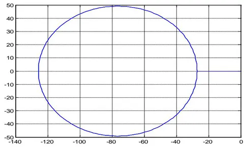
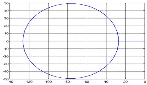
d) Regions of Absolute Stability

For case one: The stability polynomial for half step with three off step point gives

Stability Region for Case Two For case two:

The stability polynomial for half step with three offstep point gives

Stability Region for Case One

e) Numerical Example

Problem I We consider a highly stiff problem

Exact Solution: $y(x)=\cos x,\quad h=\frac{1}{100}$

Notes

Table 1: Comparison of the proposed new half-step method with Adoghe & Omole (2019)

x-values	Error in case one of our method	Error in case two our method	Error in Adoghe & Omole 2019
0.01	6.100e-20	3.0000e-20	0.0000e+00
0.02	1.200e-19	6.0000e-20	1.1102e-16
0.03	1.900e-19	1.2000e-19	4.4409e-16
0.04	2.500e-19	1.6000e-19	5.8842e-15
0.05	3.200e-19	1.9000e-19	2.6201e-14
0.06	3.900e-19	2.5000e-19	8.3822e-14
0.07	4.500e-19	2.8000e-19	2.0750e-13
0.08	5.100e-19	3.2000e-19	4.4142e-13
0.09	5.600e-19	3.5000e-19	8.4743e-13
0.10	6.300e-19	4.0000e-19	1.5086e-12

Exact Solution: $y(x)=e^{-x}+xe^{-x},\quad h=\frac{1}{10}$

Table 2: Comparison of the proposed new half-step method with Mohammed & Adeniyi 2014

x-values	Error in case one of our method	Error in case two our method	Error in Mohammed & Adeniyi 2014
0.1	1.0434e-14	4.1832e-15	1.0000e-10
0.2	9.8731e-14	1.8599e-14	3.0000e-10
0.3	3.1317e-13	4.4245e-14	7.0000e-10
0.4	6.6668e-13	8.0431e-14	7.0000e-10
0.5	1.1507e-12	1.2552e-13	6.0000e-10
0.6	1.7445e-12	1.7743e-13	2.0000e-10
0.7	2.4220e-12	2.3395 e-13	9.0000e-10
0.8	3.1554e-12	2.9298e-13	2.8000e-09
0.9	3.9178e-12	3.5259e-13	5.4000e-09
1.0	4.6852e-12	4.1112e-13	3.5000e-09

Exact Solution: $y(x)=\frac{3}{16}(1-\cos2x)+\frac{x^{2}}{8}$ , $h=\frac{1}{10}$

Table 3: Comparison of the proposed new half-step method with Adebayo & Adebola (2016)

x-values	Error in case one of our method	Error in case two our method	Error in Adebayo &Adebola (2016)
0.1	7.9512e-14	3.1484e-14	2.970e-08
0.2	8.6717e-13	1.5843e-13	1.988e-07
0.3	3.1385e-12	4.2379e-13	6.508e-07
0.4	7.5504e-12	8.5820e-13	1.5480e-06
0.5	1.4585e-11	1.4765e-12	3.062e-06
0.6	2.4504e-11	2.2752e-12	5.3625e-06
0.7	3.7317e-11	3.2313e-12	8.6068e-06
0.8	5.2765e-11	4.3022e-12	1.2926e-05
0.9	7.0321e-11	5.4266e-12	1.8118e-05
1.0	8.9206e-11	6.5277e-12	2.5129e-05

Problem IV: $y'''=\exp(x)$ , $y(0)=3$ , $y'(0)=1$ , $y''(0)=5$ , $0\leq x\leq1$ .

Exact Solution:

Table 4: Comparison of the proposed new half-step method with Adeyeye & Omar (2018)

x-values	Error in case one of our method	Error in case two our method	Error in Adeyeye & Omar (2018)
0.1	1.70091e-15	4.54792e-15	6.34270e-13
0.2	1.91790e-14	3.06193e-14	2.32882e-12
0.3	7.25153e-14	9.80503e-14	5.44348e-12
0.4	1.83912e-13	2.28761-13	9.85317e-12
0.5	3.77884e-13	4.46995e-13	1.59974e-11
0.6	6.81541e-13	7.79496e-13	2.37223e-11
0.7	1.12480e-12	1.25594e-12	3.35679e-11
0.8	1.74091e-12	1.90890e-12	4.53443e-11
0.9	2.56633e-12	2.77460e-12	5.97084e-11
1.0	3.64152e-12	3.89290e-12	7.64322e-11

IV. CONCLUSIONS

It is evident from the above tables that our proposed new half-step third derivative hybrid block methods are converging faster than the existing method and can handle stiff problems.

Comparing the new method with the existing method respectively shows that the new half-step third derivative hybrid block method performs better on stiff and highly stiff problems than the existing method which is of high Order as compared to ours which is of Order four.