## I. INTRODUCTION Brazilian agriculture is recognized worldwide for its prominence in the global market, especially in producing grains and foods such as soybeans, corn, cotton, orange juice, cocoa, coffee, sugar, and meat (FAOSTAT, 2020). In recent years, the expansion of soybean cultivation in Brazil has intensified, consolidating the country as one of the world's leading exporters. This growth is due to the advance of new agricultural frontiers such as the MATOPIBA region, which covers parts of the frontiers of the states of Maranhão, Tocantins, Piauí, and Bahia, located predominantly in the Cerrado biome (Santos & Naval, 2022). Since the creation of the Brazilian Agricultural Research Corporation (EMBRAPA) in 1973, the knowledge generated by this institution has been fundamental in developing and adapting technologies for the tropical conditions of this type of production, especially in the Cerrado. This has boosted the development of the country's agricultural sector. These innovations have established Brazil as one of the largest global food producers and exporters (Nehring, 2016; Souza et al., 2020; EMBRAPA, 2024). However, despite the economic growth driven by the agricultural sector, this is one of the activities responsible for greenhouse gas (GHG) emissions, due to the use of fossil fuelbased fertilizers, the burning of biomass, the high density of cattle per unit area, and the use of heavy agricultural machinery, which also uses this type of fuel in its energy matrix (Liu et al., 2017). According to the Food and Agriculture Organization of the United Nations (FAO), the agricultural sector may be responsible for up to $21\%$ of the world's GHG emissions (FAO, 2016). The increase in the greenhouse effect can be exacerbated by the rising levels of carbon dioxide (CO2) in the atmosphere (Myhre et al., 2013), which is attributed to various causes. Agricultural production can contribute to this process through the actions described in the previous paragraph. However, paradoxically, plants play a crucial role in reducing these emissions through the biochemical phenomenon known as photosynthesis. During photosynthesis, plants capture CO2, solar energy, water, and nutrients from the soil, transforming them into organic matter and releasing oxygen as a byproduct. Because of this phenomenon, CO2 is often known as the gas of life. It can therefore be inferred that deforestation may be one of the primary causes of the reduced capacity to capture CO2, which is ultimately released by various sources (Felicio, 2014). Thus, one of the primary sources of CO2 emissions is the burning of fossil fuels (Forster et al., 2007). Additionally, land use changes can alter the flow of carbon dioxide (CO2), methane (CH4), and nitrous oxide (N2O)-greenhouse gases that result from modifications to biogeochemical processes (Forster et al., 2007; Houghton et al., 2012; Kirschbaum et al., 2012; Kim & Kirschbaum, 2015). Worldwide, it is estimated that approximately 420 million hectares of forest have been cleared since 1990. More than half (54%) of the world's forests are concentrated in just five countries: Russia, Brazil, Canada, the United States, and China. Meanwhile, agricultural land areas expanded by 6% between 2000 and 2021, contributing to a growth of 38% in permanent crops and 12% in temporary crops (FAO, 2020). In 2021, Brazil had 66 million hectares of arable land, with a $20\%$ increase in agricultural areas due to the expansion of temporary crops (FAO, 2023). It is, therefore, necessary to evaluate more rigorously how land is utilized as the main production factor in agriculture and its relationship with greenhouse gas emissions, given that it is directly related to changes in soil organic carbon stocks. This, in turn, is important for determining soil quality, natural fertility, agricultural productivity, and the fixation of atmospheric carbon dioxide $\left(\mathrm{CO}_{2}\right)$ (Kumar et al., 2022). In addition, the use of fire related to land use change can also reduce soil organic carbon stocks (Van der Werf et al., 2006; Van der Werf et al., 2010; Kim & Kirschbaum, 2015). 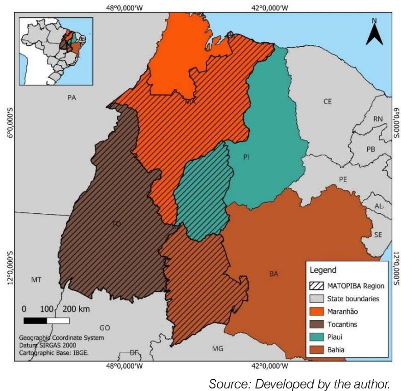In recent decades, since its implementation in the 1980s, the MATOPIBA agricultural frontier, which includes parts of the states of Maranhão (135 of its 217 municipalities), Tocantins (all 139 municipalities), Piauí (33 of its 224 municipalities), and Bahia (30 of its 417 municipalities on the frontier) (Figure 1), has emerged as one of the main regions for the expansion of grain production, especially soybeans.  Figure 1: Location Map of the MATOPIBA Region According to data from IBGE's Municipal Agricultural Production (PAM), in 2023 the 337 municipalities of MATOPIBA recorded a $9.6\%$ increase in cultivated area compared to the previous year. Consequently, production reached 18,943,144 tons, an increase of $11.2\%$, with an average yield of 3,581.94 kg/ha, representing a growth of $1.44\%$ compared to 2022. In addition, between 2013 and 2017, the GDP of agriculture in MATOPIBA reached R$17.1 billion, with an average annual growth rate of 7.7%(Souza, Magalhães & Castro, 2022). However, this economic growth has also had environmental impacts. Between 2010 and 2013, the MATOPIBA region was responsible for 45% of forest carbon emissions resulting from agricultural expansion in the Cerrado, with Maranhão making one of the largest contributions(14.42%)(Noojipady et al., 2017). the largest contributions (14.42%) (Noojipady et al., 2017). The conversion of native Cerrado areas into agricultural land intensifies deforestation (Rausch et al., 2019). In 2023, according to the Annual Report on Deforestation in Brazil, the MATOPIBA region was responsible for almost half $(47\%)$ of the loss of native vegetation in Brazil, with 858,952 hectares deforested, representing an increase of $59\%$ over the previous year. Of the 50 municipalities with the most deforestation in the country, 33 are in the Cerrado, and the 10 with the largest deforested areas are in this biome. The state of Maranhão led the national ranking, with 331,225 hectares deforested, an increase of $95.1\%$. The state of Tocantins experienced a $177.9\%$ increase in deforestation, with 230,253 hectares cleared, while Bahia deforested 290,606 hectares, representing a $27.5\%$ increase compared to 2022 (RAD, 2023). This change in land use, resulting from the conversion of native areas into agricultural land and pastures, drives deforestation and promotes the frequent use of fire (Reddington et al., 2015; Spera et al., 2016). According to data from MapBiomas Fogo, between 1985 and 2023, around 199.1 million hectares were burned in Brazil, of which $44.6\%$ (equivalent to 88.5 million hectares) were in the Cerrado biome, while the Amazon biome accounted for $19.6\%$ (MapBiomas Project, 2023). Although fire is a natural element used to clear areas where crops or pastures will be planted, it is becoming a threat due to its increasing frequency and the possibility of it getting out of control in the Cerrado due to agricultural expansion and deforestation. The Cerrado is responsible for $48\%$ of the country's soybean production and approximately a quarter of this production area is located in MATOPIBA (Pitta et al., 2017; Soterroni et al., 2019; Silva et al., 2021; MapBiomas Project, 2023). Given this scenario, studying the evolution of greenhouse gas (GHG) emissions and identifying the factors that likely contribute to the reduction or expansion of these emissions in the MATOPIBA region is essential for guiding public policies and investments that promote agriculture with lower or zero GHG emissions (Bezerra, 2022). Based on the above, this research aims to answer the following questions: 1 - How many municipalities in MATOPIBA had an increase or decrease in GHG emissions between 2006 and 2017? 2 - Which variables, and in what proportions, probably influenced these emissions in this time interval? To answer these questions, the general objective of this study is to investigate the factors that influence GHG emissions and reductions in agricultural production in the MATOPIBA region between 2006 and 2017. Specifically, the study seeks to: a - Ascertain the number of municipalities in the MATOPIBA region and, by state, identify which had an increase or decrease in GHG emissions between 2006 and 2017; b - Analyze the interaction between the variables tested in determining GHG emissions in this period; c - Evaluate how GHG emissions are influenced by the synergies between the indicators analyzed. ## II. MATERIAL AND METHODS ### a) Database and Construction of Indicators The research uses secondary data extracted from the 2006 and 2017 Agricultural Censuses, MapBiomas, NOAA (National Oceanic and Atmospheric Administration), and SEEG (System of Estimates of Greenhouse Gas Emissions and Removals), from which information was obtained on the variables that are supposed to affect greenhouse gas emissions in the municipalities of the MATOPIBA region over these 11 years. The variables and data sources used are shown in Table 1. Table 1: Variables that, by Hypothesis, Affect Greenhouse Gas (GHG) Emissions Positively (+) or Negatively (-) between 2006 and 2017 in MATOPIBA in this Research <table><tr><td>Variables</td><td>Hypothesis of the relation between Yi and Xij</td><td>Definition</td><td>Sources</td></tr><tr><td>Yi</td><td>GHG Emissions</td><td>(GHG2017/GHG2006) Emissions</td><td>Greenhouse Gas Emissions - SEEG (OC, 2022).</td></tr><tr><td>Xi1</td><td>(-)</td><td>(Municipal average annual rainfall2017) / (Municipal average annual rainfall2006)</td><td>NOAA (2022)</td></tr><tr><td>Xi2</td><td>(-)</td><td>(Vegetation cover) [(Crop areas + forest areas) / (total establishment area 2017)] / [(Crop areas + forest areas)/ (total establishment area 2006)]</td><td>Agricultural Censuses of 2006 and 2017 / IBGE</td></tr><tr><td>Xi3</td><td>(-)</td><td>[(Agricultural production value2017) / (Harvested agricultural area2017)] / [(Agricultural production value2006) / (Harvested agricultural area2006)]</td><td>Agricultural Censuses of 2006 and 2017 / IBGE</td></tr><tr><td>Xi4</td><td>(-)</td><td>[(Livestock production value2017) / (Pasture area2017)]/ [(Livestock production value2006) / (Pasture area2006)]</td><td>Agricultural Censuses of 2006 and 2017 / IBGE</td></tr><tr><td>Xi5</td><td>(-)</td><td>[(Recovered areas2017) / (Deforested areas2017)]/ [(Recovered areas2006) / (Deforested areas2006)]</td><td>MapBiomas</td></tr><tr><td>Xi6</td><td>(+)</td><td>[(Cattle quantity2017) / (pasture areas 2017)] / [(Cattle quantity2006) / (pasture areas 2006)]</td><td>Agricultural Censuses of 2006 and 2017 / IBGE</td></tr><tr><td>Xi7</td><td>(+)</td><td>[(Total tractors and machinery2017) / (total establishment area2017)] / [(Total tractors and machinery2006) / (total establishment area2006)]</td><td>Agricultural Censuses of 2006 and 2017 / IBGE</td></tr><tr><td>Xi8</td><td>(+)</td><td>[(Expenditure on agricultural pesticides2017) / (total area of municipal establishments 2017)] / [(Expenditure on agricultural pesticides2006) / (total area of municipal establishments 2006)]</td><td>Agricultural Censuses of 2006 and 2017 / IBGE</td></tr><tr><td>Xi9</td><td>(+)</td><td>[(Industrial sector GDP2017) / (Total municipal GDP2017)] / [(Industrial sector GDP2006) / (Total municipal GDP2006)]</td><td>Agricultural Censuses of 2006 and 2017 / IBGE</td></tr><tr><td>Xi10</td><td>(+)</td><td>CV rainfall 2017/ CV rainfall 2006</td><td>NOAA (2022)</td></tr><tr><td>Xi11</td><td>(+)</td><td>(Burn scars areas 2017 / Burn scars areas 2006)</td><td>MapBiomas</td></tr></table> The methodological approaches adopted to achieve the objectives of this research begin with the development of the indicators used. To assess changes in greenhouse gas (GHG) emissions between 2006 and 2017, in addition to the impact of the variables presented in Table 1 on these emissions, the indicators are constructed as follows: the relationship between the values observed in 2017 (final year) and those in 2006 (initial year) is estimated for both GHG emissions and the explanatory variables. This makes it possible to identify whether each variable increased or decreased over the period analyzed. In municipalities where the ratio between GEE2017 and GEE2006 is greater than 1, there has been an increase in emissions; if it is less than 1, there has been a reduction. The same process is applied to the explanatory or independent variables (Table 1). ### b) Methodology Adopted to Assess the First Research Objective To achieve the first objective of the research, we estimated the total number of municipalities where the ratios of GHG emissions in 2017 were higher than those observed in 2006. In these instances, the ratios are represented as Yi2017/Yi2006. Additionally, we measured the relationships between the variables believed to have influenced GHG emissions between 2006 and 2017, denoted as Xij2017/Xij2006. ### c) Methodology for Achieving the Second Objective To estimate the synergy between the variables that are thought to have influenced GHG emissions, Factor Analysis (FA) was used, using the principal component decomposition technique. Before using the principal component decomposition model, it was decided to transform all the variables into indices. The indices range from 1 to 100. In the case of the dependent variable, the ratio of GHG emissions between 2006 and 2017, the following procedure was adopted. The municipalities were ranked in descending order by the ratio of GHG emissions between 2006 and 2017. Therefore, the higher the value of this ratio, the higher the GHG emissions between 2006 and 2017. For this reason, the highest emissions value was assigned the index $= 100$. The other values were adjusted proportionally using a simple, straightforward rule of three. Thus, in the municipality where the GHG emissions index $= 100$, there was the highest emission of this gas between 2006 and 2017. In those municipalities where the GHG index is close to 1, this means that there was the greatest reduction in these emissions. About the 11 independent variables used to cause GHG emissions, the following criteria were adopted. All 5 variables whose hypothesis in this study establishes that they should cause a reduction in GHG emissions between 2006 and 2017 (GHG2017/2006 ≤ 1) were ranked in ascending order. The lowest value (worst case) is assigned an index of 100. The remaining values are adjusted proportionally using a simple inverse rule of three. These variables are marked with a (-) sign in Table 1 indicating that, by hypothesis, they cause a reduction in GHG emissions. The other 6 independent variables which, by hypothesis, should cause an increase in GHG emissions (GHG2017/2006) were ranked in descending order. The highest value of these variables (worst case) was assigned an index of 100. The other values are adjusted proportionally using a simple, direct rule of three. These variables are marked with a (+) sign in Table 1 indicating that, by hypothesis, they cause an increase in GHG emissions. ## i. Summary of the Factor Analysis Model as it Applies to the Study A summary of the factor analysis method applied in this study is presented below. In general, the factor analysis model can be expressed as follows: $$ \mathrm {X} = \mathrm {a f} + \mathrm {e} \tag {1} $$ In equation (1), $\mathsf{X} = (\mathsf{X}_1, \mathsf{X}_2, \dots, \mathsf{X}_p)^\top$ is a transposed vector of observable variables, while $\mathsf{f} = (\mathsf{f}_1, \mathsf{f}_2, \dots, \mathsf{f}_r)^\top$ represents a transposed vector consisting of r latent $(\mathsf{r} < \mathsf{p})$ factors that are not directly observable. The matrix $\mathbf{a}$ of coefficients has dimension $(\mathsf{p} \times \mathsf{r})$ of fixed coefficients, known as factor loadings; and $\mathsf{e} = (\mathsf{e}_1, \mathsf{e}_2, \dots, \mathsf{e}_r)^\top$ is a transposed vector of random terms. It is generally assumed that $E(\mathsf{e}) = E(\mathsf{f}) = 0$. At the outset, the estimated factor loadings may not be definitive; however, the factor analysis method enables the rotation of this initial structure for enhanced interpretation. In this study, varimax orthogonal rotation was used, which has the advantage of making the factors independent (Dillon & Goldstein, 1984; Johnson & Wichern, 1988; Basilevsky, 1994; Fávero et al., 2017). To construct the index, the factor scores are estimated after the orthogonal rotation of the initial structure. The factor score positions each observation in the space of common factors. Thus, for each factor fi, the i-th factor score that can be extracted is defined by Fi, and can be expressed as: $$ F _ {i} = b _ {1} X _ {i 1} + b _ {2} X _ {i 2} +.. + b _ {p} X _ {i p}; i = 1, 2,.., n; j = 1, 2.., p \tag {2} $$ Where $b_1, b_2, \ldots, b_p$ are regression coefficients; $X_{i1}, X_{i2}, \ldots, X_{ip}$ are "p" observable variables. Although $\mathrm{Fi}$ is not directly observable, it can be estimated using existing factor analysis techniques, using the matrix of observable variables $X$. Thus, equation (2) can be rewritten in a more compact form using matrix notation: $$ \mathrm{F}_{(nxq)} = \mathrm{X}_{(nxp)}.\mathrm{B}_{(pxq)} \tag{3} $$ In equations (2) and (3), the factor scores are influenced by the magnitude and units of the X variables. To avoid this problem, the X variables are normalized, resulting in: $$ Z_{ij} = \left[ \left(X_{i} - m_{xi}\right) / s_{xi}\right]; $$ Where $m_{\mathrm{xi}}$ is the mean of $X_{i}$, and $S_{\mathrm{xi}}$ is its standard deviation. Thus, equation (4) can be modified to: $$ \mathrm {F} _ {\left(\mathrm {n x q}\right)} = \mathrm {Z} _ {\left(\mathrm {n x p}\right)} \cdot \mathrm {b} _ {\left(\mathrm {p x q}\right)} \tag {5} $$ In equation (5), the vector "b" replaces "B", since the variables are already normalized. Pre-multiplying both sides of the equation by $(1/n)Z^{\top}$, where $n$ is the number of observations and $ZT$ is the transposed matrix of $Z$, gives us: $$ (1 / \mathrm {n}) Z ^ {\mathrm {T}} F = (1 / \mathrm {n}) Z ^ {\mathrm {T}} Z b. \tag {6} $$ The expression (1/n) $Z^{\mathrm{T}}Z$ corresponds to the correlation matrix of the X variables, called R. The matrix (1/n) $Z^{\mathrm{T}}F$ represents the correlation between the factor scores and the factors themselves, called L. The equation is redefined as: $$ \mathrm{L} = \mathrm{R}.\mathrm{b} $$ If R is a non-singular matrix, verified by the Bartlett test, the analysis can proceed. Thus, the hypothesis that the matrix of correlations between the variables is not an identity matrix must be rejected, with at least a $5\%$ error level (Favero, 2017). If $R$ is non-singular, multiply both sides of equation (7) by the inverse matrix of $R(R^1)$, resulting in: $$ \mathbf{b} = \mathrm{R}^{-}.\mathrm{L}. $$ For the estimated model to be statistically valid, it is essential to conduct the Kaiser-MeyerOlkin (KMO) test, which should yield a value greater than 0.5. Additionally, the total variance explained by the orthogonal factors must exceed $50\%$ (Hair et al., 2005; Maroco, 2003; Favero, 2017). After determining the "b" vector (as shown in equation 8), the compositions of each estimated factor are identified based on the magnitudes of the factor loadings. The factors, which are a reduction of the original variables $(k < n)$, can be redefined and renamed according to the magnitudes of the factor loadings that each variable presents in each component factor. The principal component decomposition process permits the generation of factor scores. These factor scores, represented by FE, are normalized variables with a mean of zero and a standard deviation of one. Positive and negative values gravitate around this zero mean FE. These factor scores can be converted into partial indices associated with each municipality (li) using equation (9). These partial indices can be supplemented, depending on the variables grouped in the composition of each factor score that generated it. $$ I_{i} = \left(FE_{i} - FE_{MN}\right) / \left(FE_{MX} - FE_{MN}\right) \\tag{9} $$ In equation (9), FEi is the i-th normalized factor score, FEMN is the minimum value of the factor score, and FEMX is the maximum value. In this manner, the li indices will range between zero and one, and they will be utilized in this study to identify the expected results for the second objective. The relationship between GHG emissions and the partial indices (I1; I2,..., Ip) can be described by the following equation: $$ \mathrm {G H G} _ {\mathrm {i}} = \mathrm {f} \left(\mathrm {I} _ {1}; \mathrm {I} _ {2}, \dots , \mathrm {I} _ {\mathrm {p}}\right) \tag {10} $$ This equation summarizes how the indices derived from the factor scores explain the variation in GHG emissions in the different municipalities. ## ii. Methodology Adopted to Achieve the Third Objective To achieve the third objective of this research, the Artificial Neural Networks (ANN) model was used to investigate how GHG emissions are influenced by the synergy of partial indices $(l_{1}, l_{2}, \dots, l_{p})$. ANNs are part of computational artificial intelligence. One of the main areas of application of ANNs is in the prediction of multivariate statistical data that is both nonlinear and non-parametric (Sharda & Patil, 1992; Lee et al., 2017). Zhang et al (1998) report that one of the procedures of computational artificial intelligence normally used to predict time series is the training of ANNs, based on the architecture and learning of the human brain. In this way, according to Zhang et al (1998), ANNs work like the human brain, seeking to recognize regularities and patterns in data, being able to learn from experience, and make generalizations based on previously accumulated knowledge. ANNs are nonlinear models, unlike traditional forecasting models such as Box & Jenkins (1976) and Pankratz (1983), which assume that the series studied are generated by linear processes. When designing an ANN model, we can envision it as a network of artificial 'neurons' organized into layers. The variables used to predict (inputs) a dependent variable (output) form the lower layer, while the predicted variables form the upper layer. The ANN model also allows for the possibility of intermediate layers, generally known as hidden layers (Sharda & Patil, 1992). Designed to represent how the human brain processes information, ANNs are computer algorithms that add knowledge by detecting patterns and correlations and can be trained through experience. They consist of hundreds of artificial neurons (or nodes) interconnected in hierarchical layers. Each neuron has a specific output function and the connection between each two nodes has a weight, constituting its artificial neural network memory. It is through these weights that the power of neural computations is reflected, i.e. the degree of influence that one cell exerts on another. Built to simulate the biological function of a neuron, each node has weighted inputs, a transfer function, and an output. Feedforward neural networks linearly transmit information, from the input layer to the output layer, and are among the most popular types used in various applications (Figure 1) (Agatonovic-Kustrin; Beresford, 2000; Gomez, Fernandez & Peñauela, 2021). In this research, the process begins with data entry, in which the explanatory variables correspond to the partial indices generated by factor analysis, and the dependent variable is represented by GHG emissions (Yi). The data was randomly divided into two sets: $70\%$ was used to train the model and $30\%$ was reserved for the test set (Liu &Cocea, 2017; Dao et al., 2020). The output of a neuron can be written mathematically: $$ \mathrm {Y i} = \mathrm {f} (\mathrm {n}) \tag {12} $$ Where $n$ is the weighted sum of the input signals plus an adjustment term (bias), defined as: $n =$ $$ n = \sum_ {i = 1} ^ {p} \left(w _ {j} \cdot X _ {j}\right) + b \tag {13} $$ Where $\mathrm{Xi}_1, \mathrm{Xi}_2, \dots, \mathrm{Xi}_p$ are the neuron's input signals (partial indices generated by factor analysis); $w_1, w_2, \dots, w_p$ are the weights associated with each input, determining the importance of each signal in the process; "b" is the bias term, used to adjust the flexibility of the model; and $f(\star)$ is the activation function, responsible for the non-linearity of the model, enabling the network to learn complex relationships between the data. The model's performance was assessed using quantitative metrics, including the Root Mean Square Error (RMSE), the Mean Absolute Error (MAE), and the Mean Absolute Percentage Error (MAPE). The lower the estimated values for these measurements, the better the adjustments. The RMSE is calculated by the root mean square difference between the predicted and observed values, shown in Equation 14. It provides an overview of the model's accuracy. The lower the RMSE, the more accurate the model. The Mean Absolute Error (MAE), as measured by equation (15), is also a metric used for evaluating models. Finally, the Mean Absolute Percentage Error (MAPE), as measured by equation (16), expresses errors as a percentage, making it easier to interpret the observed values (Pham et al., 2018; Elsaraiti, 2024). Using several metrics is advantageous for obtaining a broader view of the model's performance from different perspectives (Tripathy & Prusty, 2021). $$ \mathrm{R M S E} = \sqrt{\frac{1}{n} \sum_ {i = 1} ^ {n} \left(v _ {\text{observed}} - v _ {\text{predicted}}\right) ^ {2}} \tag{14} $$ $$ \mathrm{M A E} = \frac{1}{n} \sum_ {i = 1} ^ {n} | v _ {\text{observed}} - v _ {\text{predicted}} | \tag{15} $$ $$ \mathrm{MAPE} = \frac{1}{n} \sum_{i=1}^{n} \left| \frac{v_{\text{observed}} - v_{\text{predicted}}}{v_{\text{predicted}}} \right| * 100 \tag{16} $$ ## III. RESULTS AND DISCUSSION To enhance the clarity of the presentation and discussion of the results, they have been organized according to the timeline of the research objectives. ### a) Results Found for the First Objective Table 3 and Figure 2 show the absolute and relative frequencies of the MATOPIBA municipalities for states that showed an increase or decrease in GHG emissions between 2006 and 2017. Table 3: Absolute and Relative Frequencies of GHG Missions in MATOPIBA Municipalities from 2006 to 2017 <table><tr><td>States</td><td>Absolute frequencies of municipalities where the ratio of GHG emissions between 2017</td><td>Relative Frequency (%)</td><td>Absolute frequencies of municipalities where the ratio of GHG emissions between 2017</td><td>Relative Frequency (%)</td></tr><tr><td></td><td>and 2006 was less than 1 (GHG &lt; 1)</td><td></td><td>and 2006 was greater than 1 (GHG &gt;1)</td><td></td></tr><tr><td>Maranhão</td><td>50</td><td>37</td><td>85</td><td>63</td></tr><tr><td>Tocantins</td><td>33</td><td>23,7</td><td>106</td><td>76,3</td></tr><tr><td>Piauí</td><td>8</td><td>24,2</td><td>25</td><td>75,8</td></tr><tr><td>Bahia</td><td>9</td><td>30</td><td>21</td><td>70</td></tr><tr><td>Total</td><td>100</td><td>100</td><td>237</td><td>100</td></tr></table>  Figure 2: 2017/2006 GHG Ratio for the MATOPIBA Region Source: Based on the survey result. Legend - Municipalities assessed where the proportion of greenhouse gas (GHG) emissions between 2006 and 2017 was below one - Municipalities assessed where the proportion of greenhouse gas (GHG) emissions between 2006 and 2017 was above one - Municipal Limits - State Limit - Brazil There was a predominance of municipalities with an increase in GHG emissions during the analyzed period. Of the 337 municipalities in the MATOPIBA region, 237 (approximately $70.3\%$ ) experienced an increase in emissions, while 100 ( $29.7\%$ ) reported a reduction. Among the municipalities in the state of Maranhão, 50 out of a total of 135 ( $37\%$ ) experienced a reduction in emissions, while 85 ( $63\%$ ) reported an increase. In Tocantins, of the 139 municipalities, 33 ( $23.7\%$ ) registered a decrease in emissions, while 106 ( $76.3\%$ ) showed an increase. In Piauí, out of 33 municipalities, only 8 (24.2%) reduced emissions, while 25 (75.8%) experienced an increase. In the state of Bahia, out of a total of 30 municipalities in MATOPIBA, 9 (30%) reduced emissions, while 21 (70%) showed an increase (Table 3). ### b) Results Obtained for the Second Objective Table 4 presents the results obtained from the principal component decomposition procedure of the factor analysis (FA) conducted in this research. Table 4: Results Found Showing the Decomposition of the 11 Original Variables into 3 Main Components <table><tr><td></td><td></td><td colspan="3">Rotated components Matrix</td><td colspan="3">Component Score Coefficient Matrix</td></tr><tr><td>Variables</td><td></td><td>1</td><td>2</td><td>3</td><td>1</td><td>2</td><td>3</td></tr><tr><td>Index of rainfall</td><td>Xi1</td><td>0.000</td><td>0.009</td><td>1.000</td><td>-0.001</td><td>-0.003</td><td>0.500</td></tr><tr><td>Index of vegetation cover</td><td>Xi2</td><td>-0.296</td><td>0.856</td><td>-0.006</td><td>0.036</td><td>0.281</td><td>-0.008</td></tr><tr><td>Index of agricultural production value</td><td>Xi3</td><td>-0.225</td><td>0.896</td><td>0.013</td><td>0.061</td><td>0.306</td><td>0.001</td></tr><tr><td>Index of relative livestock value</td><td>Xi4</td><td>-0.035</td><td>0.788</td><td>0.008</td><td>0.098</td><td>0.291</td><td>-0.001</td></tr><tr><td>Index of rLative recovered areas</td><td>Xi5</td><td>-0.264</td><td>0.941</td><td>0.009</td><td>0.056</td><td>0.317</td><td>-0.001</td></tr><tr><td>Index or relative cattle quantity</td><td>Xi6</td><td>0.927</td><td>-0.260</td><td>-0.009</td><td>0.219</td><td>0.029</td><td>-0.004</td></tr><tr><td>Index of _relative_machinery</td><td>Xi7</td><td>0.947</td><td>-0.170</td><td>-0.024</td><td>0.237</td><td>0.066</td><td>-0.013</td></tr><tr><td>Index of relative expenditure in pesticides</td><td>Xi8</td><td>0.865</td><td>-0.258</td><td>0.013</td><td>0.202</td><td>0.021</td><td>0.007</td></tr><tr><td>Index of relative industrial GNP</td><td>Xi9</td><td>0.927</td><td>-0.083</td><td>-0.001</td><td>0.243</td><td>0.096</td><td>-0.002</td></tr><tr><td>Index of relative cv rainfall</td><td>Xi10</td><td>0.000</td><td>0.009</td><td>1.000</td><td>-0.001</td><td>-0.003</td><td>0.500</td></tr><tr><td>Index of relative Burn scars areas</td><td>Xi11</td><td>0.937</td><td>-0.199</td><td>0.020</td><td>0.230</td><td>0.053</td><td>0.010</td></tr><tr><td>Kaiser-Meyer-Olkin Measure of Sampling Adequacy:</td><td></td><td></td><td></td><td></td><td></td><td></td><td>0.738</td></tr><tr><td>Bartlett's Test of Sphericity</td><td></td><td></td><td></td><td></td><td></td><td></td><td></td></tr><tr><td>Approx. Chi-Square</td><td></td><td></td><td></td><td></td><td></td><td></td><td>8186.72</td></tr><tr><td>Degrees of Freedom</td><td></td><td></td><td></td><td></td><td></td><td></td><td>7</td></tr><tr><td>Significance level.</td><td></td><td></td><td></td><td></td><td></td><td></td><td>0.000</td></tr><tr><td>Total Variance Explained (%)</td><td></td><td></td><td></td><td></td><td></td><td></td><td>88.232</td></tr><tr><td>Variance Explained by Component 1 (%)</td><td></td><td></td><td></td><td></td><td></td><td></td><td>40.464</td></tr><tr><td>Variance Explained by Component 2 (%)</td><td></td><td></td><td></td><td></td><td></td><td></td><td>29.575</td></tr><tr><td>Variance Explained by Component 3 (%)</td><td></td><td></td><td></td><td></td><td></td><td></td><td>18.193</td></tr></table> Observations: Extraction Method: Principal Component Analysis; Rotation Method: Varimax with Kaiser Normalization. Component Scores. Rotation converged in 4 iterations. The evidence presented in Table 4 indicates that the adjustment obtained using the principal component decomposition (PCD) method was statistically significant. The Bartlett test, which yielded a high level of significance $(p = 0.00)$, demonstrated that the correlation matrix of the independent variables is not an identity matrix. The estimated statistic for the Kaiser-Meyer-Olkin Measure of Sampling Adequacy (KMO) test was 0.738, and the total variance explained by the adjusted model was approximately $88.232\%$. The variances explained by each estimated component after Varimax orthogonal rotation were $40.464\%$, $19.373\%$, and $18.137\%$, respectively, for components 1, 2, and 3. These results indicate that the greatest synergy captured by the DCP procedure was in component 1, which measures the ratios of: the number of cattle per hectare; the number of tractors and machinery; spending on pesticides; and industrial GDP about the total GDP of the municipalities; and the evolution of burn scars in the period studied. All these variables captured in this component, as assumed in this research, must have positively affected greenhouse gas emissions between 2006 and 2017. This synergy, as we have seen, is responsible for explaining $40.464\%$ of the total explanatory capacity of the model generated (Table 4). From the results shown in Table 4, it can also be seen that associated with the second component generated in the research, whose variance explains approximately $29.575\%$ of the total explained variance, are four of the five variables that are supposed to cause a reduction in greenhouse gas emissions: the vegetation cover index; the index that measures the productive potential of crops; the index that measures the productive capacity of animal husbandry and the index that measures the recovery of degraded areas. For the third component, the greatest synergies were between the variables rainfall index, which is supposed to reduce GHG emissions, and the index measuring rainfall instability, as measured by the coefficients of variation, which is supposed to increase GHG emissions. These two variables account for $18.193\%$ of the total explained variance. Based on these results, the matrix was generated, which is made up of 3 factor scores that capture these synergies (Table 4). ### c) Results Obtained for the Third Objective As shown above, the third objective of this research sought to assess how GHG emissions are influenced by the synergies between the indicators analyzed. To do this, the GHG emissions ratios between 2006 and 2017 were transformed into indices. In the previous step, when using FA, it was assumed that the relationships between the variables were linear. Thus, the three estimated factor scores are linearly independent. In this step, it is assumed that the relationship between the GHG emissions index between 2006 and 2017 and the independent variables transformed into factor scores is non-linear. The artificial neural network (ANN) model is used to perform the test. The results are shown in Table 5 and Figure 3. Table 5: Estimation results using ANN, with the GHG emissions index as the dependent variable and the FS1, FS2 and FS3 indices as independent variables <table><tr><td colspan="3">GHG2017/2006 emissions ≤ 1</td><td colspan="3">GHG2017/2006 emissions &gt;1</td></tr><tr><td colspan="2">Relative error in the Training period (%)</td><td>1.011</td><td colspan="2">Relative error in the Training period (%)</td><td>1.002</td></tr><tr><td colspan="2">Relative error in the Testing period (%)</td><td>0.908</td><td colspan="2">Relative error in the Testing period (%)</td><td>0.997</td></tr><tr><td colspan="2">Number of Units in Hidden Layer including 1 bias Hiden Layer</td><td>3</td><td colspan="2">Number of Units in Hidden Layer including 1 bias Hiden Layer</td><td>4</td></tr><tr><td colspan="3">Independent Variable Importance</td><td colspan="3">Independent Variable Importance</td></tr><tr><td>Variabels</td><td colspan="2">Importance (weights)</td><td>Variabels</td><td colspan="2">Importance (weights)</td></tr><tr><td>FS1</td><td colspan="2">0.276</td><td>FS1</td><td colspan="2">0.486</td></tr><tr><td>FS2</td><td colspan="2">0.496</td><td>FS2</td><td colspan="2">0.391</td></tr><tr><td>FS3</td><td colspan="2">0.228</td><td>FS3</td><td colspan="2">0.123</td></tr><tr><td colspan="3">Acuracy tests</td><td colspan="3">Acuracy tests</td></tr><tr><td>RMSE</td><td colspan="2">3.12</td><td>RMSE</td><td colspan="2">10.49</td></tr><tr><td>MAE</td><td colspan="2">2.52</td><td>MAE</td><td colspan="2">6.58</td></tr><tr><td>MAPE</td><td colspan="2">13.11</td><td>MAPE</td><td colspan="2">21.29</td></tr></table> The results presented in Table 5 and Figure 3 show that, in the 100 municipalities where there was a reduction in GHG emissions between 2006 and 2017, the score of the factor that brings together the four variables (FS2) that hypothetically impact this reduction had the highest weight (0.496), followed by the score of FS2, bringing together the variables that, by hypothesis, contributed to the increase in GHG emissions between 2006 and 2017, with a weight of 0.276. Meanwhile, FS3, which brings together the variables associated with rainfall and instability, weighted 0.228. Among the six variables transformed into indices, which were hypothesized to contribute to the increase in GHG emissions between 2006 and 2017, five were grouped into score factor 1 (SF1), with an estimated weight of 0.486. Factor score 2 (FS2) had a weight of 0.391 in this definition, while factor score 3 (FS3) had a weight of 0.123 (see Table 5 and Figure 3). These results prove the hypotheses of this research, indicating that the variables that were supposed to cause a reduction and increase in GHG emissions between 2006 and 2017 in Matopiba. It can also be seen that the prediction errors in both the training and testing phases were quite low. In addition, the RMSE, MAE, and MAPE tests also showed very low values, thus confirming the accuracy of the adjustments.  Figure 3: Relative importance of each factor score in Matopiba municipalities with GHG emissions $\leq$ and GHG emissions $>1$ Sources: Results found in the search As shown in the evidence presented in Table 5, to estimate the weights associated with each of the independent (explanatory) variables in the group of 100 MATOPIBA municipalities where the GHG ratio $\leq 1$, the ANN model used 3 Units in Hidden Layer, including 1 Hiden Layer bias. To estimate the importance of the explanatory variables in municipalities where the GHG ratio $>1$, the model used 4 Units in the Hidden Layer, including 1 Hiden Layer bias. In municipalities where GHG emissions are less than or equal to 1, the highest weight was estimated for variable FS2 (0.480), followed by FS3 (0.286), and the lowest weight was associated with the independent variable FS1 (0.234). These results highlight the significance of all the original variables synthesized in FS2, as they are expected to contribute to reducing greenhouse gas emissions. Therefore, the research hypothesis is confirmed. About the estimated weights for the variables constructed linearly for the municipalities in which the GHG ratios $>1$, it can be seen that, as expected, the greatest weighting was given to the FS1 combination (0.629), which synergistically brings together practically all the original variables that are assumed in this research to have contributed to the increase in greenhouse gas emissions between 2006 and 2017. It can be seen that the rainfall ratios, as well as the rainfall instability ratios measured by the coefficients of variation, both contributed to a reduction and an increase in GHG emissions. ## IV. CONCLUSIONS From the results of the evidence extracted from the research, it was shown that of the 327 municipalities that are part of the MATOPIBA agricultural frontier region, 100 experienced a reduction in GHG emissions between 2006 and 2017, the period in which this research was carried out. In the remaining 237 municipalities, GHG emissions increased over the same period. We tested 5 variables that were assumed to have led to a reduction in GHG emissions in the period under investigation and 6 variables that were assumed to have led to an increase in emissions. The methodological procedures used in this research are unprecedented in this type of study, in that it uses two models in sequence. This study employed a model that assesses linear relationships through factor analysis using the principal component decomposition technique. In this process, the 11 observed variables were reduced to three unobserved variables, referred to as factor scores. These factor scores are orthogonal and linearly independent. In the second methodological stage, the relationships were estimated between the dependent variable that measures GHG emissions between 2006 and 2017 and the three-factor scores in which the 11 original independent variables were synthesized by synergy. At this stage, it was assumed that the relationships were non-linear. Therefore, artificial neural networks (ANN) were employed to evaluate the weights that each of the three factor scores contributes to explaining the dependent variable. It was observed that the assumptions made for this research were confirmed. Of the five variables hypothesized to contribute to a reduction in GHG emissions, four were grouped together in one of the factor scores and had the highest weighting in explaining greenhouse gas emissions in the MATOPIBA municipalities that experienced a decline in GHG emissions between 2006 and 2017. On the other hand, of the 6 variables that were tested and assumed to have led to an increase in greenhouse gas emissions between the two periods, 5 were brought together in synergy in another factor score (unobserved variable generated by the linear procedure) and had the highest weighting in the municipalities that had an increase in GHG emissions between 2006 and 2017. Thus, the results of this research can indicate the paths that should be followed in agricultural practices on this agricultural frontier. Furthermore, they can guide future studies by identifying which variables may contribute to the emission or reduction of GHG emissions. The overall conclusion of this research is that the two questions motivating its execution were answered, and the proposed objectives were achieved. The municipalities in the MATOPIBA region that increased and decreased GHG emissions between 2006 and 2017 were identified, along with the variables and their respective weightings that influenced these changes in emissions.

Generating HTML Viewer...

References

45 Cites in Article
S Agatonovic-Kustrin,R Beresford (2000). Basic concepts of artificial neural network (ANN) modeling and its application in pharmaceutical research.
F Bezerra (2022). Evaluation of low carbon emission and climate-smart agriculture in Brazil.
G Box,G Jenkins (1976). Time series analysis: Forecasting and control.
Dong Dao,Hojjat Adeli,Hai-Bang Ly,Lu Le,Vuong Le,Tien-Thinh Le,Binh Pham (2020). A Sensitivity and Robustness Analysis of GPR and ANN for High-Performance Concrete Compressive Strength Prediction Using a Monte Carlo Simulation.
M Elsaraiti (2024). Short-term power consumption forecasting using neural networks with first-and second-order differencing.
Gustavo Braga,Giovana Maciel,Allan Ramos,Marcelo Carvalho,Francisco Fernandes,Liana Jank (2024). Dry matter yield of promising Panicum maximum genotypes in response to phosphorus and lime on Brazilian savanna.
Ricardo Felício (2014). MUDANÇAS CLIMÁTICAS” E “AQUECIMENTO GLOBAL” – NOVA FORMATAÇÃO E PARADIGMA PARA O PENSAMENTO CONTEMPORÂNEO?.
(2010). Climatesmart" agriculture: Policies, practices and financing for food security, adaptation and mitigation.
(2013). The Imels-FAO project “International Alliance on Climate-Smart Agriculture”.
Mechlem Kerstin (2016). Food and Agriculture Organization of the United Nations (FAO).
(2020). Global Forest Resources Assessment 2020.
(2023). Food and Agriculture Organization of the United Nations (FAO).
(2023). Land statistics and indicators 2000–2021.
Mechlem Kerstin (2024). Food and Agriculture Organization of the United Nations (FAO).
P Forster (2007). Changes in atmospheric constituents and in radiative forcing.
I Miranda,J Jaramillo,G Peñuela (2021). Hybrid multivariate statistical and neural network model to predict greenhouse gas emissions.
R Houghton (2012). Emissões de carbono do uso da terra e mudançanacobertura da terra.
D.-G Kim,M Kirschbaum (2015). The effect of land-use change on the net exchange rates of greenhouse gases: A compilation of estimates.
M Kirschbaum (2012). Comprehensive evaluation of the climate-change implications of shifting land use between forest and grassland: New Zealand as a case study.
Sandeep Kumar,Ram Meena,Seema Sheoran,Chetan Jangir,Manoj Jhariya,Arnab Banerjee,Abhishek Raj (2022). Remote sensing for agriculture and resource management.
J Lee (2017). Deep learning in medical imaging: General overview.
Han Liu,Mihaela Cocea (2017). Semi-random partitioning of data into training and test sets in granular computing context.
Xuyi Liu,Shun Zhang,Junghan Bae (2017). The nexus of renewable energy-agriculture-environment in BRICS.
G Myhre (2014). Anthropogenic and Natural Radiative Forcing.
R Nehring (2016). Yield of dreams: Marching west and the politics of scientific knowledge in the Brazilian Agricultural Research Corporation (Embrapa).
Praveen Noojipady,C Morton,N Macedo,C Victoria,Chengquan Huang,K Gibbs,L Bolfe (2017). Forest carbon emissions from cropland expansion in the Brazilian Cerrado biome.
Alan Pankratz (1983). Forecasting with Univariate Box‐Jenkins Models.
Binh Pham,Le Son,Tuan-Anh Hoang,Duc-Manh Nguyen,Dieu Tien Bui (2018). Prediction of shear strength of soft soil using machine learning methods.
Projetomapbiomas (2024). Mapeamento das áreasqueimadas no Brasil entre 1985 a 2023 -Coleção 3.
F Pitta,G Vega (2017). Impacts of agribusiness expansion in the MATOPIBA region: Communities and the environment.
Mapbiomas (2024). RAD 2023: RelatórioAnual do Desmatamento no Brasil 2023.
Lisa Rausch,Holly Gibbs,Ian Schelly,Amintas Brandão,Douglas Morton,Arnaldo Filho,Bernardo Strassburg,Nathalie Walker,Praveen Noojipady,Paulo Barreto,Daniel Meyer (2019). Soy expansion in Brazil's Cerrado.
C Reddington,E Butt,D Ridley,P Artaxo,W Morgan,H Coe,D Spracklen (2015). Air quality and human health improvements from reductions in deforestation-related fire in Brazil.
J Santos,L Naval (2022). Soy water footprint and socioeconomic development: An analysis in the new agricultural expansion areas of the Brazilian cerrado (Brazilian savanna).
Ramesh Sharda,Rajendra Patil (1992). Connectionist approach to time series prediction: an empirical test.
P Silva (2021). Putting fire on the map of Brazilian savanna ecoregions.
Brian Sims,Josef Kienzle (2017). Sustainable Agricultural Mechanization for Smallholders: What Is It and How Can We Implement It?.
G Souza,E Gomes,E Alves,J Gasques (2020). Technological progress in Brazilian agriculture.
D Souza,De,L Magalhães,G Castro (2022). Uma avaliação do impacto do crédito rural e do mercado de trabalho à agropecuária do Matopiba.
S Spera,G Galford,M Coe,M Macedo,J Mustard (2016). Land-use change affects water recycling in Brazil's last agricultural frontier.
Debesh Tripathy,B Prusty (2021). Forecasting of renewable generation for applications in smart grid power systems.
G Van Der Werf (2010). Global fire emissions and the contribution of deforestation, savanna, forest, agricultural, and peat fires (1997-2009).
G Van Der Werf,J Randerson,L Giglio,G Collatz,P Kasibhatla,A Arellano (2006). Interannual variability in global biomass burning emissions from 1997 to 2004.
Guoqiang Zhang,B Eddy Patuwo,Michael Y. Hu (1998). Forecasting with artificial neural networks:.
No ethics committee approval was required for this article type.
Data Availability
Not applicable for this article.
How to Cite This Article
José de Jesus Sousa Lemos. 2026. \u201cHybrid Model of Artificial Neural Networks and Principal Component Decomposition for Predicting Greenhouse Gas Emissions in the Brazilian MATOPIBA Region\u201d. Global Journal of Human-Social Science - E: Economics GJHSS-E Volume 25 (GJHSS Volume 25 Issue E1): .
Explore published articles in an immersive Augmented Reality environment. Our platform converts research papers into interactive 3D books, allowing readers to view and interact with content using AR and VR compatible devices.
Your published article is automatically converted into a realistic 3D book. Flip through pages and read research papers in a more engaging and interactive format.
Greenhouse gas (GHG) emissions in agricultural production represent a global environmental challenge, and it is necessary to understand the factors that influence them to develop sustainable practices. The general objective of this research is to investigate some of the factors that probably influence GHG emissions and reductions in agricultural production in the MATOPIBA region of Brazil between 2006 and 2017. A hybrid methodology was used, and the first stage used linear models (decomposition into principal components) and non-linear models (artificial neural networks) to determine the relationships that should exist between the dependent variable (GHG emissions) and 11 variables. The data was obtained from the 2006 and 2017 Brazilian Agricultural Census, MapBiomas, SEEG, and NOAA. The results showed that of the 373 municipalities that make up MATOPIBA, only 100 did not see an increase in GHG emissions between 2006 and 2017. The principal component decomposition method reduced the 11 initial variables into 3 orthogonal and unobserved variables. In one of the unobserved variables, 4 of the five variables that are supposed to cause a reduction in GHG emissions were brought together. The 5 variables thought to have caused an increase in GHG emissions were condensed into 5.
Our website is actively being updated, and changes may occur frequently. Please clear your browser cache if needed. For feedback or error reporting, please email [email protected]
Thank you for connecting with us. We will respond to you shortly.
Lorem ipsum dolor sit amet, consectetur adipiscing elit. Ut elit tellus, luctus nec ullamcorper mattis, pulvinar dapibus leo.
Hybrid Model of Artificial Neural Networks and Principal Component Decomposition for Predicting Greenhouse Gas Emissions in the Brazilian MATOPIBA Region