I. INTRODUCTION

In recent years, there has been a noticeable increase in the severity of droughts in central Europe and various other regions around the world (Balting et al. (2021), Satoh et al. (2022)). These prolonged periods of water scarcity have had significant impacts on the natural water cycle and the ecosystems that rely on it (Trumbore et al. (2015), Neumann et al. (2017), Senf et al. (2020)). As a result, addressing this issue requires a comprehensive reevaluation of our approach to forest and landscape design (Liu et al. (2022), Gvein et al. (2023)), along with the implementation of appropriate hydrological methods. Isotope-based hydrograph separations can be particularly helpful in this regard, as they can provide insights into the travel times of water within the catchment.

Over the past few decades, the separation of storm hydrographs using stable isotope tracers has become a standard method for investigating runoff generation processes in catchment hydrology. The early pioneering work was accomplished in the late 1960s and 1970s (Pinder and Jones (1969), Dincer et al. (1970), Martinec et al. (1974), and Fritz et al. (1976), Sklash and

Farvolden (1979)), and over the years, the methodology has been progressively expanded and adapted to address the challenges and tasks found in the feld (Klaus and McDonnell (2013), Jasechko (2019)). Hoeg (2019) recently proposed a method that iteratively extends the standard two-component separation, such that $n$ time components are separated by using a single stable isotope tracer. This approach can be used to trace the event water over a much longer period after the initial event, hence expanding the space of addressable use cases for catchment hydrologists. Hoeg (2019) applied the new method to an experimental data set of the mountainous Zastler catchment $(18.4{\mathrm{km}}^2$, Southern Black Forest, Germany) and compared the outcome with previous investigations in that area, showing the influence of antecedent moisture conditions on the event water contributions of subsequent events. This iterative extension uncovered the temporal structure of the pre-event component, and enabled a closer look at the temporal composition of the pre-event water, hence determining the extent to which recent events were involved.

A catchment response pattern related to antecedent moisture conditions similar to that of the Zastler catchment was found by Iorgulescu et al. (2007); they used a hydrochemical model based on a parameterization of three runoff components (direct precipitation, acid soil water, and deep groundwater) to predict conservative tracer data in the Haute-Mentue catchment (12.5 ${\mathrm{km}}^2$, Swiss Plateau). The authors concluded that the soil water component that corresponds to recent water stored in the upper soil horizons dominates catchment outflow in wet conditions but is virtually absent in dry conditions. James and Roulet (2009) formulated antecedent moisture conditions and catchment morphology as controls on the spatial patterns of runoff generation. Based on stable isotopes, they examined the spatial patterns of storm runoff generation from eight small nested forest catchments ranging in size from 0.07 to $1.5{\mathrm{km}}^2$ (formerly the glaciated terrain of Mont Saint-Hilaire, Quebec), here as a function of antecedent moisture conditions and catchment morphology. For the storms observed under dry conditions, larger magnitudes of new water were generated from the three largest catchments attributable to basin morphology, while the storms observed under wet conditions exhibited no consistent pattern, with larger variability among the smaller catchments. The results illustrated the complexity of the influences of antecedent moisture conditions. For the pre-Alpine Erlenbach tributary $(0.7{\mathrm{km}}^2)$ Von Freyberg et al. (2018) showed that pre-event water as a fraction of precipitation was strongly correlated with all measures of antecedent wetness but not with storm characteristics, implying that wet conditions primarily facilitate the mobilization of old (pre-event) water rather than the fast transmission of new (event) water to streamflow, even at a catchment where runoff coefficients can be large.

Time series of the natural isotopic composition (2H, 18O) of precipitation and streamwater can provide important insights into ecohydrological phenomena at the catchment scale. However, multi-year, high-frequency isotope datasets are generally scarce, limiting our ability to study highly dynamic short-term ecohydrological processes. Von Freyberg et al. (2022) recently presented a four years of daily isotope measurements in streamwater and precipitation at the Alp catchment in Switzerland and two of its tributaries. Therefore, the current study contributes here in three ways:

1. The classic hydrograph separation is embedded in a discretization of the catchment water and tracer mass balance along the event and pre-event time axis.

2. A characteristic seasonal variation of event, recent, and pre-recent runoff components is shown for the pre-Alpine Alp catchment (46.4 ${\mathrm{km}}^2$ ) and two smaller tributaries (Erlenbach, $0.7{\mathrm{km}}^2$, and Vogelbach, $1.6{\mathrm{km}}^2$ ).

3. Single rain-runoff events of the Erlenbach catchment are analyzed in more detail to visualize and quantify the rapid mobilization of recent water.

II. METHODS

a) Separation of n Time Components

Consider a control volume, for instance, a catchment in a river basin, with the following bulk water balance:

where $S$ is the time evolution of the water storage, $J$ is the precipitation, $ET$ is the evapotranspiration, and $Q$ is the total stream discharge. Let $C$ be a conservative isotope tracer with the following bulk mass balance:

where $C_{\mathrm{S}}$, $C_{\mathrm{J}}$, $C_{\mathrm{ET}}$, and $C_{\mathrm{Q}}$ are tracer concentrations of the water storage $S$, and the volumetric flow rates $J$, $ET$, and $Q$. In addition, there are the time points $t_0,t_1,\dots ,t_n$ and time intervals $[t_0,t_1[,[t_1,t_2[,\dots ,[t_{n-1},t_n[$ that describe the start and end of $n$ rainfall-runoff events along the time axis. Furthermore, there is a semantic time measure with the intervals $e$ (event) and $p$ (pre-event) that can be moved across the rainfall-runoff events, whereas the interval $p$ is the range of all intervals just before interval $e$. For instance, the stream discharge $Q$ during event $e$ is composed of water from the current rainfall-runoff event and the prior rainfall-runoff events, such that

where $C_{\mathrm{Q}}^e$ and $C_{\mathrm{Q}}^p$ are bulk tracer concentrations in the event and pre-event components, respectively. The same relations can be applied to the physical variables $\mathrm{d}S(t)/\mathrm{d}t$, $J(t)$, and $ET(t)$. Therefore, we can write generally for each volumetric flow rate $\dot{V}$ that

Furthermore, an iterative balance of the catchment event and pre-event mass and volume flows can be formulated along the time axis; that is, the pre-event water fraction of each rainfall-runoff event is entirely composed of the event water and pre-event water of the previous event. Therefore, for a first backward iteration, we have the following equations:

and for $\tau$ backward iterations, the whole system of the balance equations can be defined as follows:

Here, the event components ${\dot{V}}^e$, ${\dot{V}}^{e-1}$, ${\dot{V}}^{e-\tau }$ and pre-event components ${\dot{V}}^p$, ${\dot{V}}^{p-1}$, ${\dot{V}}^{p-\tau }$ are usually unknowns, whereas the volumetric flow rate $\dot{V}$ and its tracer concentration $C_{\dot{V}}$ are usually measured physical quantities. The tracer concentrations of the event components $C_{\dot{V}}^e$, $C_{\dot{V}}^{e-1}$, $\dots$, $C_{\dot{V}}^{e-\tau }$ and pre-event components $C_{\dot{V}}^p$, $C_{\dot{V}}^{p-1}$, $\dots$, $C_{\dot{V}}^{p-\tau }$ are usually the estimated physical quantities.

When being applied to all physical variables $\mathrm{d}S(t)/\mathrm{d}t$, $J(t)$, $ET(t)$, and $Q(t)$, the linear equation system (6) can be regarded as a discretization of the ordinary differential equation system (1) and (2) along $\tau +1$ rainfall events. In the literature, equation (3) is the standard two-component separation model and has been used in many hydrological investigations (Klaus and McDonnell (2013)). Sklash and Farvolden (1979) and Buttle (1994) mentioned the following criteria, which also apply to the iterative separation model (6):

1. The isotopic composition of the event component is significantly different from that of the pre-event component.

2. The event component maintains a constant isotopic signature in space and time, and if not, any variations can be accounted for.

3. The pre-event component maintains a constant isotopic signature in space and time, and if not, any variations can be accounted for.

I would like to add another criterion (Criterion 4) that is usually implicitly considered and demands that both the event water ${\dot{V}}^e$ and pre-event water ${\dot{V}}^p$ cannot be less than zero or larger than the total runoff $\dot{V}$ (Liu et al. (2004)). Given the equations above, this is the case if the tracer concentration in the volumetric flow $C_{\dot{V}}$ is always between that of the event water $C_{\dot{V}}^e$ and pre-event water $C_{\dot{V}}^p$. In the context of separation model (6), it is required for all the backward iterations $\tau$ that

Based on the measured knowns $\dot{V}$ and $C_{\dot{V}}$ and the estimated tracer concentrations $C_{\dot{V}}^e$, $C_{\dot{V}}^{e-1},\dots ,C_{\dot{V}}^{e-\tau }$ and $C_{\dot{V}}^p$, $C_{\dot{V}}^{p-1},\dots ,C_{\dot{V}}^{p-\tau }$, we can iteratively derive for $\tau \in \mathbb{N}$ backward iterations for the following solutions:

In addition, from linear equation system (6), we obtain the following total mass balance for each volumetric flow rate $\dot{V}$:

b) Determination of End Member Concentrations and Error Estimation

Resolving the system of balance equations being introduced in section 2.1 for the mentioned unknowns $({\dot{V}}^e,{\dot{V}}^{e-1}\dots {\dot{V}}^{e-\tau }$ and ${\dot{V}}^p$ ${\dot{V}}^{p-1}\dots {\dot{V}}^{p-\tau })$, also called end members, requires appropriate estimators for the end member concentrations $(C_{\dot{V}}^e,C_{\dot{V}}^{e-1},\dots ,C_{\dot{V}}^{e-\tau }$ and $C_{\dot{V}}^p,C_{\dot{V}}^{p-1},\dots ,C_{\dot{V}}^{p-\tau })$. For instance, when referring to the use case of hydrograph separations, which is addressed by the volumetric flow rate variable $Q$, the isotope signature $C_{\mathrm{J}}^e$ of precipitation $J$ can be taken as an estimator for the tracer concentration $C_{\mathrm{Q}}^e$ regarding end member $Q^e$, whereby changes in the isotope composition of precipitation as a result of evapotranspiration $ET$ or changes in the water storage $S$ (e.g. snow pack with sublimation and re-sublimation processes) must be considered. This context becomes visible if balance equations (1) and (2) are restricted to the event water fraction, such that

In a similar way, the isotope composition $C_{\mathrm{Q}}$ in the discharge $Q$, which occurs right before a rainfall-runoff event, can be taken as an estimator for the tracer concentration $C_{\mathrm{Q}}^p$ of the end member $Q^p$, whereby changes in the isotope composition of the bulk pre-event isotope composition because of interception $J$, evapotranspiration $ET$, or changes in the water storage $S$ (rapid mobilization of pre-event water) must be considered, which becomes obvious, if balance equations (1) and (2) are restricted to the pre-event water fraction, such that

The above equations show that the quality of the estimators $C_{\mathrm{Q}}^e,C_{\mathrm{Q}}^{e-1},\dots ,C_{\mathrm{Q}}^{e-\tau }$ and $C_{\mathrm{Q}}^p,C_{\mathrm{Q}}^{p-1},\dots ,C_{\mathrm{Q}}^{p-\tau }$ can be improved by increasing the observation rate in all volume flow rates $\mathrm{d}S(t)/\mathrm{d}t$, $J(t)$, $ET(t)$, and $Q(t)$, and in fact, there are various approaches in the literature that have directly or indirectly addressed the time variant transformation of tracer mass precipitation via evapotranspiration losses or water storage changes. For instance, by solving the above set of ordinary differential equations (Laudon et al. (2002)), by using transfer functions (Weiler et al. (2003), Iorgulescu et al. (2007), and Segura et al. (2012)), age functions (Botter et al. (2011)) or storage selection functions (Harman (2015), Benettin et al. (2017)), or by applying the correlations between tracer fluctuations in precipitation, evapotranspiration and discharge regarding longer observation periods (Kirchner (2019), Kirchner and Allen (2020))).

In a natural hydrological system, the accurate determination of tracer concentrations $C_{\mathrm{Q}}^e,C_{\mathrm{Q}}^{e-1},\dots ,C_{\mathrm{Q}}^{e-\tau }$ and $C_{\mathrm{Q}}^p,C_{\mathrm{Q}}^{p-1},\dots ,C_{\mathrm{Q}}^{p-\tau }$ remains a difficult task, and this is where the error estimators come into play. For the analysis of the field data, the sensitivity of the model plus the input errors of the known variables are usually included in one measure. For instance, Genereux (1998) and Uhlenbrook and Hoeg (2003) have demonstrated this based on analytic expressions for the case of uncorrelated known variables and assumed uncertainties, that is, a classical Gaussian error propagation. Others, for example, Kuczera and Parent (1998), Joerin et al. (2002), Weiler et al. (2003), Iorgulescu et al. (2007), Segura et al. (2012), and Borriero et al. (2023), approximated the expected values based on designed field scenarios and the law of large numbers, which is better known as the Monte Carlo method.

Gaussian error propagation means that the uncertainty $u_j$ of the unknown variable $y_j(j=1..n)$ is related to the uncertainties $u_i(i=1..m)$ of the known variables $x_i(i=1..m)$ (assumed to be independent from each other) in the following way:

The first-order partial derivatives $\frac{\partial y_j}{\partial x_i}$ can be collected in the following Jacobian $n\times m$ matrix:

For instance, in case of $\tau =0$ for the linear equation system (6) with the unknown variables ${\dot{V}}^e$ and ${\dot{V}}^p$ and known (respectively estimated) variables $\dot{V},C_{\dot{V}},C_{\dot{V}}^e$, and $C_{\dot{V}}^p$, we get the following:

When looking at the denominators of the single Jacobian entries, we can consider the uncertainties $u_{\dot{V}}^e(t)$ and $u_{\dot{V}}^p(t)$ as functions of $1/(C_{\dot{V}}^e(t)-C_{\dot{V}}^p(t){)}^2$. Beyond the uncertainties of the known variables, a high model-driven uncertainty is expected for event water isotope concentrations that are close to the corresponding pre-event water isotope concentration.

c) Separated Event Water Response as an Estimator for the Time-Varying Backward Travel Time Distribution

An iterative separation model (6) can be used to trace event water over a much longer period after the initial event being studied. For the obtained result, I use the term separated event water response to emphasize the fact that the traced response relates to the water of exactly one rainfall event. Conceptually, it can be related to the more commonly used term travel time distribution. Basically, it can be a time-varying approximation for this.

The travel time distribution is the response or breakthrough of an instantaneous, conservative tracer addition over the entire catchment area. It is the probability distribution that can be derived analytically based on the physical assumptions of the system under investigation. By applying a convolution integral, it can balance the tracer inputs and outputs of equation (2), as follows (Niemi (1977)):

Figure 1: Basic procedure to reconstruct the event water response, here showing the event water contribution of event 1 during events 2, 3, and 4. It is arranged one after the other: the contribution of event water $Q^e$ (t) during event 1, the contribution of the last event water $Q^{e-1}$ (t) during event 2, the contribution of the second-to-last event water $Q^{e-2}$ (t) during event 3, and the contribution of the third-to-last event water $Q^{e-3}$ (t) during event 4 where $h(\phi )$ is the probability distribution of the travel time $\phi$ and $t_{\mathrm{in}}$ is the injection time of the tracer. The residence time, travel time, and life expectancy of water particles, along with the associated constituents flowing through watersheds, are three related quantities whose meaning has been well defined (see Rigon et al. (2016)). For instance, Maloszewski and Zuber (1982) introduced a similar convolution integral, as shown in equation (18), but they used the quantity exit age instead of injection time. On the catchment scale, travel time distributions can serve as fundamental catchment descriptors, revealing information about storage, flow pathways, and sources of water in a single characteristic (McGuire and McDonnell (2006)). Assuming steady-state conditions, travel time distributions are often interpreted and applied as time invariant, for example, as a mean over the period under investigation. In addition, travel time distributions are usually inferred by using lumped parameter models that simplify the description of a spatially distributed catchment behavior. Of course, there is evidence and knowledge to the contrary (Hrachowitz et al. (2010), McDonnell et al. (2010), Botter (2012), Heidbuchel et al. (2013)).

For non-stationary systems, it makes sense to distinguish between two types of probability density functions: the forward travel time distribution and backward travel time distribution (Niemi (1977)). The forward travel time distribution, $\overrightarrow{h}(\phi ,t_{\mathrm{in}})$, is the probability distribution of the travel times $\phi$ conditional on the injection time $t_{\mathrm{in}}$ of a volume flow (e.g., precipitation). The backward travel time distribution, $\overleftarrow{h}(\phi ,t)$, is the probability distribution of the travel times $\phi$ conditional on the exit time $t$ of a volume flow (e.g., discharge). When the system is in a steady state (constant input/output fluxes), then the forward and backward travel time distributions collapse into a single probability density function (Niemi (1977), Botter et al. (2011), Rinaldo et al. (2011)); otherwise, the following relation (Niemi's theorem) applies:

where $\theta (t_{\mathrm{in}})$ is a partition function describing the fraction of rainfall $J(t_{\mathrm{in}})$ that ends up as runoff $Q$. In addition, an age function ${\omega }_{\mathrm{Q}}$ can be defined that describes the ratio between the number of water particles with an age in the interval $[\phi ,\phi +\mathrm{d}\phi ]$ sampled by $Q$ at time $t$ and the amount of particles with the same age stored in the control volume at that time:

where $\hat{h}(\varrho ,t)$ is the probability distribution of the residence times $\varrho$ of the water particles stored within the control volume at time $t$.

The age function ${\omega }_{\mathbb{Q}}(\phi ,t)$ is an interesting quantity in the sense that the tracer concentrations $C_{\mathrm{Q}}^e,C_{\mathrm{Q}}^{e-1},\dots ,C_{\mathrm{Q}}^{e-\tau }$ and $C_{\mathrm{Q}}^p,C_{\mathrm{Q}}^{p-1},\dots ,C_{\mathrm{Q}}^{p-\tau }$ from equation system (6) can be represented as a function of the same. For instance, the pre-event concentration $C_{\mathrm{Q}}^p$ for the event $e$ can be calculated as follows:

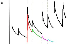
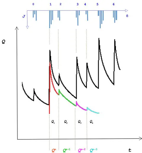
The basic procedure to reconstruct the event water response has already been demonstrated in Hoeg (2019), where the single components $Q^e$, $Q^{e-1}\dots Q^{e-\tau }$ were arranged in the following way: Assume we are interested in the event water contribution of event 1 during events 2, 3, and 4. In this case, I can arrange one after the other, in which we have the event water $Q^e$ of event 1, the last event water $Q^{e-1}$ of event 2, the second-to-last event water $Q^{e-2}$ of event 3, and the third-to-last event water $Q^{e-3}$ of event 4, as illustrated in Figure 1.

When referring to the rainfall events $J_1,J_2,\dots ,J_{\tau +1}$ and the related catchment responses $Q_1,Q_2,\dots ,Q_{\tau +1}$, I can define the separated event water response as follows:

This is the volume flow of the water that entered the catchment at interval $[t_1,t_2[$ with rainfall $J_1$, which appears in the stream discharge $Q$ during interval $[t_1,t_{1+\tau +1}[$, here as a result of the rainfall events $J_1,J_2,\dots ,J_{\tau +1}$ and the related catchment responses $Q_1,Q_2,\dots ,Q_{\tau +1}$.

Furthermore, I postulate that the volume-weighted function of the time-varying separated event water response (H_{[t_i,t_{i + 1}]} ) can be considered an approximation of the time-varying backward travel time distribution, (\stackrel{\leftarrow}{h}(\varphi, t) ), on the time interval (t \in [t_i, t_{i + \tau + 1}] ) when it comes to all water molecules that entered the catchment (the control volume of system (1)) at (t_{$\mathrm{in}$} \in [t_i, t_{i + 1}[:

, respectively

regarding the semantic time intervals $e,e+1,\dots ,e+\tau$ on $\tau$ backward iterations.

Figure 3: Alp catchment: Four years time series (June 2015-May 2019) of daily stream discharge $[\mathrm{mm}/\mathrm{d}]$ and precipitation [mm/d], temperature ${[}^{\circ }\mathrm{C}]$, and snow depth [cm], as well as ${\delta }^{18}\mathrm{O}$ composition in discharge and precipitation $[\mathrm{\%}]$ (Von Freyberg et al. (2022)). Tracer concentrations in precipitation are area weighted according to the hypersometric curve. The snow depths are retrieved from ERA5 as part of the Copernicus Climate Change Services (Hersbach et al. (2019)

III. STUDY SITE AND DATA

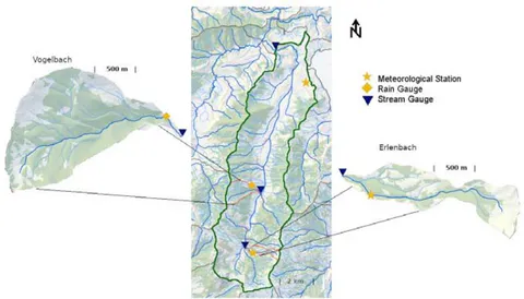
According to Von Freyberg et al. (2022) the $46.4{\mathrm{km}}^2$ Alp catchment is located near the city of Einsiedeln in central Switzerland (Figure 2). The

Figure 4: Erlenbach catchment: Four years time series (June 2015-May 2019) of daily stream discharge [mm/d] and precipitation [mm/d], temperature ${[}^{\circ }\mathrm{C}]$, and snow depth [cm], as well as ${\delta }^{18}\mathrm{O}$ composition in discharge and precipitation $[\mathrm{\%}]$ (Von Freyberg et al. (2022)). Tracer concentrations in precipitation are area weighted according to the hypso- metric curve catchment spans an elevation range of $1058\mathrm{m}$, with the outlet at $840\mathrm{m}$ above sea level and highest summit (Grosser Mythen) at $1898\mathrm{m}$ above sea level. The average slope of the Alp catchment is ${16}^{\circ }$ with a flat valley bottom and very steep slopes of up to ${75}^{\circ }$ at the south-western catchment boundary. The $0.7{\mathrm{km}}^2$ Erlenbach catchment is located on the eastern side of the Alp valley (elevation range from 1080 to $1520\mathrm{m}$ above sea level), whereas the $1.6{\mathrm{km}}^2$ Vogelbach catchment is located on the western side (elevation range from 940 to $1480\mathrm{m}$ above sea level).

The bedrock geology of the Alp catchment consists of tertiary flysch (sandstone, limestone, clays, and marls) and subalpine molasse (conglomerates, sandstone, and marls); the valley bottoms are overlain by gravel and landslide material from the adjacent hillslopes. Soils are generally shallow, with low permeability. The flanks of the Alp catchment are dominated by forests, grasslands, and wetlands, and the valley bottom is dominated by summer pastures and settlements. Van Meerveld et al. (2018) mention that the Alp tributaries are wet throughout most of the year. This is due to the high clay content, the low drainable porosity and shallow soils. The water table is generally close to the soil surface, especially in hollows and flatter areas, where the hydraulic gradient is low or at the bottom of hillslopes because of the large amount of water coming from upslope areas. Surface soil

Figure 5: Vogelbach catchment: Four years time series (June 2015-May 2019) of daily stream discharge [mm/d] and precipitation [mm/d], temperature $[\mathrm{C}]$, and snow depth [cm], as well as ${\delta }^{18}\mathrm{O}$ composition in discharge and precipitation $[\mathrm{\%}]$ (Von Freyberg et al. (2022)). Tracer concentrations in precipitation are area weighted according to the hypso- metric curve moisture measurements show that soil moisture is lowest in the forested ridge sites and highest in the flatter meadow and wetland sites.

Total annual precipitation in the Alp valley is strongly controlled by elevation, averaging $1791\mathrm{mm}$ /year in the flat northern part near the outlet, and roughly $30\mathrm{\%}$ more in the mountainous headwaters of the catchment (2300 mm/year). Snowfall comprises up to one-third of the total precipitation in the headwaters of the Alp, although snowfall is frequently interrupted by rainfall during mild periods in winter, with a corresponding occurrence of rain-on-snow events (Rucker et al. (2019)).

The ratio of current to potential evapotranspiration (ETa/ETp ratio) serves as a valuable indicator of water availability for plants. When this ratio falls below 0.8, it suggests an increased likelihood of drought-related impairments (Allgaier Leuch et al. (2017)). In the Alp catchment, we can expect ETa/ETp values to range from 0.61 to 0.9 in the valley bottoms, and from 0.81 to 1.00 in the upslope areas. These figures are based on the long-term average spanning from 1981 to 2010.

In the present study, a four-years time series (June 2015-May 2019) of daily stable water isotope data in stream water and precipitation is used for the analysis of seasonal variations. The data set is described by Von Freyberg et al. (2022), who provided detailed information on the precipitation and

Figure 6: Erlenbach catchment: High-frequency measurements of stream discharge [mm/10 minutes], and precipitation [mm/10 minutes], as well as ${\delta }^{18}\mathrm{O}$ composition in discharge and precipitation $[\mathrm{\%}]$ between September 19, 2017 and October 21, 2017 (Von Freyberg et al. (2018)) streamwater sampling, sample handling and isotope analysis. Streamwater isotopes were measured in the Alp main stream and in two of its tributaries (Erlenbach and Vogelbach). Precipitation isotopes were measured at two grassland locations in the Alp catchment: in the headwaters at $1228\mathrm{m}$ a.s.l. and near the outlet at $910\mathrm{m}$ a.s.l. The data set also includes the daily time series of key hydrologic and meteorologic variables, such as daily streamwater and precipitation fluxes, air temperature, relative humidity, and snow depth.

To better classify single rainfall runoff events and seasonal relationships, the hydrological data were supplemented with meteorological data (e.g., amount of snowfall, evapotranspiration, soil moisture) from ERA5. The reanalysis product ERA5 has recently been released by European Centre for Medium-Range Weather Forecasts (ECMWF) as part of Copernicus Climate Change Services (Hersbach et al. (2019)). This product covers the period from 1979 to present.

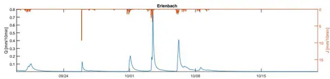
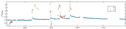
Figures 3, 4, and 5 show excerpts of the data set published via Von Freyberg et al. (2022) regarding the Alp main stream and Erlenbach and Vogelbach tributaries. In addition, Figure 6 shows an excerpt of a data set with high frequency measurements (10-minute time interval) published by Von Freyberg et al. (2018) for the Erlenbach tributary.

IV. RESULTS AND DISCUSSION

a) Estimating the Time-Varying Backward Travel Time Distribution for Single Events

The calculated event, recent, and pre-recent runoff components can be used to estimate time-varying backward travel time distributions. In the following, I demonstrate this on the basis of a simple example. Five rainfall runoff events, taken from a field study in the Erlenbach catchment between September 2016 and October 2017 (Von Freyberg et al. (2018)), serve as the examples. The analysis is based on the separation model (6) applying three backward iterations $(\tau =3)$. To determine the end member concentrations $C_Q^e,C_Q^{e-1},\dots ,C_Q^{e-3}$ and $C_Q^p,C_Q^{p-1},\dots ,C_Q^{p-3}$, differential equations (13) and (14) are not explicitly solved; instead, the pre-event water concentrations are taken directly from the measured isotope compositions in the discharge right before the hydrograph rises. The event water concentrations refer to the volume-weighted isotope composition in the respective precipitation event. For calculating the Gaussian standard errors, an uncertainty at the scale of the discharge measurements in the field, $u(Q)=0.001[{\mathrm{m}}^3/\mathrm{s}]$, and of the isotope analysis in the laboratory is adopted, that is, $u(C_Q)=0.09[\mathrm{\%}]$, $u(C_Q^e)=0.09[\mathrm{\%}]$, $u(C_Q^p)=0.09[\mathrm{\%}]$, and continuously added for each backward iteration: $u(C_Q^{e-1})=0.18[\mathrm{\%}]$, $u(C_Q^{p-1})=0.18[\mathrm{\%}]$, $u(C_Q^{e-2})=0.27[\mathrm{\%}]$, $u(C_Q^{p-2})=0.27[\mathrm{\%}]$, $u(C_Q^{e-3})=0.36[\mathrm{\%}]$, and $u(C_Q^{p-3})=0.36[\mathrm{\%}]$.

Figure 7 shows the separated event water response according to equation (22) and Figure 1 for five rainfall runoff events between September 19, 2017 and October 21, 2017. The volume-weighted version of this time-varying response can be considered an approximation of the time-varying backward travel time distribution, as shown in equation (23). In addition, the so-called rapid mobilization of pre-event water can be detected. For instance, in the magnified section of event no. 4, event water from the previous events 1-3 still occur at the catchment outlet. Von Freyberg et al. (2018) reported that pre-event water is more efficiently mobilized under wetter conditions, showing that the rapid activation of the pre-event water at Erlenbach (even during small storms) can be explained by generally shallow perched groundwater tables in the aquifer overlying the low permeability bedrock.

The median Gaussian standard error for the calculated event, recent, and pre-recent runoff components are $u(Q^e)=81.9\mathrm{\%}/0.01\frac{\mathrm{mm}}{10\min }$, $u(Q^{e-1})=123.4\mathrm{\%}/0.10\frac{\mathrm{mm}}{10\min }$, $u(Q^{e-2})=205.2\mathrm{\%}/0.18\frac{\mathrm{mm}}{10\min }$, $u(Q^{e-3})=231.6\mathrm{\%}/0.07\frac{\mathrm{mm}}{10\min }$, and $u(Q^{p-3})=32.3\mathrm{\%}/0.18\frac{\mathrm{mm}}{10\min }$. For better illustration, Figure 8 shows the separated event water response for a single rainfall runoff event (number 3) together with the Gaussian standard error bounds according to equation (15).

Figure 9: Monthly Pardé coefficients (1: January - 12: December) of stream discharge Q, event water $Q^e$, recent water $Q^{r-3}$, pre-recent water $Q^{p-3}$, precipitation (J), and evapotranspiration (ET) for the Erlenbach, Vogelbach, and Alp catchments, based on the four-year investigation between June 2015 and May 2019, and an iterative extension of the standard two-component hydrograph separation method. Evapotranspiration data are taken from the reanalysis product ERA5

b) Seasonal Variations of Event, Recent and

In the following, an analysis of the runoff generation processes in terms of event $Q^e$, recent $Q^{r-3}$, and pre-recent $Q^{p-3}$ runoff components is demonstrated for the pre-Alpine Alp catchment (46.4 km2) and two smaller tributaries (Erlenbach, 0.7 km2, and Vogelbach, 1.6 km2), whereas recent water is understood as the contribution of the respective three prior rainfall-runoff events, that is

To compensate for altitude effects on the catchment scale, the daily isotope concentrations in precipitation considers the available isotopic samples of the two measuring stations and are area weighted based on to the hypsometric curve of the Alp catchment. The analysis is based on the separation model (6) that applies three backward iterations $(\tau =3)$, whereas the entire data set is being processed; that is, 147 rainfall runoff events are being investigated for the Alp catchment, 113 rainfall runoff events for the Erlenbach catchment, and 120 rainfall runoff events for the Vogelbach catchment. Again, the end member concentrations $C_Q^e,C_Q^{e-1},\dots ,C_Q^{e-3}$ and $C_Q^p,C_Q^{p-1},\dots ,C_Q^{p-3}$ are taken directly from the concentrations in the stream

Figure 10: Monthly Pardé coefficients (1: January - 12: December) of event water $Q^{\mathrm{e}}$, recent water $Q^{\mathrm{r}-3}$, and pre-recent water $Q^{\mathrm{p}-3}$ for the Erlenbach, Vogelbach, and Alp catchments in relation to the monthly Pardé coefficients of stream discharge (Q) in%, based on the four-year investigation between June 2015 and May 2019, and an iterative extension of the standard two-component hydrograph separation method discharge and precipitation. In addition, where necessary, the end member concentrations are partially adjusted to ensure that Criterion 4 (equation (7)) is continuously fulfilled. This approach does not reduce or increase the size of the relative error, but it does stabilize the solution overall (Hoeg (2021)). Although the absolute Gaussian standard error bounds are moderately low with values between $0.09\mathrm{mm}/\mathrm{d}$ and $0.61\mathrm{mm}/\mathrm{d}$ (see Table 1), the relative errors associated with this hydrograph separation are relatively high, with values between $38.5\mathrm{\%}$ and $622.4\mathrm{\%}$. Therefore, the results may not lead to accurate quantitative conclusions. Nevertheless, qualitative statements about the seasonal runoff formation in the Alpine catchment area and its tributaries Erlenbach and Vogelbach are possible, as I will show below.

To visualize the seasonal variations, I calculate the Pardé coefficients for each runoff component, which is the quotient of the long-term (four years) average monthly discharge and long-term (four years) average annual discharge. The precipitation and evapotranspiration regimes are added to better evaluate and classify the monthly and seasonal changes of the runoff components, which are: stream discharge $Q$, event water $Q^e$, recent water $Q^{r-3}$, and pre-recent water $Q^{p-3}$. Evapotranspiration data are taken from the reanalysis product ERA5 of the Copernicus Climate Change Service. For the Alp catchment and its tributaries, a nivale runoff and precipitation regime can

Figure 11: Added monthly Pardé coefficients (1: January - 12: December) of event water $Q^{\mathrm{e}}$, recent water $Q^{\mathrm{r}-3}=Q^{\mathrm{e}-1}+Q^{\mathrm{e}-2}+Q^{\mathrm{e}-3}$, and pre-recent water $Q^{\mathrm{p}-3}$ for the Erlenbach, Vogelbach, and Alp catchments in relation to the monthly Pardé coefficients of stream discharge (Q). Monthly Pardé coefficients (1: January - 12: December) of precipitation (J), and evapotranspiration (ET), based on the four-year investigation between June 2015 and May 2019, and an iterative extension of the standard two-component hydrograph separation method. Evapotranspiration data are taken from the reanalysis product ERA5 be shown in Figure 9. In relation to the stream discharge Q, the event water component $Q^e$ has its maximum during August in general, as shown in Figure 10 and Figure 11. The highest recent water fractions $Q^{r-3}$$(50-59\mathrm{\%})$ can be expected at the beginning of winter (December, January), whereas the lowest fractions $(7-14\mathrm{\%})$ are found at the end of autumn (November). In return, higher pre-recent water fractions $Q^{p-3}$ can be found in the summer (July, $60-82\mathrm{\%}$ ) and in the middle of autumn (October, $64-74\mathrm{\%}$ ). The two tributaries expose an additional peak of pre-recent water in the snowmelt season (April, $47-62\mathrm{\%}$ ), during which the lowest event water fractions $(6-8\mathrm{\%})$ can be expected. For the Alp catchment, the event water component $(29-32\mathrm{\%})$ and recent water component $(56\mathrm{\%})$ clearly exceed the pre-recent component $(17-21\mathrm{\%})$ in August and September after the month July, which is characterized by relatively low precipitation, high evapotranspiration, and low soil moisture.

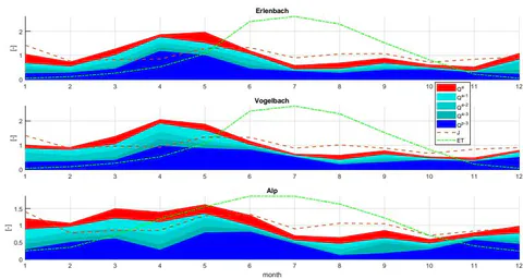
A sensitivity analysis regarding the evapotranspiration rates ET from ERA5 confirms the calculated seasonal variations of the Pardé coefficients both for the Alp catchment and its tributaries, Erlenbach and Vogelbach. The analysis, shown in Figure 12, indicates a shift in proportions towards

Figure 12: Added monthly $Pardé$ coefficients (1: January - 12: December) of event water $Q^e$, recent water $Q^{r-3}=Q^{e-1}+Q^{e-2}+Q^{e-3}$, and pre-recent water $Q^{p-3}$ for the Erlenbach, Vogelbach, and Alp catchments in relation to the monthly $Pardé$ coefficients of stream discharge (Q). Monthly $Pardé$ coefficients (1: January - 12: December) of precipitation (J), and evapotranspiration (ET), based on the four-year investigation between June 2015 and May 2019, and an iterative extension of the standard two-component hydrograph separation method. Sensitivity analysis to assess the impact of ET on the daily end member concentrations $(C_Q^e,C_Q^{e-1},\dots ,C_Q^{e-3})$. This analysis involves considering a rate factor $f_{ET}$, which can take values of 0.25 or 0.5. To first-order approximate the daily end member concentrations, the daily precipitation rates (J) are directly reduced by $25\mathrm{\%}$ or $50\mathrm{\%}$ of the daily evapotranspiration rates, similar to equation (13). The evapotranspiration data used in this analysis are obtained from the reanalysis product ERA5.

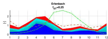
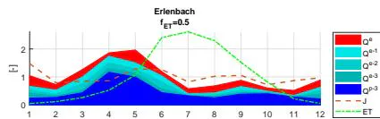
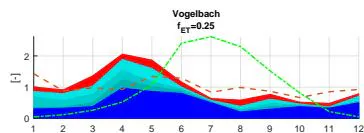
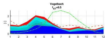
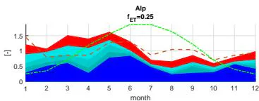
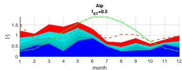
the event water component (up to $5\mathrm{\%}$ in August) and pre-recent water component (up to $20\mathrm{\%}$ in August) when daily evapotranspiration rates are considered up to $50\mathrm{\%}$ when calculating daily end member concentrations $C_Q^e,C_Q^{e-1},\dots ,C_Q^{e-3}$. However, for the Alp catchment, the event water component and recent water component still exceed the pre-recent component in August and September.

The latter result is noteworthy because, on the one hand, it confirms that considerable fractions of summer precipitation become streamflow, even though evapotranspiration fluxes are much larger in the summer (Allen et al. (2019)); on the other hand, it shows that a certain limit appears to have been reached in the Alp catchment for the months of August and September. A further increase of hydrological drought in central Europe (Balting et al. (2021), Satoh et al. (2022)) is unlikely to lead to a greater mobilization and availability of pre-recent runoff components in this area. Consequently, the

Component	Erlenbach	Vogelbach	Alp
QE	84.1/0.09	622.4/0.09	144.4/0.12
QR-3	161.6/0.50	142.9/0.49	159.1/0.93
QP-3	50.0/0.26	38.5 /0.28	74.3/0.61

importance of event water and recent water for the catchment water balance will continue to increase, and with lower rainfall and/or higher temperatures in the summer months, the situation for vegetation, which relies on the remaining summer precipitation, might become even worse than observed in the past few years and decades, as noted by Senf et al. (2018), and Senf et al. (2020). If climate projections prove to be accurate, there will be a significant increase in drought conditions across extensive areas of the Swiss forest by the conclusion of the 21st century. Nevertheless, the duration of drought will increase the most by the year 2100 in those forest site types that are already relatively dry today. The least vulnerable are forest sites in areas with very high precipitation and cool temperatures, on deep or hydromorphic soils. (Scherler et al. (2016)).

V. CONCLUSIONS

In the present study, I have shown that the classic two-component hydrograph separation can be iteratively embedded in a discretization of the catchment water and tracer mass balance along the event and pre-event time axis. With this method, it is possible, for instance, to analyze and quantify the rapid mobilization of recent water for single (high-frequency measured) rainfall-runoff events, and to estimate time-varying backward travel time distributions. When applied to longer time series of daily stable water isotope data in stream water and precipitation, the method can be used to analyze seasonal variations of event, recent, and pre-recent runoff components.

In relation to the Alp catchment, the relatively high fractions of event water and recent water in stream discharge during August and September represents a rather unexpected result that certainly requires further investigation, but shows that fundamental assumptions, used for instance in runoff recession analysis, need to be questioned and that the sensitivity of the catchment water balance in response to drought situations could be greater than expected.

Moving forward, there are opportunities to further refine the method, apply it to new contexts, or integrate it with other techniques. For example, the method can be used to examine the event, recent, and pre-recent components in the evapotranspiration (volume flow $ET$ ) or in the ground-water recharge (volume flow $\mathrm{d}S/\mathrm{d}t$ ) of a catchment. In addition, there is the potential to incorporate this approach into hydrological models to improve their accuracy and predictive capabilities. Moreover, there are opportunities to apply the method in more complex and detailed ways, potentially uncovering new insights in catchment hydrology. This could include, for instance, more detailed analyses of the impacts of extreme weather events or the effects of different land use practices.

ACKNOWLEDGEMENTS

The author would like to thank Jana von Freyberg (ETH - Swiss Federal Institute of Technology Zurich, Department of Environmental Systems Science) for providing the additional excerpt of the high-frequency measurement series from the Erlenbach catchment. My special thanks goes to chief editor Marie V. Carlsen, assistant editor Marian C. Miller, and two anonymous reviewers, who contributed to this work with numerous improvement proposals.

Data and Code Availability

The data used for this study can be retrieved via Von Freyberg et al. (2018) and Von Freyberg et al. (2022). Complementary data from ERA5 (fifth generation of ECMWF reanalysis for the global climate and weather) are available at https://cds.climate.copernicus.eu/. The Matlab scripts, together with some supplementary material, will be available at https://osf.io/azrqw/.

Appendix A. Notation

Appendix A.1. Latin Symbols

{"algorithm_caption":[],"algorithm_content":[{"type":"equation_inline","content":"C_{$\dot{V}$}"},{"type":"text","content":" tracer concentration in volumetric flow \n "},{"type":"equation_inline","content":"C_{$\dot{V}$}^{e}"},{"type":"text","content":" tracer concentration event water in volumetric flow \n "},{"type":"equation_inline","content":"C_{$\dot{V}$}^{p}"},{"type":"text","content":" tracer concentration pre-event water in volumetric flow \n "},{"type":"equation_inline","content":"ET"},{"type":"text","content":" evapotranspiration \n "},{"type":"equation_inline","content":"h"},{"type":"text","content":" travel time distribution, impulse response function \n "},{"type":"equation_inline","content":"\overleftarrow{h}"},{"type":"text","content":" backward travel time distribution \n "},{"type":"equation_inline","content":"\overrightarrow{h}"},{"type":"text","content":" forward travel time distribution \n "},{"type":"equation_inline","content":"$\hat{h}$"},{"type":"text","content":" residence time distribution \n "},{"type":"equation_inline","content":"H"},{"type":"text","content":" separated event water response \n "},{"type":"equation_inline","content":"J"},{"type":"text","content":" precipitation \n "},{"type":"equation_inline","content":"Q"},{"type":"text","content":" stream discharge \n "},{"type":"equation_inline","content":"Q^{e}"},{"type":"text","content":" event water in stream discharge \n "},{"type":"equation_inline","content":"Q^{p}"},{"type":"text","content":" pre-event water in stream discharge \n "},{"type":"equation_inline","content":"Q^{r}"},{"type":"text","content":" recent water in stream discharge \n "},{"type":"equation_inline","content":"S"},{"type":"text","content":" water storage \n "},{"type":"equation_inline","content":"t"},{"type":"text","content":" time \n "},{"type":"equation_inline","content":"t_{$\mathrm{in}$}"},{"type":"text","content":" injection time \n "},{"type":"equation_inline","content":"V"},{"type":"text","content":" volumetric flow rate \n "},{"type":"equation_inline","content":"${\dot{V}}^e$"},{"type":"text","content":" event water in volumetric flow \n "},{"type":"equation_inline","content":"${\dot{V}}^p$"},{"type":"text","content":" pre-event water in volumetric flow "}]}

Appendix A.2. Greek Symbols

θ	partition function
τ	backward iteration
φ	travel time
ω	age function

Appendix B. Linear Equation System for Three Backward Iterations

The iterative separation model (6) can be represented in the form of a linear equation system for $\tau =3$, as follows:

[1 1 0 0 0 0 0 0]	[1 1 0 0 0 0 0 0]	[1 1 0 0 0 0 0 0]
CeV CpeV 0 -1 1 1 0 0 0 0	CpeV CpeV 0 -1 1 1 0 0 0 0]	CpeV CpeV 0 -1 1 1 0 0 0]
0 -1 0 0 -1 1 1 0 0 0]	0 -1 1 1 0 0 0 0]	0 -1 1 1 0 0 0]
0 -1 0 0 -1 1 1 0 0 0]	0 -1 1 1 0 0 0 0]	0 -1 1 1 0 0 0]
0 -1 0 0 -1 1 1 0 0 0]	0 -1 1 0 0 0 0]	0 -1 1 0 0 0]