Lehmann Type-2 Inverse Lomax Distribution and Applications to Reliability Data

Olayode Fatoki; Adeleye Najeem Friday; Adefolarin David Adekunle

I. INTRODUCTION

Over the last century, many significant distributions have been introduced to serve as models in applied sciences. The notable among them, generalized beta distribution developed by McDonald (1995), is at the top of the list in terms of usefulness. The main feature of the generalized beta distribution is that it introduces skewness and kurtosis into the baseline distribution that allows for modeling data of various forms of the shape of the hazard function which may be decreasing, increasing, decreasing-increasing, increasing decreasing, and inverted bathtub shapes. In this paper, we focus our attention on one of the most attractive of these distributions, known as the inverse Lomax $(IL)$ distribution. Mathematically, it can be presented in the distribution form as $\mathrm{Y} = X^{-1}$ , where $\mathbf{X}$ is a random variable following the famous Lomax distribution (see Lomax, 1954). Thus, the cumulative distribution function (CDF) of the $IL$ distribution is given by

where $\pmb{\rho}$ is a positive scale parameter and $\lambda$ is a positive shape parameter. The reasons for studying the IL distribution are not limited to the following: It has proved itself as a statistical model in various applications, including economics and actuarial sciences (see Kleiber and Kotz, (2003)) and geophysics (see McKenzie et al. (2004)). Also, the mathematical and inferential aspects of the IL distribution have been studied. See, for example, Lorenz (2004), for the Lorenz ordering of order statistics, Rahman and Aslam

(2013) studied the estimation of the parameters in a Bayesian setting, Yadav et al. (2016) examined the estimation of the parameters from hybrid censored samples, Singh et al. (2016) the study of the reliability estimator under type II censoring and Reyad, and Othman (2018) studied the Bayesian estimation of a two-component mixture of the IL distribution type I censoring. Despite an interesting compromise between simplicity and accuracy, the IL model suffers from a certain rigidity in the peak (punctual and roundness) and tail properties. This motivates the development of various parametric extensions, such as the inverse power Lomax distribution introduced by Hassan and Abd-Allah 92018), the Weibull IL distribution studied by Hassan, A.S.; Mohamed (2019) and, the Marshall-Olkin IL distribution developed by Maxwell et al. (2019). In this paper, we introduce and discuss a new extension of the IL distribution called Lehman Type-2 Inverse Lomax distribution which can model all forms of data exhibiting any shape of the hazard function because of its flexibility and tractability.

II. LEHMANN TYPE-2 INVERSE LOMAX DISTRIBUTION

The CDF of the Lehmann type-2 family of distribution is given by

And the associated PDF is given by

Putting (3) and (4) in (2), we have an expression for the Lehmann Type-2 inverse Lomax (LT-2IL) distribution given by

The survival and the hazard function are respectively given by

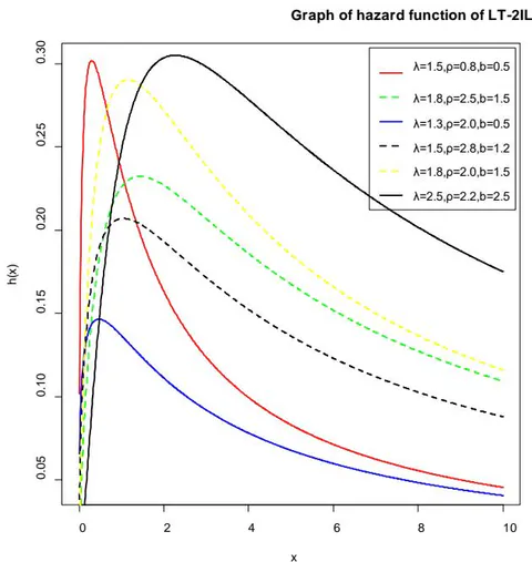
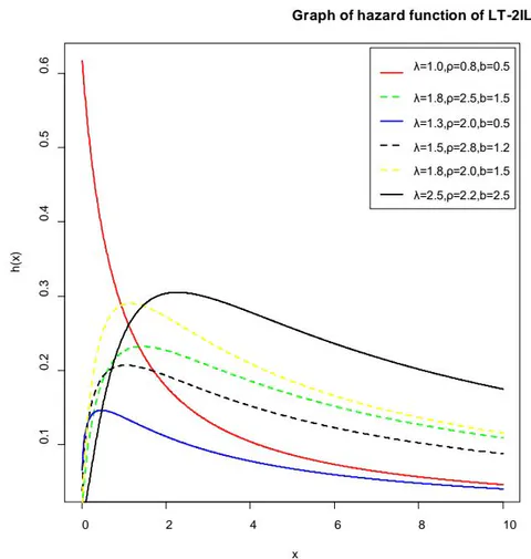
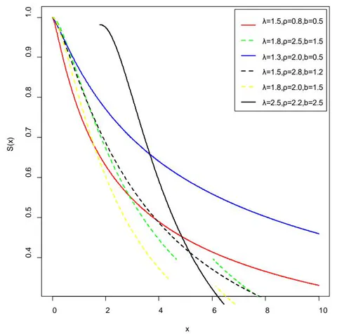
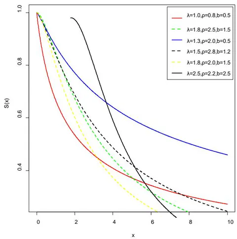
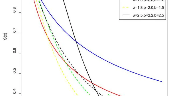
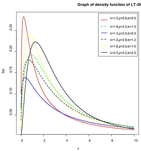
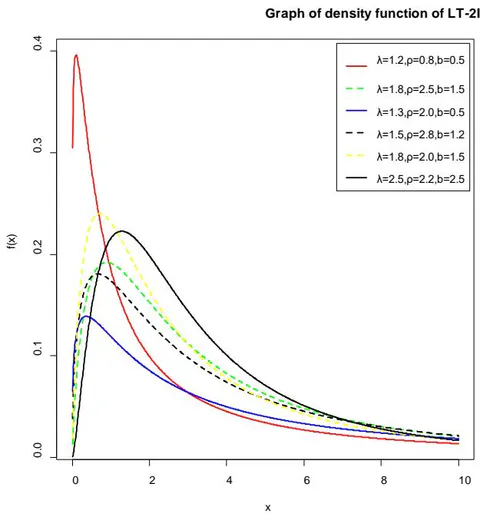
The graph of the density, hazard, and the survival function is given in figures 1, 2, and 3 for various values of the parameters.

Notes

Figure 1: The graph of the density function of LT-2IL distribution

Figure 2: The graph of the hazard function of LT-2IL distribution

Graph of survival function of LT-2IL

Graph of survival function of LT-2IL Figure 3: The graph of the survival function of

LT - 2IL

distribution

III. USEFUL EXPANSIONS

The binomial theorem, for $m > 0$ and $|v| < 1$ , can be expressed as follows: $(1 - v)^{m} = \sum_{i=0}^{\infty} (-1)^{i} \binom{m}{i} v^{i} \tag{9}$

Then, applying the binomial series expansion given in (9) to (5), we have

Finally, we have

Equation (10) represents the Exponentiated Inverse Lomax distribution, with shape parameter $[\lambda (i + 1) + 1]$ and scale parameter $\rho$ . It then follows that the properties of Lehmann type-2 inverse Lomax distribution can be obtained from that of the Exponentiated inverse Lomax distribution.

a) Quantile function

The quantile function of the $LT - 2IL$ distribution is defined by $Q(u; b, \lambda, \rho) = F^{-1}(u; b, \lambda, \rho)$ , $u \in (0,1)$ . After some mathematical manipulations, we obtain

From (10.1), we can obtain the lower quartile $(q_{1})$ , middle quartile $(q_{2})$ , also known as the median, and the upper quartiles $(q_{3})$ of the $LT - 2IL$ distribution by taking the values of $u$ to be 0.25, 0.5, and 0.75 respectively. Then, we obtain an equation for the lower quartile, median, and the upper quartile of $LT - 2IL$ distribution given respectively, by

and

b) Moments of LT - 2IL distribution

The $k^{th}$ moment of the $LT - 2IL$ distribution under certain regularity conditions; the $k^{th}$ moment of TIIHLF distribution is obtained as

where

Taking $z = \frac{\rho}{x}$ and putting it in (12), we have

Also, letting $y = \frac{v}{1 - v}$ , $dy = (1 - v)^{-2} dv$ and putting it in (13), we have

Finally, we obtain an expression for the $k^{th}$ moment of the $LT - 2IL$ distribution given as

Where $B(.,.)$ is a beta function

An expression for the first, second and third moments can be obtained by respectively taking the value of $k = 1,2$ and 3 as

And

c) Incomplete moments of LT-2IL distribution

The incomplete moment of LT-2IL distribution can be obtained using (13) as

where

Taking $z = \frac{\rho}{x}$ and putting it in (17), we have

Also, letting $y = \frac{v}{1 - v}$ , $dy = (1 - v)^{-2} dv$ and putting it in (18), we have

Then we have

Finally, we obtain an expression for the $k^{th}$ incomplete moment of the $LT - 2IL$ distribution given as

d) Renyi entropy

Renyi entropy was proposed by Renyi (1961). It can be obtained by

Where

Putting (5) in (28) followed by binomial expansion, we have

Taking $y = \frac{\rho}{x}$ , $dx = -\rho y^{-2} dy$ , putting it in (30), we have

Furthermore, by letting $y = \frac{u}{1 - u}$ , $dw = (1 - u)^{-2}du$ and putting it in (31) gives

Finally, we have an expression for the Renyi entropy of LT-2IL distribution as

e) Tsallis Entropy

The Tsallis entropy, also known as $\beta$ -entropy, was first discovered by Havrada and Charvat (1967) and later developed by Tsallis (1988). The Tsallis entropy of the LT-2IL distribution can be defined as

Invariably, it may be written as

Putting (29) in (32), we obtain an expression for the Tsallis entropy given as

f) Order statistics

Let $X$ be a random variable from the KGIL distribution and, given a random sample size $n$ from $X$ , say say $X_{1},\ldots,X_{n}$ , let $x_{i:n}$ be the $i^{th}$ order statistic such that $x_{1:n}\leq x_{2:n}\leq x_{3:n}\leq \dots \leq x_{n:n}$ , given that $x_{h:n}\in \{X_1,\ldots,X_n\}$ for $h = 1,\ldots,n$ . In particular, the study of order statistics is very important since naturally it appears in many applications, majorly those involving systems comprises of several components parts that can fail independently of each other. The density of $x_{i:n}$ is given by

Applying binomial theorem given in (36) to the expression above, it follows immediately that

Putting (5) and (7) in (37) gives us the following series expansion for the $i^{th}$ order statistics for $LT - 2IL$ distribution as

It should be noted that from (38) an expression for the smallest and the largest order statistics can be obtained.

IV. MAXIMUM LIKELIHOOD ESTIMATION (MLE) METHOD

Taking an observed sample $x_{1},\ldots,x_{n}$ from the $LT - 2IL$ distribution, the corresponding likelihood function can be represented as

The MLEs of $p, q, \beta$ , and $\lambda$ are denoted by $\hat{b}, \hat{\pmb{p}}$ , and $\hat{\lambda}$ , respectively. The log-likelihood function is given by

And the element of the score vector is given by

V. APPLICATIONS

In this section, two life-time data sets are provided to illustrate the importance of the $LT - 2IL$ distribution in modeling life-time data. We compare the $LT - 2IL$ model with other competitive models such as Kumaraswamy inverse Lomax (KIL), Kumaraswamy Frechet (KF), Exponentiated Lomax (EL), and the inverse Lomax (IL) distribution.

To check the adequacy of the fitted model in fitting the data considered, Akaike information criterion (AIC), consistent Akaike information criterion (CAIC), Bayesian information criterion (BIC), Kolmogorov-Smirnov(KS), Crammer-Von Misses (CM), Anderson Darling(AD) goodness of fit test and its p-value (PV) are obtained. In general, it is considered that the smaller the values of AIC, BIC, CAIC, HQIC and, K statistics and the larger the p-value, the better the fit of the model.

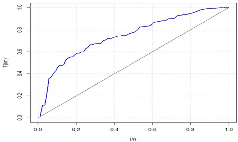
Figure 4: Graph of the total time on test plot for Jet air conditioning data

Table 5739: Table 1: MLEs and standard errors in braces for the first data set

Model	λ	ρ	b	a
LT-2IL	1.247(0.199)	125.111(77.185)	2.7769(0.961)	-(-)
EL	0.6547(0.161)	1.2489(0.368)	15.558(4.407)	-(-)
KIL	0.7724(18.669)	144.4729(101.187)	1.565(37.835)	3.0006(1.204)
KF	0.6137(0.110)	0.6451(0.1625)	8.8399(1.675)	5.001(1.353)
IL	2.0790(0.395)	18.822(4.938)	-(-)	-(-)

Table 5738: Table 2: AIC, BIC, CAIC, CM, AD KS statistic, and P- value (PV) for first data set

Model	-1	AIC	BIC	CAIC	CM	AD	KS	PV
LT - 2IL	1034.77	2075.54	2085.25	2075.68	0.057	0.415	0.050	0.736
EL	1054.88	2115.77	2125.48	2115.90	0.357	2.393	0.089	0.099
KIL	1034.74	2077.69	2090.42	2077.69	0.061	0.433	0.049	0.741
KF	1039.52	2087.03	2099.98	2087.25	0.115	0.842	0.052	0.687
IL	1044.10	2092.20	2098.67	2092.26	0.173	1.175	0.068	0.343

The second data sets have been obtained from Murthy et al. (2004) is about the failure times of windshields and is given by 0.04, 0.3, 0.31, 0.557, 0.943, 1.07, 1.124, 1.248, 1.281, 1.281, 1.303, 1.432, 1.48, 1.51, 1.51, 1.568, 1.615, 1.619, 1.652, 1.652, 1.757, 1.795, 1.866, 1.876, 1.899, 1.911, 1.912, 1.9141, 0.981, 2.010, 2.038, 2.085, 2.089, 2.097, 2.135, 2.154, 2.190, 2.194, 2.223, 2.224, 2.23, 2.3, 2.324, 2.349, 2.385, 2.481, 2.610, 2.625, 2.632, 2.646, 2.661, 2.688, 2.823, 2.89, 2.9, 2.934, 2.962, 2.964, 3, 3.1, 3.114, 3.117, 3.166, 3.344, 3.376, 3.385, 3.443, 3.467, 3.478, 3.578, 3.595, 3.699, 3.779, 3.924, 4.035, 4.121, 4.167, 4.240, 4.255, 4.278, 4.305, 4.376, 4.449, 4.485, 4.570, 4.602, 4.663, 4.694. Some descriptive statistics for these data shows that the smallest and the largest values are 0.04 and 4.694, respectively. Further, the mean, median and variance are 2.569, 2.367 and 1.286, respectively. The Total time on test plot for the windshield data set is given in figure 4. The parameter estimates and the values for the goodness of fit test for the model is given in Table 3 and 4 respectively.

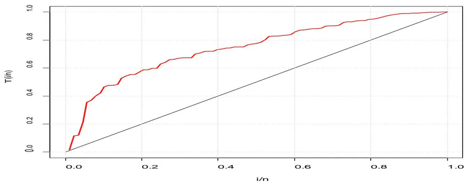
Figure 5: Graph of the total time on test plot for the second data

Table 5737: Table 3: MLEs and standard errors in braces for the second data set

Model	λ	ρ	b	a
LT-2IL	2.591(0.319)	16.442(8.468)	142.560(111.761)	-(-)
EL	1.584(0.351)	1.1683(0.348)	3.428(1.143)	-(-)
KIL	1.549(0.939)	4.3495(1.485)	1.939(1.176)	16.1458(5.434)
KF	0.7820(0.305)	1.0205(0.588)	7.163(3.946)	13.3993(8.685)
IL	4.123(1.321)	0.490(0.184)	-(-)	-(-)

Table 5736: Table 4: AIC, BIC, CAIC, CM, AD, KS statistic and P- value (PV) for the second data set

Model	-1	AIC	BIC	CAIC	CM	AD	KS	PV
LT - 2IL		283.93	291.07	283.94	0.064	0.668	0.057	0.929
EL	166.92	339.84	347.27	340.13	0.705	4.571	0.169	0.013
KIL	143.95	295.89	305.80	296.38	0.137	1.203	0.094	0.408
KF	150.68	309.83	319.26	309.83	0.272	2.078	0.121	0.152
IL	187.02	378.05	383.0	378.19	0.825	5.233	0.336	4.6e - 09

It could be observed from the results obtained from the two data sets considered that the Lehmann Type-2 Inverse Lomax model possesses the smallest AIC, BIC, CAIC, CM, AD, KS statistic and, the largest of a P-value. It could therefore be regarded as the best model in the class of the models considered based on the data used.

VI. CONCLUDING REMARKS

In this paper, we developed a study a novel three-parameter distribution called Lehmann-type-2 Inverse distribution. Some statistical properties of the new distribution are studied. The maximum likelihood estimation method is used to obtain the parameters. Two real data sets are presented to illustrate the applicability of the new model.

References

16 Cites in Article
1. Gauss Cordeiro,Artur Lemonte (2011). The <mml:math xmlns:mml="http://www.w3.org/1998/Math/MathML" altimg="si38.gif" display="inline" overflow="scroll"><mml:mi>β</mml:mi></mml:math>-Birnbaum–Saunders distribution: An improved distribution for fatigue life modeling.
2. James Mcdonald,Yexiao Xu (1995). A generalization of the beta distribution with applications.
3. K Lomax (1954). Business Failures: Another Example of the Analysis of Failure Data.
4. Christian Kleiber,Samuel Kotz (2003). Statistical Size Distributions in Economics and Actuarial Sciences.
5. D Mckenzie,C Miller,D Falk (2011). The Landscape Ecology of Fire.
6. C Kleiber (2004). Lorenz ordering of order statistics from log-logistic and related distributions.
7. Shujiao Huang,Broderick Oluyede (2014). Exponentiated Kumaraswamy-Dagum distribution with applications to income and lifetime data.
8. Jafer Rahman,Muhammad Aslam (2013). On estimation of two-component mixture inverse Lomax model via Bayesian approach.
9. A Yadav,S Singh,U Singh (2016). On hybrid censored inverse Lomax distribution: Application to the survival data.
10. Sanjay Singh,Umesh Singh,Abhimanyu Yadav (2016). Bayesian estimation of Lomax distribution under type-II hybrid censored data using Lindley's approximation method.
11. H Reyad,S Othman (2018). E-Bayesian estimation of two-component mixture of inverse Lomax distribution based on type-I censoring scheme.
12. Amal Hassan,Marwa Abd-Allah (2018). On the Inverse Power Lomax Distribution.
13. A Hassan,R Mohamed (2019). Weibull inverse Lomax distribution.
14. Obubu Maxwell,Angela Chukwu,Oluwafemi Oyamakin,Mundher Khaleel (2019). The Marshall-olkin Inverse Lomax Distribution (MO-ILD) with Application on Cancer Stem Cell.
15. D Murthy,M Xie,R Jiang (2004). Weibull Models.
16. Constantino Tsallis (1988). Possible generalization of Boltzmann-Gibbs statistics.
Funding
No external funding was declared for this work.
Conflict of Interest
The authors declare no conflict of interest.
Ethical Approval
No ethics committee approval was required for this article type.
Data Availability
Not applicable for this article.
How to Cite This Article
Olayode Fatoki, Adeleye Friday, Adefolarin Adekunle. 2026. "Lehmann Type-2 Inverse Lomax Distribution and Applications to Reliability Data". Global Journal of Science Frontier Research - F: Mathematics & Decision GJSFR-F Volume 22 (GJSFR Volume 22 Issue F3).
Download Citation
Enhanced Lomax Distribution in Research.
Journal Specifications
Crossref Journal DOI 10.17406/GJSFR
Print ISSN 0975-5896
e-ISSN 2249-4626
Keywords
Classification
GJSFR-F Classification DDC Code: 536.73 LCC Code: QC318.E57
Version of record
v1.2
Issue date
September 20, 2022
Language
English
Experiance in AR
Explore published articles in an immersive Augmented Reality environment. Our platform converts research papers into interactive 3D books, allowing readers to view and interact with content using AR and VR compatible devices.
Read in 3D
Your published article is automatically converted into a realistic 3D book. Flip through pages and read research papers in a more engaging and interactive format.
Article Matrices
Total Views: 389
Total Downloads: 23
All Trends
Request Access
Please fill out the form below to request access to this research paper. Your request will be reviewed by the editorial or author team.
X
This is the heading
Lorem ipsum dolor sit amet, consectetur adipiscing elit. Ut elit tellus, luctus nec ullamcorper mattis, pulvinar dapibus leo.
High-quality academic research articles on global topics and journals.