## I. INTRODUCTION ### a) Paper Size, Margins, Columns and Paragraphs For environmental impact studies, it is vital to know the dynamics of conservative solutes moving in a flow, which simulate quite well the behavior of the pollutants poured in, and are therefore important for their understanding, control and mitigation. [1] In this perspective, the calculation of the transport coefficients, especially the one that defines the transverse diffusion, is fundamental. J. W. Elder in his original work [2], based on theoretical considerations, found a definition of the transverse diffusion coefficient, $\varepsilon y$, which have the following definition, with H as depth, g, as acceleration of gravity and S, as slope of the energy line: $$ \varepsilon y \approx 0.23 * H * \sqrt{H * g * S} \tag{1} $$ But later, H.B. Fischer [3], who varied this coefficient by about $50\%$, found better accommodation with the experimental results. This formula is used in this Article as a reference for comparing results due to its simplicity and relative accuracy. 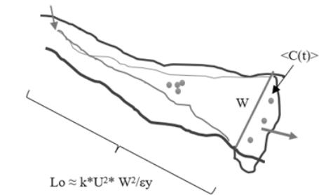This transverse diffusion coefficient plays a very important role in understanding and defining the so-called "Mixing length", Lo, the distance at which the solute transported in a flow is considered to be "mean value" distributed in the cross section, and its concentration is a relative minimum, indicating well what the "assimilation capacity of the channel" is reached. With "k" a coefficient that depends on the way the solute is injected into the flow (k=1 for central injection), U the average velocity, and W the average width [4,5]. $$ Lo \approx \frac{k*U*W^{2}}{\varepsilon y} \tag{2} $$ This equation refers to the channel's "width" and is defined when the solute diffuses at an "average" value. Although the physical basis of this equation is sufficiently proven, the fact that it is affected by the "k" factor, which varies between 0.1 and 0.4 and depends on how well the injection point is located, adds an unavoidable component of imprecision. For this reason, it is interesting to explore an alternative procedure, based on other principles, that provides greater certainty in this critical measurement. This new procedure may be based on when the solute evenly covers the cross-section of its stream tube with a homogeneous distribution, which may or may not coincide with the channel's width. Figure 1 compares the two procedures: the classic one, corresponding to equation (2), and the new approach.  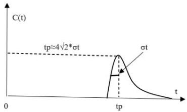This new situation occurs when the solute transport distance is long enough for almost all of its mass (99.7%) has lost most of its interactions, and its particles are distributed homogeneously like an ideal gas (losing significantly its interactions), [6] such that, according to Gauss's Theory, there is a corresponding distance of "Six sigma", when $t \approx 4\sqrt{2} \sigma t$, which if $U \approx \sigma_{x} / \sigma_{t}$, it holds. [7]: $$ L o ^ {\prime} \approx 4 \sqrt {2} * \sigma_ {x} \tag {3} $$ Defining transverse diffusion has not been easy, as there is no identifiable velocity distribution along this axis that would allow theoretical manipulation to establish mixing along this axis, as is the case on the vertical axis. [8] In water quality studies, this "complete mixing" condition is of primary importance, given that monitoring of the variables of interest, they must have optimal representativeness, ensuring that the models run appropriately.[9] This information is typically collected in the field with tracer tests. On the other hand, it is necessary to distinguish diffusion from dispersion [10]. The former is associated with transport caused by turbulence as a mixing agent, and on a much smaller scale by molecular motion. The second is more directly associated with the mixing and expansion effect of a solute due to the shear effect of longitudinal velocities, arising from the mean advective velocity. The characteristic is that both types of motion are defined as proportional to the concentration gradient.[11] Thus, while dispersion expands without limit along the longitudinal axis, transverse diffusion has a rather small limit (restricted by a finite width). Figure 2.  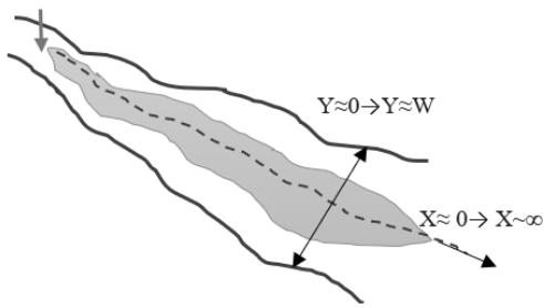Source: Author Figure 2: Different Spatial Nature of Longitudinal and Transverse Dispersion-Diffusion This implies that, due to this restriction, diffusion generally progresses much less rapidly than dispersion and can reach a certain equilibrium before its longitudinal portion, covering the cross-sectional area of the flow. Then, the application of two "complete mixing" criteria must be distinguished: One: When Lo is applicable, the channel width and the transverse diffusion coefficient must be considered primarily. and Two: When Lo' is applicable, the spatial variance of the solute curve must be considered primarily. Both criteria show important aspects of the tracer advance mechanism. The first criterion is appropriate for channels of not very great width, in which the value of "Lo" is practical for measurement. The second criterion is applied in very large rivers in which the solute behavior is well described by "Lo", without needing to refer it to the channel width. ## II. STATE FUNCTION TO DESCRIBE THE EVOLUTION OF SOLUTES IN TURBULENT FLOWS ### a) Definition of the Function and its Relationship with the Average Flow Velocity A transport model has been presented based not on the concept of "Dead zones" as the cause of the "non-Fickian bias" of the experimental tracer curves, but rather on the concept of heat exchange in the phenomena of "hydration" and "dilution", supported by the enthalpy of formation of the solute. [12] This evolution is described by a State Function $\Phi(t)$, fulfilling the Pfaff conditions [13] that has been applied to explain numerous experimental cases [14,15]. $$ \oint d\Phi = 0 $$ This state function defines a one-dimensional mean flow velocity equation, similar in its quadratic structure to the Chezy-Manning mechanical equation [16]. Here $\beta \approx 0.214$. $$ U \approx \frac{1}{\Phi} \sqrt{\frac{2 E}{\beta * t}} \tag{5} $$ ### b) Definition of the State Function in Terms of Distance The function $\Phi$ itself is defined by clearing it from the previous equation, and putting it into function of the distance, $X$. $$ \Phi \approx \left(\frac{\sqrt{2E}}{U\sqrt{\beta}}\right) * \frac{1}{\sqrt{X}} \tag{6} $$ Now for two points, with X1, and $\Phi 1$, and X2 and $\Phi 2$, the following valid ratio is obtained if E does not vary significantly between each point, from eq. (5), it holds: $$ \frac {\Phi 1}{\Phi 2} \approx \frac {\sqrt {X 2}}{\sqrt {X 1}} \rightarrow L o ^ {\prime} \approx \left(\frac {\Phi 2}{0 . 3 8}\right) ^ {2} * X 2 \tag {7} $$ This equation will be useful to find distances of interest (X2) to $\Phi 2$, when $\Phi 1$ and X1 are known (this convention would be the other way around). The important thing is that the definitions are consistent with each other. When $\Phi 1 \approx 0.38$, then the time takes the value $L_0' \approx 4\sqrt{2} \times 10^6$ s, that is, the "Freedom of interactions" condition for its particles. ### c) Some Thermodynamic Considerations on Interactions in Very Dilute Solutions When the solute is suddenly injected into the flow, its mass is transformed from a "solid" compound to a "liquid" compound in a first phase, [17] by means of a heat exchange. In this phase the hydration of the solute particles occurs, by the interaction with the water dipoles. Then there is the formation of structures that respond to the Coulomb interactions between the solute particles, also with a heat exchange, until they disappear when the square root of the concentration will tend to zero, according to the Hückel-Debye law for dilute concentrations. [18] In this last phase, it can be considered that the solute particles behave almost like an ideal gas, which loses its interactions and is distributed homogeneously in the volume considered. The tendency of these mutual interactions between solute molecules to decrease can be measured in various ways, for example with the thermodynamic equations of internal pressure, "pi" [19]: $$ \left(\frac{\partial E}{\partial v}\right)_{T} \approx pi \tag{8} $$ This isothermal change in the "internal energy" of the gas, E, corresponds to the interactions (mutual attraction) of the gas particles, which is very small for real gases and zero for ideal gases, if internal pressure is small (low concentrations). But perhaps the most direct way to estimate this effect is by estimating the "braking" effect that the electrostatic interactions have on the motion of the solute plume flow. In this phase, this degraded compound behaves like "Boltzmann molecular chaos," that is, erratically in all directions and therefore without any particular structure. d) Application of the State Function, $\Phi(t)$ to the Calculation of Ratio of Discharge, According to Two Definitions of the Parameter If the longitudinal dispersion coefficient, $E$, is cleared in eq. (5) it holds: $$ E \approx \frac {\Phi^ {2} * U ^ {2} * 0 . 2 1 4 * t p}{2} \tag {9} $$ And if it is applied to the definition of Concentration (C(t) according to Fick, [20] we have: $$ C(x,t) \approx \frac{M}{Q*\Phi*tp*1.16} * e^{-\frac{(tp-t)^{2}}{2*0.214*(\Phi*t)^{2}}} \tag{10} $$ The peak concentration, $C_p$, is then: $$ Cp \approx \frac{M}{Q*\Phi*tp*1.16} \tag{11} $$ Therefore, the discharge, $Q$, is: $$ Q ^ {\prime} \approx \frac {M}{C p * \Phi * t p * 1 . 1 6} \tag {12} $$ And according to the principle of conservation of mass we have: $$ Q \approx \frac{M}{\int_ {a} ^ {b} C (t) d t} \tag{13} $$ If the ratio, $r$, between these two definitions of mass is defined as: $$ r \approx \frac{Q}{Q'} \approx \frac{\left(\frac{M}{\int_{a}^{b} C(t)\,dt}\right)}{\left(\frac{M}{Cp*\Phi*tp*1.16}\right)} \tag{14} $$ The average value of the solute concentration is: $$ < C(t) > \approx 0.441 * C_p\tag{15} $$ Now, if $\Phi \approx 0.38$, when $tp \approx 4\sqrt{2} \sigma t$, and the solute particles significantly lose their interactions, and considering the mean value theorem, [21], we have: $$ r \approx \frac{\left(\frac{M}{\int_{a}^{b} C(t)dt}\right)}{\left(\frac{M}{Cp*\Phi*t p*1.16}\right)} \approx \frac{Cp*0.38*1.16}{\frac{1}{t p} \int_{0}^{t p} C(t)dt} \approx \frac{<C(t)>}{<C(t)>} \approx 1.0 \tag{16} $$ That is, when the "complete mixing" condition is met, the two versions of the flow are equal, that is, when the interactions of the solute particles virtually disappear. If the solute is considered as an ideal gas, its internal pressure, "pi" must comply with Clapeyron's law, with B as a physical constant. [22] $$ \frac{pi*V}{T} \approx B \tag{17} $$ For the approximate isothermal process, it is found that as the volume of the solute plume increases (which effectively occurs due to the increase in entropy), the internal pressure (and interactions) must decrease. In this way, equation (16) is fully justified since when $\Phi \approx 0.38$ is reached, the solute plume defines a volume such that its passage in time coincides with the definition of discharge in that point. # III. CLASSICAL FORMULAS FOR CALCULATING THE TRANSVERSE DIFFUSION COEFFICIENT The most notable antecedents of these calculations are the formulas proposed by Elder in the middle of the last century, where the two definitions depend on the "shear velocity", $u_{*} \approx \sqrt{H^{*}g^{*}S}$. [23] The longitudinal coefficient proposed was: $$ E \approx 5.93 * H * u_{*} $$ And the transversal coefficient, as in eq. (1), corrected by Fischer, was: $$ \varepsilon\mathbf{y}\approx0.6*\mathbf{H}*\mathbf{u}_{*}\tag{19} $$ That is, both transport coefficients depend on the same dynamic factor, $u_{*}$.[24] Therefore, in general, the ratio of both coefficients "E/εy" can be established as a function "G" that depends on factors other than $u_{*}$, generally of an empirical, geometric or geomorphological nature, with different values depending on each author, and what factors they consider.[25] $$ \frac{E}{\varepsilon y} \approx G (\text{severalfactors}) \tag{20} $$ The use of $\mathsf{u}_{\star}$ as the universal dynamic root to define transport coefficients is not accidental, since frictional friction is key to understanding and defining momentum transfers between turbulent fluid layers. [26] On the other hand, it should be considered that turbulence occurs equally along the longitudinal and transverse axes, with shear advection being the predominant differentiating factor in longitudinal dispersion. ## IV. RATIO BETWEEN LONGITUDINAL AND TRANSVERSAL TRANSPORTATION AS A FUNCTION OF THE RESPECTIVE VARIANCES ### a) "Complete Mixing" Condition for Longitudinal Transport as Function of Longitudinal Variance Longitudinal dispersion develops in an unconstrained scenario, as in Figure 3, showing how at $t \approx 4\sqrt{2}^* \sigma t$, and at $\mathrm{Lo} \approx 4\sqrt{2}^* \sigma x$, the solute reaches the condition of loss of interactions. This "complete mixing" condition for the curve is defined from the origin to the point where there is only one time (space) variance.  ### b) "Complete Mixing" Condition for Transverse Transport as Function of Transverse Variance To establish when the transverse axis transport reach the cross section homogeneously of solute tube, a similar analysis must be performed to determine how many times the transverse spatial variance, $\sigma_{y}$, is in the width, $W_{0}$, for the same distance $L_{0}^{\prime}$. Figure 4.  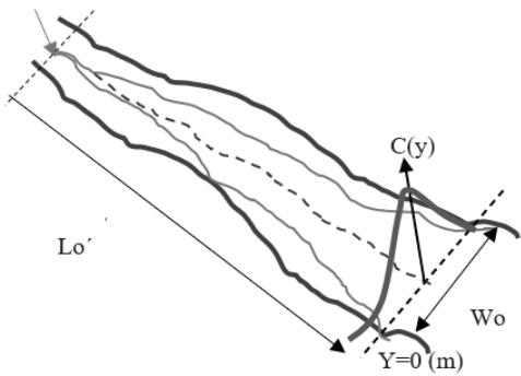Source:Author Figure 4: Curve C(y) in Wo, at distance Lo The Gaussian expression in terms of the transverse spatial variance for this case is, with Cp equal in C(X) and C(Y), since $t \approx 4\sqrt{2} * \sigma t$ for both distributions, as follows $$ \boldsymbol{C}(\boldsymbol{y}) \boldsymbol{i} \approx \boldsymbol{C}_{p} * e^{-\frac{(\boldsymbol{y} - \frac{\boldsymbol{W}}{2})^{2}}{2 * \sigma_{\boldsymbol{y}}^{2}}} \tag{21} $$ The function $C(t)$ in this case corresponds to the inflection points of the curve. $$ C(t)i \approx 0.608 * Cp $$ Therefore, eq. (21) would be put like this: $$ \frac {C p}{c 8) i} \approx e ^ {+ \frac {(y - \frac {W}{2}) ^ {2}}{2 * \sigma_ {y} ^ {2}}} \tag {23} $$ Rearranging: $$ \frac{1}{0.608} \approx 1.64 \approx e^{\frac{(y-\frac{W}{2})^2}{2*\sigma_y^2}} \tag{24} $$ And then, with $y = 0$: $$ Ln|1.64| \approx 0.50 \approx \frac{(W/2)^{2}}{2*\sigma_{y}^{2}} \approx \frac{W^{2}}{8*\sigma_{y}^{2}} \tag{25} $$ And then: $$ \sigma_ {y} \approx \frac {W}{2} \tag {26} $$ Then, concurrently with eq. (3), the tracer plume, when $\Phi \approx 0.38$, transversely occupies half of the plume width. Figure 5.  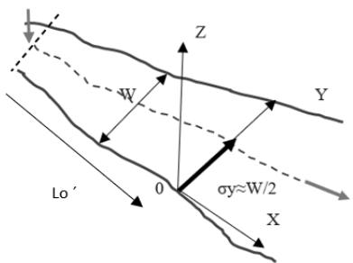Figure 5: Occupation of $\frac{1}{2}$ Flow Width by Diffusion transverse variance Therefore, dividing the two displacements, the longitudinal and the transversal, we have: $$ \frac{\sigma_x}{\sigma_y} \sim \frac{4\sqrt{2}}{1} \approx 4\sqrt{2} \tag{27} $$ ### c) Quantitative Description of this Dynamic to Find the Ratio of Centroid Time and Peak Time The author have already developed a successful approach for calculating the centroid-to-peak time ratio, " $t_s / t_p$," based on thermodynamic considerations, [27] as shown in Figure 5.  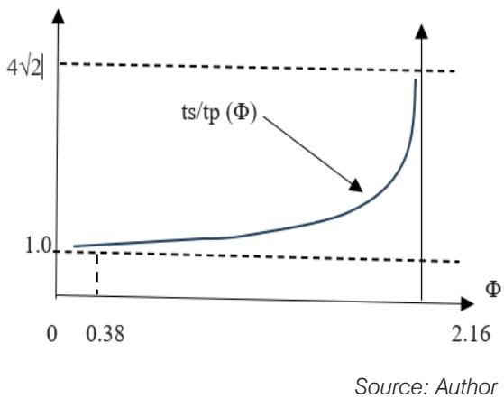Figure 5: Curve of the ts/tp ratio as a function of $\Phi(t)$ When $\Phi \approx 2.16$, the ts(tp ratio is maximum, close to $4\sqrt{2}$, which is the maximum allowed by the homogeneously distributed mass. For $\Phi < 0.38$, it asymptotically approaches 1.0, i.e., there is no delay in the solute centroid when electrostatic interactions between its particles cease. The approximate equation for this trend is: $$ \frac{ts}{tp} \approx 0.85 * \Phi^{2.2} + 1 $$ A notable value of this calculation is when $\Phi \approx 0.38$, the moment at which the solute changes to the ideal gas condition, and the electrostatic "braking" effect is reduced to a minimum: $$ \frac {t s}{t p} \approx 0. 8 5 * 0. 3 8 ^ {2. 2} + 1 \approx 1. 1 0 \tag {29} $$ Which means that the centroid delay is $10\%$, that is, at the limit of the order of magnitude to not be considered. d) Quantitative Description of this Dynamic to Find the Ratio of the Transport Coefficients $\Sigma_{x}$ and $\Sigma_{y}$. Now, based on results described in 4.2, it is interesting to find the relationship $\sigma_{x} / \sigma_{y}$, which corresponding curve is as shown in Figure 6.  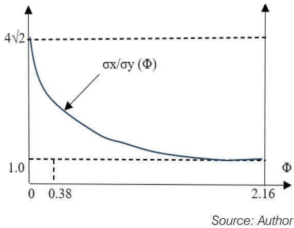Figure 6: Curve of the $\sigma_{\mathrm{x}} / \sigma_{\mathrm{y}}$ ratio as a function of $\Phi(t)$ A more detailed representation, including notable modeling points, is shown in Figure 7. 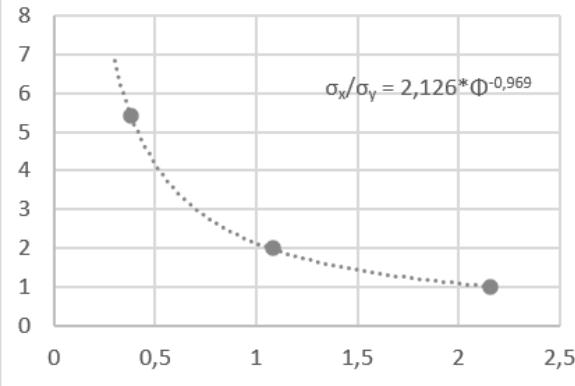$$ \sigma_{x}/\sigma_{y} (\Phi) $$  Source: Author Figure 7: Detailed Curve of the ratio $\sigma x / \sigma y$ as a function of $\Phi(t)$ The approximate equation for this trend is: $$ \frac {\sigma_ {x}}{\sigma_ {y}} \approx \frac {2 . 1 2 6}{\Phi^ {0 . 9 6 9}} \tag {30} $$ The notable points here are: For $\Phi \approx 2.16$, at the beginning of the process, the two variances are practically equal, and $\sigma x / \sigma y \approx 1$, given that the bias imposed by the advection shear effect is just beginning. For later events, when $\Phi \approx 0.38$, the two values progressively diverges to infinity. For this reason, as a practical limit of the expansion of the function, it is taken no longer to 0.38. Note that this limit is the one of interest, since up to this point, the "Mixing Length" is obtained. Therefore, the Gaussian ratio of the longitudinal and transverse transport coefficients will be: $$ \frac{\sigma_x}{\sigma_y} \approx \sqrt{\frac{E}{\varepsilon y}} \tag{31} $$ And therefore: $$ \frac{E}{\epsilon y} \approx \left(\frac{\sigma_{x}}{\sigma_{y}}\right)^{2} \tag{32} $$ Normally the longitudinal coefficient, E, is known, then the transverse coefficient will be: $$ \boldsymbol{\varepsilon} \mathbf{y} \approx \frac{E}{\left(\frac{\sigma_{x}}{\sigma_{y}}\right)^{2}} \tag{33} $$ This value of $\varepsilon y$ must be contrasted with the one calculated from the Elder corrected eq. (19), which is considered an acceptable standard for the channel under study. ## V. PRACTICAL APPLICATION OF THE METHOD TO REAL CHANNELS IN COLOMBIA AND USA ### a) Upper Guavio River, Colombia in 2001 For this study, we consider saline tracer (NaCl) experiments conducted by the Universidad de los Andes in Bogotá in 2001 on the upper Guavio River, a mountain, very roughness river near the town of Arbelaez in the center of the country. [28] Figure 8.  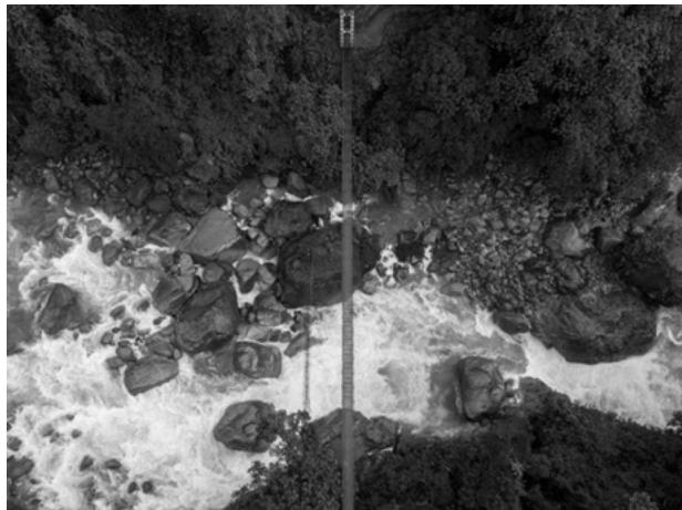Source: Author Figure 8: View of Rio Guavio, near Arbelaez. Colombia The data of this stream experiment is in Table 1. Table 1: Experimental data at Rio Guavio Source:Author <table><tr><td>Date: June 17, 2001. 2n station curve.</td></tr><tr><td>2ond curve length: X = 98.1 (m)</td></tr><tr><td>Width: W ≈ 10.0 (m)</td></tr><tr><td>Depth: H ≈ 0.25 (m)</td></tr><tr><td>Hydraulic radius: R≈0.22 (m)</td></tr><tr><td>Slope: S ≈ 0.045</td></tr><tr><td>Cross-sectional area: Ayz ≈ 2.3 (m2)</td></tr><tr><td>Roughness (Manning): n ≈ 0.32</td></tr><tr><td>Flow rate: Q ≈ 0.550 (m3/s)</td></tr><tr><td>Average velocity: U ≈ 0.24 (m/s)</td></tr><tr><td>Mass (NaCl): M ≈ 12233.0 (g)</td></tr><tr><td>Peak time: tp ≈ 410.0 (s)</td></tr><tr><td>State function: Φ ≈ 0.55</td></tr><tr><td>Longitudinal coefficient: E ≈ 0.77 (m2/s).</td></tr></table> 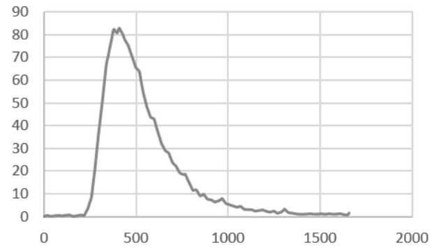The experimental tracer curve and its model, using equation (9), for that experiment at the second station, are shown in Figure 9.  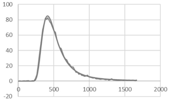C(t) E2, Guavio C(t) E2 Guavio Model,  Figure 9: Experimental curve (broken) and superimposed model (soft), using equation (10) Source: Author As can be seen at a distance of $\mathrm{X}1 = 98.1$ (m) and with a State Function of $\Phi 1 \approx 0.55$, does not yet reach the condition of complete mixing, which occurs at $\Phi \approx 0.38$, then the unknown distance, Lo, must be estimated approximately with the eq. (7): $$ \frac {\Phi 1}{\Phi 2} \approx \frac {\sqrt {X 2}}{\sqrt {X 1}} \tag {34} $$ Then: $$ \sqrt {X 2} \approx \sqrt {9 8 . 1} * \left(\frac {0 . 5 5}{0 . 3 8}\right) \approx 1 4. 3 3 \tag {35} $$ So: $$ X 2 \approx L o ^ {\prime} \approx 2 0 6. 3 (m) \tag {36} $$ Now, ratio $\sigma_{\mathrm{x}} / \sigma_{\mathrm{y}}$ eq. (30) is then calculated for $\Phi \approx 0.38$ $$ \frac {\sigma_ {x}}{\sigma_ {y}} \approx \frac {2 . 1 2 6}{(0 . 3 8) ^ {0 . 9 6 9}} \approx 5. 4 3 \tag {37} $$ And the transverse transport coefficient, $\varepsilon y$, is as in eq. (33): $$ \varepsilon y \approx \frac{E}{\left(\frac{\sigma_{x}}{\sigma_{y}}\right)^{2}} \approx \frac{0.77}{5.43^{2}} \approx \frac{0.77}{29.5} \approx 0.026 \left(\frac{m^2}{s}\right) \tag{38} $$ This Coefficient is verified against the value obtained by Elder: $$ \varepsilon y \approx 0. 6 * 0. 2 5 * \sqrt {0 . 2 5 * 9 . 8 3 * 0 . 0 4 5} \approx 0. 0 5 0 \left(\frac {m ^ {2}}{s}\right) \tag {39} $$ The ratio of the two results are 1.92, then, of the same order of magnitude, and are accepted as valid verification. The mixing length Lo, eq. (2), is then: $$ L _ {o} \approx \frac{0 . 1 * 0 . 24 * 10 ^ {2}}{0 . 026} \approx 92.3 (m) \tag{40} $$ Comparing with $\text{Lo}'$ calculated with eq. (7), it is noted that $\text{Lo}' > \text{Lo}$ and it is accepted that With a central injection ( $k = 0.1$ ) the dispersion covers the width of the channel, but as $\text{Lo}'$ is greater, the solute does not yet have a homogeneous distribution in its volume. Although the transverse diffusion coefficient has been calculated with a good approximation to the reference (Elder-Fischer), since there is no strict control over the exact injection, the multiplier "k" may vary. In this case, the $\text{Lo}'$ figure can be considered more precise since it does not depend on this factor. ### b) Rio Bogota, Colombia in 2024 The Bogota River near the flower farms in the capital is a small to medium-sized plain river with a gentle gradient. In this day were used fluorescent tracer (RWT). Figure 10.  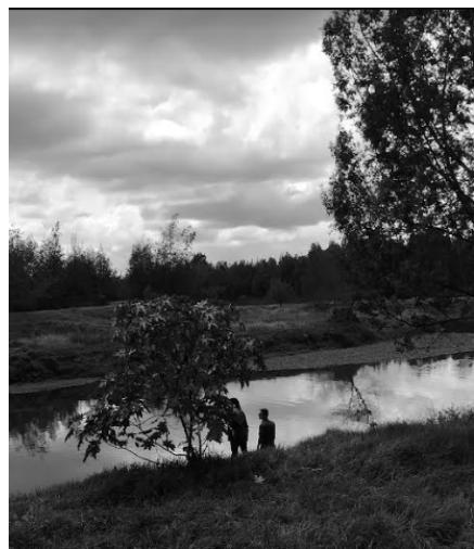Source: Author Figure 10: Bogota River, near capital, in Colombia. The river experimental data on that day were in Table 2. Table 2: Experimental data at Rio Bogota <table><tr><td>Date: September 5, 2024. 2ond station curve 2ond curve length: X = 3515.0 (m) Width: W ≈ 20.0 (m) Depth: H ≈ 2.3 (m) Hydraulic radius: R≈1.58 (m) Slope: S ≈ 0.0006 Cross-sectional area: Ayz ≈ 38.8 (m2) Roughness (Manning): n ≈ 0.025 Flow rate: Q ≈ 26.8 (m3/s) Average velocity: U ≈ 0.69 (m/s) Mass (RWT): M ≈ 160.0 (g) Peak time Second curve: tp ≈ 5097.0 (s) State function: Φ ≈ 0.167 Longitudinal coefficient: E ≈ 7.25 (m2/s).</td></tr></table> The experimental tracer curve and its model, eq. (10), for that experiment at the second station, are shown in Figure 11.  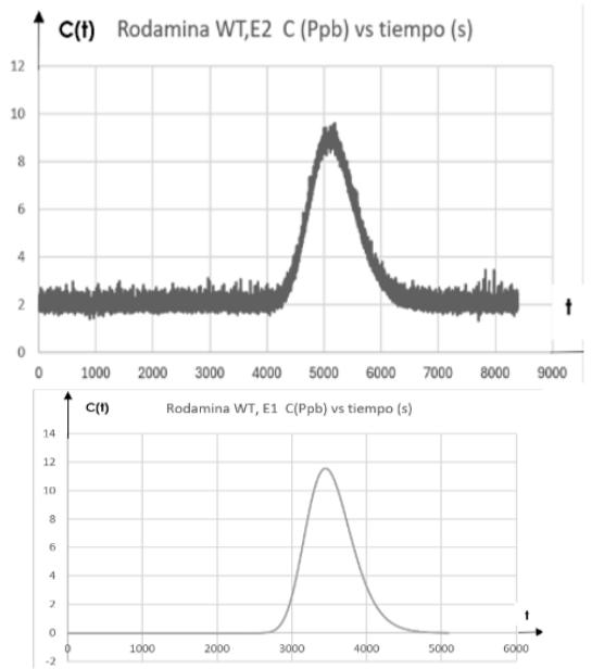Source:Author Figure 11: Experimental curve (red) and superimposed model (gray) As can be seen, the "Complete Mixing" condition for Dispersion was reached at an earlier point, since $\Phi < 0.38$, therefore equation (7) must be applied to calculate approximately the distance X1 at which it occurred with $\Phi_1 \approx 0.38$: $$ \sqrt {X 1} \approx \left(\frac {\Phi 2}{\Phi 1}\right) * \sqrt {X 2} \tag {41} $$ And then: $$ \sqrt {X 1} \approx \left(\frac {0 . 1 6 7}{0 . 3 8}\right) * \sqrt {3 5 1 5} \approx 2 6. 1 \left(m ^ {\frac {1}{2}}\right) \tag {42} $$ And therefore, $\mathrm{X}1 \approx \mathrm{Lo}^{\prime} \approx 681.0$ (m) Now, eq. (30) is then calculated for $\Phi \approx 0.38$: $$ \frac {\sigma_ {x}}{\sigma_ {y}} \approx \frac {2 . 1 2 6}{(0 . 3 8) ^ {0 . 9 6 9}} \approx 5. 4 3 \tag {43} $$ And the transverse transport coefficient, $\varepsilon y$, is in eq. (33): $$ \varepsilon y \approx \frac {E}{\left(\frac {\sigma_ {x}}{\sigma_ {y}}\right) ^ {2}} \approx \frac {7 . 2 6}{5 . 4 3 ^ {2}} \approx \frac {7 . 2 6}{2 9 . 5} \approx 0. 2 5 \left(\frac {m 2}{s}\right) \tag {44} $$ It is verified against the value obtained by Elder-Fischer: $$ \varepsilon y \approx 0. 6 * 2. 3 * \sqrt {2 . 3 * 9 . 8 3 * 0 . 0 0 0 6} \approx 0. 1 6 0 \left(\frac {m ^ {2}}{s}\right) (4 5) $$ The ratio of the two results are 1.56, then, of the same order of magnitude, and are accepted as valid verification. $$ L_{o} \approx \frac{0.1*0.69*20^{2}}{0.25} \approx 662.4\(m) \tag{46} $$ Comparing with $\mathrm{Lo}^{\prime}$, calculated with equation (7), it is noted that $\mathrm{Lo}^{\prime} \approx \mathrm{Lo}$ (same order) and it is accepted that the calculation on the width of the channel is equivalent to the criterion of homogeneous distribution of the tracer on the solute current tube. ### c) Caltech Channel, USA in 1966 A third example is documented, a tracer experiment carried out by H. B. Fischer [29] on the 40 (m) calibrated channel of the W. M. Keck Laboratory at Caltech, in 1966. In this experiment (Series 2700), Fischer injected NaCl as a tracer, measuring two sequential curves. The objective of the experiment was to test Elder's diffusion theory. Figure 12.  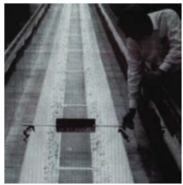Source: [3] Figure 12: W.M. Keck 40 (m) channel in Caltech. USA The channel experimental data on that day were in Table 3: Table 3: Experimental data at Caltech channel <table><tr><td>Date: 1966. 2ond station curve.</td></tr><tr><td>2nd curve length: X = 25.06 (m)</td></tr><tr><td>Width: W ≈ 1.09 (m)</td></tr><tr><td>Depth: H ≈ 0.128 (m)</td></tr><tr><td>Hydraulic radius: R≈0.104 (m)</td></tr><tr><td>Slope: S ≈ 0.0002</td></tr><tr><td>Cross-sectional area: Ayz ≈ 0.14 (m2)</td></tr><tr><td>Roughness (Manning): n ≈ 0.009</td></tr><tr><td>Flow rate: Q ≈ 0.053 (m3/s)</td></tr><tr><td>Average velocity: U ≈ 0.372 (m/s)</td></tr><tr><td>Mass (NaCl): M ≈ 40.5 (g)</td></tr><tr><td>Peak time 2ond curve: tp ≈ 67.4 (s)</td></tr><tr><td>State function 2ond curve: Φ ≈ 0.130</td></tr><tr><td>Longitudinal coefficient: E ≈ 0.0169 (m2/s).</td></tr></table> The experimental (dotted lines) two tracer curves and the models (thick continuous lines), are shown in Figure 13.  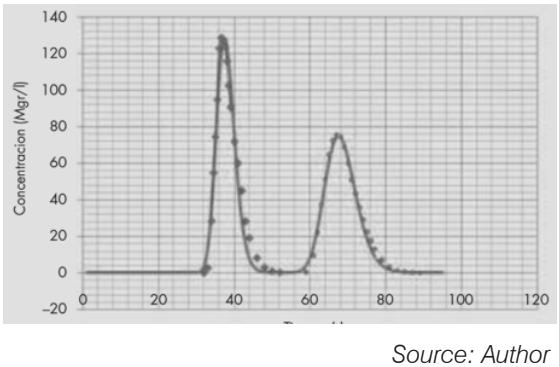Figure 13: Experimental curves (dotted) and superimposed model (thick continuous line) As can be seen, the "Complete Mixing" condition for Dispersion was reached at an earlier point, since $\Phi < 0.38$, therefore eq. (7) must be applied to calculate approximately the distance at which it occurred, with $X2 \approx 25.06 \, (\mathrm{m})$, and $\Phi 2 \approx 0.130$. It is necessary that $\Phi 1 \approx 0.38$ as explained. $$ \sqrt {X 1} \approx \left(\frac {\Phi 2}{\phi 1}\right) * \sqrt {X 2} \tag {47} $$ And then: $$ \sqrt{X1} \approx \left(\frac{0.130}{0.38}\right) * \sqrt{25.06} \approx 1.71 \left(m^{\frac{1}{2}}\right) \tag{48} $$ And therefore, $\mathrm{X}1 \approx \mathrm{Lo}^{\prime} \approx 2.93$ (m) Now, eq. (30) is then calculated for $\Phi \approx 0.38$ $$ \frac {\sigma_ {x}}{\sigma_ {y}} \approx \frac {2 . 1 2 6}{(0 . 3 8) ^ {0 . 9 6 9}} \approx 5. 4 3 \tag {49} $$ And the transverse transport coefficient, $\varepsilon y$, is in eq. (33): $$ \varepsilon y \approx \frac{E}{\left(\frac{\sigma_{x}}{\sigma_{y}}\right)^{2}} \approx \frac{0.0169}{5.43^{2}} \approx \frac{0.0169}{29.5} \approx 0.0006 \left(\frac{m^2}{s}\right) \tag{50} $$ It is verified against the value obtained by Elder: $$ \varepsilon y \approx 0.6 * 0.128 * \sqrt{0.128 * 9.83 * 0.0002} \approx 0.00122 \left(\frac{m^2}{s}\right) \tag{51} $$ The ratio of the two results are 4.92, not so convergent to unit, but of the same order of magnitude, and are accepted as valid verification. The mixing length Lo, eq. (2), is: $$ Lo \approx \frac{0.1*0.372*1.09^{2}}{0.0006} \approx 73.7\(m) \tag{52} $$ The two notable distances, Lo and Lo', differ greatly in their values, indicating that longitudinal dispersion achieves the mixing effect first, rather than transverse diffusion, which has an exaggeratedly high value for the special scope of the channel, indicating that probably in artificial channels, with very small Longitudinal transport coefficient, the indicated method to establish "Complete Mix" is the Lo' calculation. ## VI. RESULTS AND DISCUSSIONS 1. This article develops criteria to estimate when a flow reaches the "Complete Mixing" condition. When using the classic Rutherford formula, the transverse diffusion coefficient is calculated from the ratio of longitudinal and transverse variances, using a nonlinear distribution function of $\Phi$, and the value of the longitudinal dispersion coefficient. The values of these calculations are convergent with those found by the Elder-Fischer formula. The alternative criterion is based on finding the distance from the tracer at which $\Phi \approx 0.38$, and the solute is considered homogeneously distributed in the volume covered by the tracer. 2. The first criterion estimates that the tracer fills the channel width, while the second does not. 3. In real streams, the two criteria can sometimes converge, and sometimes not. In very large rivers (with very large widths), where the "mixing lengths" calculated using the classic formula are very long, the other criterion should be preferred, since the interest is often to determine the advection-dispersion characteristics at a certain intermediate point (not across the entire width). 4. To characterize the evolution of the conservative solute in the flow, a state function $\Phi$, is documented, which describes the different notable moments analyzed here. 5. To verify whether this value of $\varepsilon y$ is consistent with Elder's classic calculation, taken as a reference, the method is applied to a real field experiment. ### 1. Ministerio del Ambiente. Guia Nacional de Modelacion del recurso hídrico para agua - superficiales continentales. Bogota: Minambiente. 2018. 2. Elder J. W. The dispersal of marked fluid in turbulent shear flow. Journal of Fluid Mechanics, vol. 5, pp 544-560. 1959. 3. Fischer H. B. Longitudinal dispersion in laboratory and natural streams. PhD. Dissertation. Report No. KH-R-12, USA. June. 1966 4. Martin J. L. & McCutcheon S. Hydrodynamics and transport for water quality modeling. Boca Raton: Lewis Publishers, 1999. 5. French. R Open channel hydraulics. NewYork: McGraw-Hill, 1985. 6. Frish S. & Timoreva A. Curoso de Fisica general, Vol 1. Moscú: Editorial Mir, 1969. 7. Martin J. L. & McCutcheon S. Hydrodynamics and transport for water quality modeling. Boca Raton: Lewis Publishers, 1999. 8. Seo I. W. & Baek K. Estimation of longitudinal dispersion coefficient for streams. River Flow. Bousmar & Zech. Lisse, 2002. pp 143-150. 9. Martin J. L. & McCutcheon S. Hydrodynamics and transport for water quality modeling. Boca Raton: Lewis Publishers, 1999. 10. Holley, E. R. Unified view of diffusion and dispersion. J. Hydr. Div., ASCE, 95(2), pp 621-631. 1969. 11. Fischer H. B. Longitudinal dispersion in laboratory and natural streams. PhD. Dissertation, Report No. KH-R-12 California Institute of Technology, Pasadena. 1966 12. Damaskin B. & Petri O. Elementos de la electroquimica teorica. Moscu: Editorial Mir, 1981. 13. Elsgolltz L. Ecuaciones diferenciales y calculo variacional. Moscú: Editorial Mir, 1969. 14. Constain A. & Lemos R. Una ecuación de la velocidad media del flujo en régimen no uniforme, su relacion con el fenómeno de dispersion como funciona del tiempo y su aplicación a los estudios de calidad de agua. Revista ingeniería Civil No. 164. Madrid, pp 114-135. 2011. 15. Constrain A. The Svedberg Number, 1.54, as the Basis of a State Function Describing the Evolution of Turbulence and Dispersion. Exergy: Theoretical background and case studies. London: Intechopen book, 2024. 16. Vennard J. Elementos de la mecanica de fluidos. México: CECSA. 1965. 17. Guerasimov Ya. & Dreving V. & Eriomin A. & Kiseliov A. & Levedeb V. & Panchenkov G. y Shliguin A. Cuorso de Quimica fisica. Tomo 1, Moscu: Editorial Mir, 1980. 18. Damaskin B. & Petri O. Elementos de la electroquimica teorica. Moscu: Editorial Mir, 1981. 19. Guerasimov Ya. & Dreving V. & Eriomin A. & Kiseliov A. & Levedeb V.& Panchenkov G. y Shliguin A. - Curso de Química física. Tomo 1, Moscu: Editorial Mir, 1980. 20. Constín A. Definición y análisis de una función de evolución de solutos dispersivos en flujos naturales. Revista Dyna No. 175, pp. 173-181. 2012. 21. Bronstein I. & Semendiaev. Manual de Matemáticas. Moscú: Editorial Mir, 1973. 22. Frish S. & Timoreva A. Curo de Fisica general. Volume 1, Moscu: Editorial Mir, 1969. 23. Nekrasov B. Hidraulica. Moscu: Editorial Mir. 1965. 24. Baek K. & Seo H.W. Empirical equation for transverse dispersion coefficient based on theoretical background in rivers bends. Environ Fluid Mech (2013) 13: pp 465-477. 2013. 25. Baek K. O. & Lee D.Y. Development of simple formula for transverse dispersion coefficient in meandering rivers. Water 15(17):3120. pp 1-12. 2023. 26. Nekrasov B. Hidráulica. Moscú: Editorial Mir. 1965. 27. Constain A. & Lemos R. Una ecuación de la velocidad media del flujo en régimen no uniforme, su relacion con el fenómeno de dispersion como funciona del tiempo y su aplicación a los estudios de calidad de agua. Revista ingeniería Civil No. 164. Madrid, pp 114-135. 2011 28. Torres O. M. Investigación de la aplicación del modelo ADZ de transporte de solutos en un rio de montaña (Rio Guavio, M. Sc. Thesis, Universidad de los Andes. Bogotá, 2004. 29. Fischer H. B. Longitudinal dispersion in laboratory and natural streams. PhD. Dissertation, Report No. KH-R-12 California Institute of Technology, Pasadena. 1966

Generating HTML Viewer...